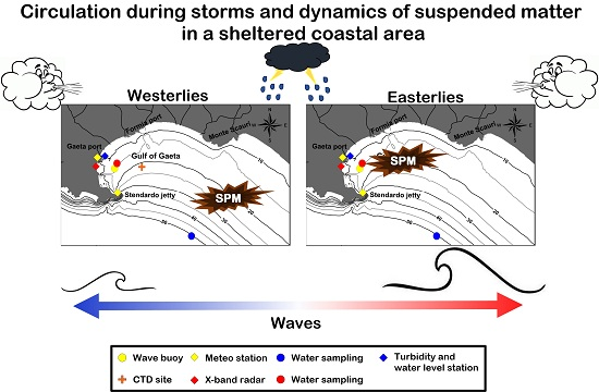
Circulation during Storms and Dynamics of Suspended Matter in a Sheltered Coastal Area

Abstract

The Gulf of Gaeta, in the western margin of central Italy, is characterized by a coastal morphology that creates a natural sheltered area in which fine sediment settles. The new port regulatory plan provides for dock expansions and dredging works that could alter the suspended particulate matter (SPM) concentration. The present study investigates the dynamics of the Gulf of Gaeta with a focus on the dynamic processes that affect the fine particle concentration. The study was conducted through a multidisciplinary approach that involves remote sensing acquisitions (satellite imagery and X-band radar), measurements in situ (water sampling, wave buoy, weather station, turbidity station, CTD profiles), and numerical modelling (SWAN and Delft3D FLOW). The X-band radar system supports the analysis of the dynamic processes of the SPM concentration providing a large dataset useful for the hydrodynamic model’s validation. The analysis reveals a strong influence of nearby rivers in modulating the SPM at the regional scale. Short-term high and low fluctuations in SPM concentration within the gulf are triggered by the local effect of the main physical forces. In particular, the direction of events and bottom sediment resuspension play a key role in modulating the SPM concentration while micro-tidal regime does not appear to influence turbidity in the study area. This approach represents an important tool in improving the long-term coastal management strategy from the perspective of sustainable human activities in marine coastal ecosystems.

1. Introduction

Estuaries and coasts are precious and sensitive environments that have remained strategic points of human settlement through history, with consequent persistent and intense impacts on coastal ecosystems [1]. Marine and terrestrial processes constantly affect coastal areas and influence their evolution over various time scales. Flows and sediments input on a continental shelf depend largely on the climate of a region and on the characteristics of the local catchment area, which together influence the hydrology of rivers [2,3]. The terrestrial inputs of material and the interactions between continental waters and coastal dynamics drive deposition and transport processes that influence ecological conditions for species reproduction and development. In the Mediterranean Sea, the terrestrial inorganic inputs are major fertilization sources, especially in the Adriatic and Aegean Basin [4], and the continental inputs influence food webs and the maintenance of fishing stocks in estuarine and coastal seas [5,6]. Rapid land cover changes over wide areas into the watershed also impact water and sediment fluxes. This has caused a significant shift in ecosystem dynamics, and scientific evidence of the adverse effects of anthropogenic fluxes are demonstrated by, as an example, a continuous decline in seagrasses [7,8], which represents a biodiversity hotspot in the Mediterranean Sea [9].

The interactions between terrestrial inputs and circulation forcing was previously investigated in several coastal sites such as the South Atlantic Bight [10], Mobile Bay [11,12], the Columbia River Delta [13], the Patos Lagoon [14] and the Black Sea [15]. Numerous studies in Mediterranean coastal areas focused on the dynamic of SPM discharged by the Rhône [16,17] and Po rivers [18], which are the main rivers of the Mediterranean Basin. Some studies have assessed coastal areas influenced by smaller rivers [19,20] that, despite their low flows, can also have a high local impact because they rapidly bring terrestrial material to the sea. These studies are accomplished through field data analysis, remote sensing, and analytical and numerical model experiments. Studies conducted in the Mediterranean Sea primarily focus on the analysis of nutrients, organic matter and contaminants released; multidisciplinary approaches of the coastal processes that affect the distribution of suspended particulate matter are currently rare for the Italian coastal area.

Remote sensors have enabled synoptic studies that monitor oceanic and atmospheric phenomena, such as marine pollution [21], algal blooms [22] and river plume dynamics [14]; however, their application (in the case of satellite data acquired at visual or infrared spectral bands) is often limited to cloud-free days and, furthermore, to large-scale patterns due to their low spatial resolution [23,24]. The radar systems within remote sensors allow measurements of the sea state and surface currents with accuracy and spatial resolution. The ‘Remocean’ system provides a surface current estimation using a normalized scalar product procedure developed by Serafino et al. [25], which has given robust agreement with respect to in situ observations [26] and demonstrates an ability to resolve turbulent structures observed within the coastal boundary layer [27]. This work is the first to use an X-band radar system to analyze the hydrodynamic processes and the associated dynamics of suspended particulate matter.

Sediment flux toward the sea is primarily driven by natural factors (geography, geomorphology, geology, and climate change) [2] and large-scale human activities such as dams, jetties, and other coastal constructions. These factors challenge natural processes and alter the sedimentary balance [28].

Previous studies demonstrated that the river plume dynamic is primarily controlled by the wind intensity and direction [29,30,31,32] and tidal action [33,34,35]. Together with terrestrial inputs, the resuspension of bottom sediments modulates the turbidity of coastal waters. In shallow, micro-tidal environments, the resuspension is primarily induced by surface gravity waves; however, in a sheltered coastal area, wind stress plays a fundamental role in bottom sediment resuspension [36,37].

Marine phenomena, such as flooding and erosion during storm events, represent a natural source of damage to coastal systems [38] and human properties. In micro-tidal environments, such as the Mediterranean Sea, storm waves are the principal driver of short-term coastal erosion and flooding and are the main factor controlling the hydrodynamics that lead to the morphological structure of beaches. In the Mediterranean Sea, storms originate from the “sub-synoptic lows” triggered by the major North Atlantic synoptic systems entering the Mediterranean Sea [39]. The study area is located on the western margin of central Italy and focuses on a gulf with characteristic exposure to meteorological events. This morphological feature produces a naturally sheltered area that is characterized by the settling of fine sediments. Humans have long taken advantage of its natural morphology and have urbanized the surrounding land. There are many marine activities such as those associated with ports as well as fish and mussel farming. The new port regulatory plan provides for dock expansions and dredging works that could alter nearby suspended particulate matter (SPM) concentrations.

This study is the first to investigate the dynamic of the Gulf of Gaeta with a focus on the dynamic processes that affect fine particle concentration within a coastal site. In the analyzed coastal area, the presence of a river delta is a natural source of siltation that stresses benthic communities [40], and new coastal works may further enhance the pressure on benthic organisms.

The study was conducted in a multidisciplinary approach that involves remote sensing acquisitions (satellite imagery and X-band radar), in situ measurements (water sampling, wave buoy, weather stations and turbidity stations) and numerical modelling (SWAN and Delft-3D FLOW). Knowledge regarding the natural fluctuations in turbidity in the study area represents an important tool for recognizing the effects of human activities on marine environments. This enables a more effective coastal management strategy that is based on suitable threshold values during dredging activities.

2. Materials and Methods

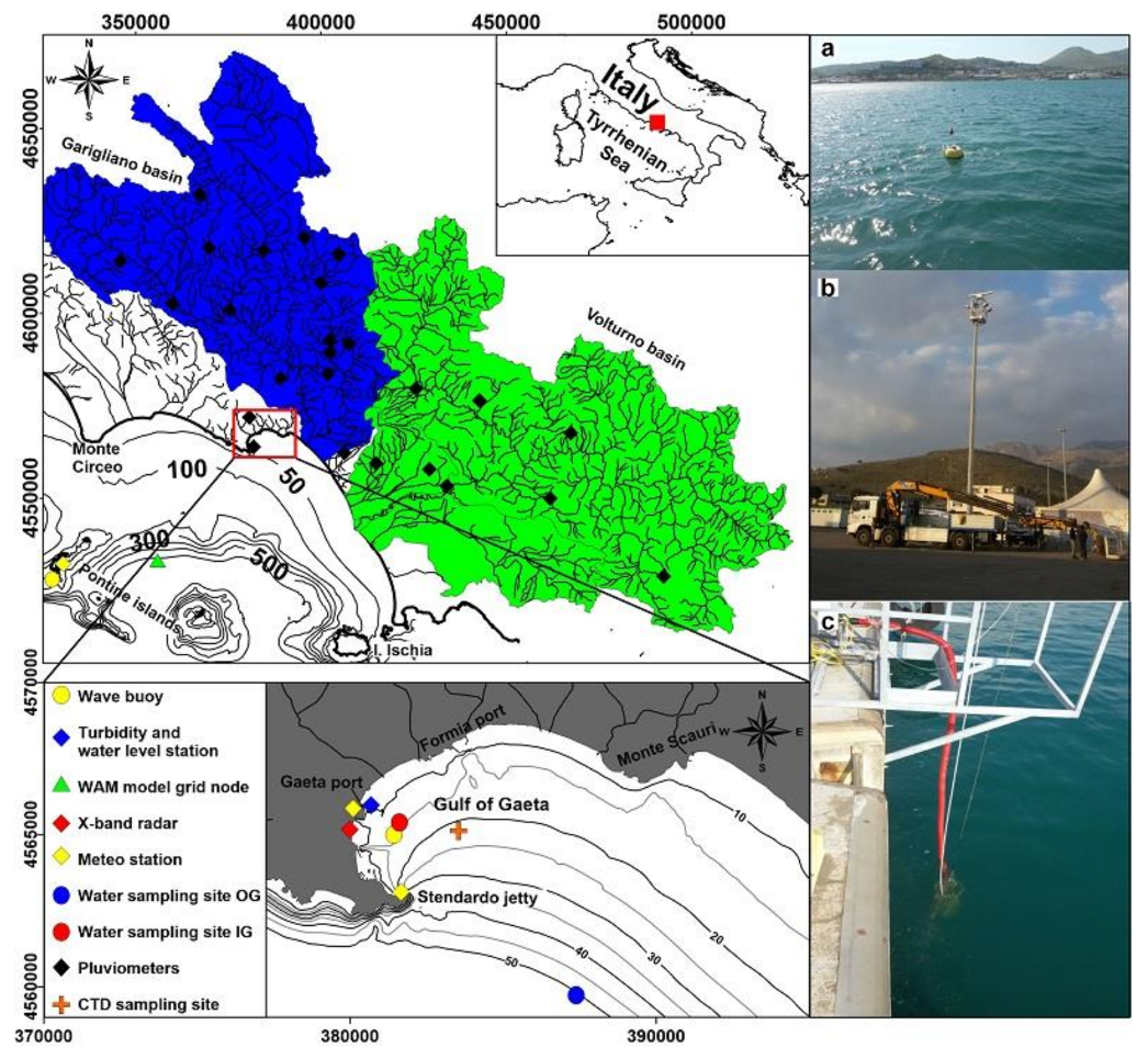
2.1. Morphological and Sedimentologic Aspects of the Study Area

The study area is enclosed within the coastal stretch between Mt. Circeo (North) and Mt. Procida (South) in the Central-Eastern Tyrrhenian Sea, Italy, which includes the southern part of the Lazio region and the northern part of the Campania region (Figure 1). The coastal area overlooks the archipelago of the Pontine Islands, which extends for more than 30 km parallel to the mainland coast.

The mainland morphology is affected by the Aurunci Mountains with high rocky shorelines in the north sector and by the alluvional deposits of the Garigliano and Volturno rivers in the southern sector [41] (Figure 1). The high rocky shorelines are primarily composed of carbonates, and arenaceous formations occur proceeding south from the Garigliano River [40]. The coastline morphology of the Gulf of Gaeta, which separates the southern and northern sectors of the study area, is completely transformed in armor coast, where multiple anthropic activities such as naval traffic and fisheries persist. The continental shelf shows a maximum extension in the southern sector near the Garigliano river mouth (approximately 20 km). This shelf narrows proceeding southward and northward (approximately 10 km) [42]. The Garigliano River drains the territories between the Aurunci mountains and Mt. Massico, and its coastal plain is delimited northeast by the Roccamonfina volcano [43,44]. Among the southern Italian rivers, the Volturno River has the highest mean flow (approximately 102 m³ s⁻¹), and the mean flows of this river were higher than those of the Garigliano [45]. Fresh waters from the Garigliano River appear to have a limited influence on a coastal area that extends north from the river up to the Gulf of Gaeta, while the Volturno River waters are distributed both northward and southward [40]. The Garigliano river bed load sediments are primarily composed of calcite and dolomite, whereas the Volturno river bed load sediments have high quartz, feldspar and smectite contents. Comparable mineral associations were found in the suspended loads of the Garigliano and Volturno rivers and in the marine environment [40,41]. The sediment distribution of the study area appears to be strongly influenced by the Volturno and Garigliano rivers. The northern sector of the study area shows sediment distribution that is clearly influenced by fine materials from the Garigliano River. The influence of this river extends up to the Gulf of Gaeta, where sediments finer than those normally found at the same depths are present [40,46]. The mean grain-size within the Gulf shows values from 0 to 5 phi, corresponding to coarse sand and coarse silt respectively. Furthermore, the sediment texture is characterized by an eastward decreasing muddy component, from 63% near Stendardo jetty to 6% near Monte Scauri [47,48]. This gradient reflects the benthic biocenosis structure which varies from typical muddy bottoms biocenosis to those of mixed-sediment bottoms with a high detritus content [40].

2.2. Brief Description of Methodology

The aim of the study is to analyze the contribution of main physical forcings on the coastal dynamic of the Gulf of Gaeta using an integrated approach involving in situ measurements, remote sensing observations and numerical simulations. The proposed approach/methodology is based on the following steps:

-

An analysis of wave data to determine storm classes and the characteristics of storm waves (see paragraph 3.1);

-

The reproduction of surface currents and wave fields induced by storm events using numerical models and comparison with X-band radar measures (see paragraph 3.2);

-

An analysis of the pattern distribution of the suspended particle matter (SPM) concentration at the regional scale based on satellite imagery (see paragraph 3.4);

-

An evaluation of the contributions of the physical forcing on the coastal dynamic within the Gulf of Gaeta (see paragraph 3.5).

The instruments and techniques used in this work are reported in the following paragraphs.

Wave data records were used to define the characteristics of waves in the study area, and statistical analyses of storms were used to determine the storm classes and the characteristics of storm waves.

The circulations induced by the various storm classes were then reproduced by DELFT-3D numerical models to reproduce historical events in the study area. The ‘Remocean’ X-band radar system acquired current field and waves data for the reproduced events. A comparison of the surface current and wave data recorded from radar acquisitions and numerical model simulations enables the dynamic characterization of the gulf of Gaeta during storm conditions. The structure of the water column was analyzed during 2013–2017 within the gulf. The satellite imagery collected for 2013–2017 were analyzed to define distribution patterns at the regional scale of SPM. This was assessed together with the rains falling in the study area river basins as well as the patterns obtained via satellite imagery to indicate the regional variability in the SPM concentration. The satellite information regarding the SPM concentration is validated by monthly water samplings at a location outside the gulf (OG) at a 50-m depth more than 5 km from the coast (Figure 1). Simultaneous water sampling was also conducted inside the gulf (IG) at a 10-m depth (Figure 1) to compare the monthly trend of turbidity inside and outside the gulf along a 4-year timescale. In particular, the time series of turbidity recorded inside the gulf was analyzed to statistically define the high (H) and low (L) turbidity and to determine their relationship with the dynamic forcing of the coastal system (wind intensity and direction, intensity of waves, water level fluctuation and rain).

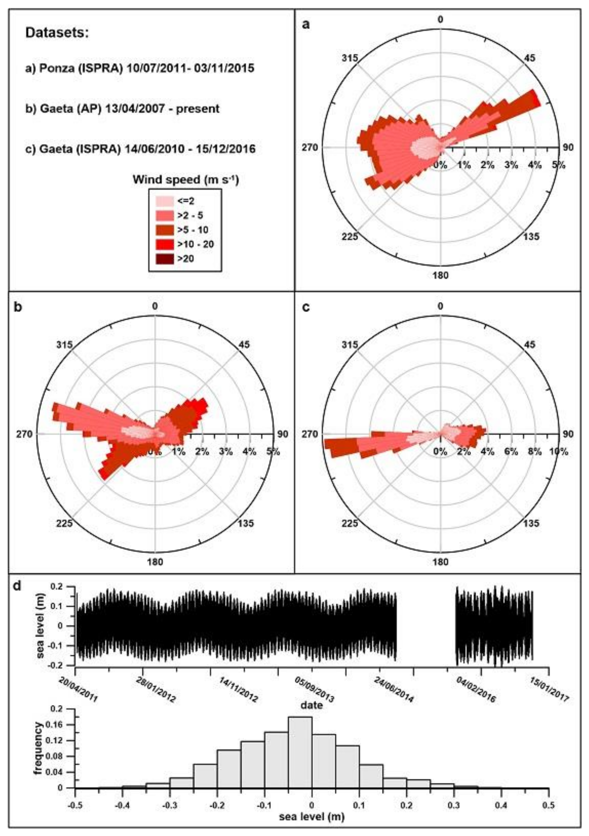
2.2.1. In Situ Data acquisitions

To describe the meteorological conditions of the study area, we considered the records of three weather stations, two located inside the Gulf of Gaeta, respectively, at Gaeta port and at Stendardo Jetty, and one placed at Ponza Island (Figure 1). The weather stations inside the port have been operating since 2007 and perform hourly recordings at 10 m above sea level for wind intensity and direction, rainfall, air temperature, relative humidity, atmospheric pressure, and solar radiation. The station at Punta Stendardo, which is the property of ISPRA, was in operation from 2010 to 2016 and performed hourly recordings of the intensity and direction of the wind, as well as atmospheric pressure, relative humidity, air temperature and sea level.

To analyze the storms in the study area, wave data were collected by wave buoys located both offshore and onshore at the study site (Figure 1). The wave buoy is a TRIAXIS directional wave buoy moored offshore at Ponza Island in correspondence of 100 m depth. The buoy recorded waves from 1989 to 2008 and was the property of RON-ISPRA (National Ondametric Network-Superior Institute of Environmental Protection). The offshore wave conditions used for model simulation, which dated to 2016 and 2017 when the Ponza buoy was missing, were retrieved from a deep water (approximately 600 m depth) grid point of the WAM Model of the Mediterranean Sea Waves Forecasting System of the Copernicus Marine Environment catalogue. The WAM model developed by HCMR, Greece and CMCC, Italy, provides statistical parameters of waves with a spatial resolution of 4 km and temporal resolution of 1 h.

The wave buoy placed nearshore was a ‘Datawell’ buoy deployed into the Gulf of Gaeta at a depth of 10 m that operated in 2013 and 2014.

To analyze the effect of the tidal excursion on the dynamics of the gulf, we calculated the tidal component originating from the total sea level record of the Italian Mareographic Network station. The marigraph station is installed on the quay of the Guardia di Finanza of Gaeta. The station is equipped with altimetric landmarks. Each benchmark refers to the mean sea level measured in Genoa by the ancient Thompson marigraph. The high precision altitude refers to the zero established by the IGM (Military Geographic Institute). Sea level records were analyzed via standard harmonic analysis with the T-Tide tool [49].

Given the lack of river discharge data of the Volturno and Garigliano rivers as well as small streams during the study period, we evaluated the run-off contribution to the turbidity of the Gulf of Gaeta with pluviometric measurements from 25 stations (Figure 1) located in the river basins of the study area. Because river basins fall into two different Italian regions, we collected data from the Hydrographic Service of the Latium Region (http://www.idrografico.roma.it/) and from the Centro Agrometeorologico of Campania (http://www.agricoltura.regione.campania.it/meteo/agrometeo).

To analyze the effect of the fresh water contribution within the Gulf the water column structure was studied at monthly interval between 2013 and 2017 at single point station within the Gulf of Gaeta at 25 m depth (Figure 1). All samplings were carried out from a small boat typically around 12:00 a.m., using a IDRONAUT-316 plus CTD probe. The sampling rate for the CTD was 10 Hz and was done allowing the probe to the freefall at an average descendent rate of 1 ms⁻¹. To measure the. The data were smoothed by kernel function and visualized in ODV software as T-S diagram. Salinity and density were calculated using EOS 80, UNESCO equation.

To test the optical SPM algorithm applied on satellite imagery and to compare the SPM concentration between the near-shore and off-shore zones, surface water samples were collected monthly at the two stations, IG and OG. These samples were then transported to the laboratory for specific analysis for suspended solid load. The determination was based on gravimetric filtration on a pre-combusted GF/C filter. The filter was then dried in an oven at 100 °C and weighted until the weight was constant (precision < 0.1 mg). The dried mass was then converted to SPM concentration by accounting for the volume of the filtered water (mg L⁻¹).

The measure of turbidity was performed by a Cyclops-7™ Submersible Sensor turbidimeter made by Turner Design (San Jose, CA, USA). The Turbidity Cyclops measures turbidity using an 850 nm light source and detects scattered light at a 90-degree angle. The sensor was installed on 27 October 2015 at a one-meter depth and was powered by a PV panel. The system collected data every 20 min and sent data via a Wi-Fi connection. The data on turbidity were statistically analyzed and placed in relation to the dynamic forcing of the coastal system. The data found the best fit with a Burr distribution , through which the mean, 5th and 95th percentile was calculated. These percentiles were chosen as a threshold to separate events with H and L turbidity. The H and L turbidity events were filtered from the time series and aligned with the dynamic factors. The distributions, associated with H and L events, of each dynamic variable were compared using the non-parametric Wilcoxon signed-rank test to determine the statistical dissimilarity of the two distributions; Pearson correlation analysis was also performed to assess the relationship between dynamic factors and turbidity.

2.2.2. Remote Sensing Observations

At the regional scale, the dynamic of SPM was studied through MODIS Aqua satellite imagery. This satellite assesses Earth’s surface every day and provides data available on the NASA EOS Data Gateway [50] in HDF format. Thanks to a specific processing tool, calibrated reflectance images can be obtained (http://oceancolor.gsfc.nasa.gov). Level 1A represents scans (MYD01) of counts of raw radiances and is ordered and downloaded from the NASA site via file transference protocol software. The SeaWiFS Data Analysis System (SEADAS, Version 6.4 available on seadas.gsfc.nasa.gov) was used to geolocate, apply atmospheric corrections and finally generate the calibrated radiances file using a chain-processing dataset (from an L1A level until an L2 product as an ascii map). Atmospheric correction was carried out using an L2 file generating program, where we applied an aerosol option mode, which was indicated as a “2-band model selection and MUMM NIR correction”, the modified algorithm that performs better in turbid waters [51]. The normalized water-leaving radiance of 645 (nLW 645, mW·cm⁻²·μm⁻¹·sr⁻¹) with a resolution of 250 m, corrected and selected, was our final product from the ‘Seadas’ elaboration to retrieve a geolocated distribution map of the sea surface area. The nLW645 spectral data were employed to estimate SPM through the optical algorithm developed for optically complex coastal waters by Ondrusek et al. [52] in the form of a 3rd order polynomial Equation (1):

TSM [mg L⁻¹] = 3.8813 (nLW(645))3 − 13.822 (nLW(645))2 + 19.61 (nLW(645))

(1)

At the local scale, an X-band radar system was installed in the Gulf of Gaeta (Figure 1b) in 2015 with the main aim of real-time monitoring of hydrodynamic conditions during storms and providing information regarding the sea state parameters in terms of sea surface currents and waves. Radar image analysis was performed by a ‘Remocean’ system, which has in recent years demonstrated the ability to provide a very robust determination of the currents field and sea state [27,53]. The physical possibility of extracting information on the sea surface from a radar signal is due to Bragg scattering. In particular, X-band electromagnetic waves are a few centimeters long and interact with the sea capillary waves, which ride on the gravity waves. The signal backscattered from the sea surface (clutter) is assessed by data processing procedures that are necessary to estimate the characteristic sea state parameters, such as wavelength, direction, period of the dominant wave and the significant wave height as well as surface current. The methodology of raw data processing is fully described in detail by several works [25,26,27,54], and in particular, the determination is performed by the “local method” based on the normalized scalar product, which has been proven to be the most accurate in obtaining the sea surface current and bathymetry fields from X-band radar images [25,27,54,55]. Once the radar is installed, it can operate continuously. However, measurements are significant only when the signal reflected from the Bragg resonance mechanism is high, indicating significant surface roughness. Due to the natural sheltering of the coastal site, events with sufficient intensity to produce radar records are not common, and February 2015 to September 2017 produced 20 storm events lasting from a few hours to some days. During these events, with meaningful presence of sea waves and local wind, to allow radar measurements, every image radar was carefully analyzed considering only the part in which the signal reflected by the mechanism of resonance of Bragg is important (with a sufficient surface roughness).

The radar system, installed in February 2015, is composed of a Marine Sperry X-band radar radiating a maximum power of 25 kW and equipped with a 9-foot (2.74 m) antenna. The radar antenna is located at the coordinates of Lat. 41.232612 N, Lon. 13.573088 E at the top of the lighting pole (15 m above sea level) in front of the sea within the port of Gaeta (Figure 1), and the details of the acquisition parameters are given in

Table 1. Setting of acquisition parameters.

Radar Parameter	Title 3
Peak power (kW)	25
Radar scale (NM)	2.48
Antenna rotation (sec)	1.94
Spatial image spacing (m)	4.4
Antenna height (m)	15
View angular sector (°N)	117

.

2.2.3. Numerical Simulations

To analyze water circulation patterns induced by storms within the Gulf of Gaeta, mathematical models included in the DELFT3D package were used. Specifically, DELFT3D-FLOW [56] was used to calculate currents, and SWAN [57] was used to simulate wave propagation toward the coast. The governing equations of these models are detailed in Lesser et al. [56] and Bonamano et al. [58]. The DELFT3D-FLOW and SWAN models use the same computational grid built within a rectangular domain that covers 60 km of the coastal area. Because small errors may occur near the boundaries, the study area was positioned away from the sides, approximately in the center of the model domain. The lateral boundaries are located near Terracina in the north and around the Volturno mouth in the south (see Figure 1). The offshore boundary is positioned at a mean distance of approximately 30 km from the coastline at a 100-m depth where deep water conditions can be assumed. The governing equations of DELFT3D-FLOW and SWAN were solved on a finite difference curvilinear grid with approximately 7000 elements. To limit computational requirements, a different resolution was applied in the model domain extending from 50 × 50 m in the Gulf of Gaeta to 1 × 1 km near the seaward boundary. The comparison between the model results with the sea state parameters (currents and waves) measured by the X-band radar system within the gulf of Gaeta was performed during storm events that occurred between 2015 and 2017.

In DELFT3D-FLOW, Neumann boundary conditions were applied on the lateral boundaries in combination with a water-level boundary on the seaward side, which is necessary to ensure that the solution of the mathematical boundary value problem is well posed. In the vertical direction, 10 sigma layers with higher resolution near the surface were considered to better reproduce the sea currents in the first layer of the water column and to ensure sufficient resolution in the near coastal zone. The hydrodynamical simulations lasted 72 h using a time step of 60 s. The day before the sampling period was used as a spin up time to reduce the noise that was introduced through the initial conditions. The wind drag coefficient was assumed to linearly depend on wind speed, varying from 0.00063 at 0 m/s to 0.00723 at 100 m/s. Because the sea bottom within the Gulf of Gaeta is primarily composed of mud sediments, the bed roughness is uniform in the space with a Chezy value equal to 60 m^1/2 s⁻¹ [59]. To solve the horizontal moment equations and to obtain the best correlation between the modeled results and measured data, horizontal background eddy viscosity and diffusivity were set to 1 m² s⁻¹ [60]. To account for the turbulence effects and to determine vertical viscosity and diffusivity, the K–e turbulence model was used [61].

In SWAN, the spectral action balance equation was resolved including the contributions of bottom friction, whitecapping and depth-induced breaking in wave energy dissipation terms. Specifically, bottom friction was parameterized using the JONSWAP formulation with a coefficient of 0.067 m² s⁻³, whitecapping was based on a pulse-based model [62] and depth-induced breaking was calculated using the Battjes and Janssen [63] model with a breaking parameter of 0.73. The hydrodynamic conditions of the study area are primarily controlled by wind and wave forcing because vertical variations of temperature and salinity within the Gulf of Gaeta are very small during the simulated periods. Tidal forcing has also been neglected because the maximum astronomical tide does not exceed 0.2 m during the simulation days according to the data recorded by the Italian Mareographic Network station. Given the proximity of the Gaeta Port weather station to the zone monitored by radar and the lack of another anemometer in the study area, DELFT3D-FLOW was fed with the wind speed and direction was measured by the Gaeta station. The wave effects were included in the DELFT3D-FLOW simulation by running a SWAN model every 30 min in on-line mode. Along the sea boundaries, the model was forced with the JONSWAP wave spectra [64] obtained from wave parameters calculated by a WAM model at the offshore site (Figure 1). The WAM model results are included in CMEMS (Copernicus Marine Environment Monitoring Service), which provide freely available hourly wave parameters at a 1/24° horizontal resolution covering the entire Mediterranean Sea.

DELFT3D-FLOW and SWAN results were compared with the magnitude of velocity components in the surface layer, the directional wave spectra and statistical parameters as measured by the radar system using the correlation coefficient (R) and Bias and Root Mean Square Error (RMSE), which provides a measure of the discrepancy between the predicted and measured data.

3. Results

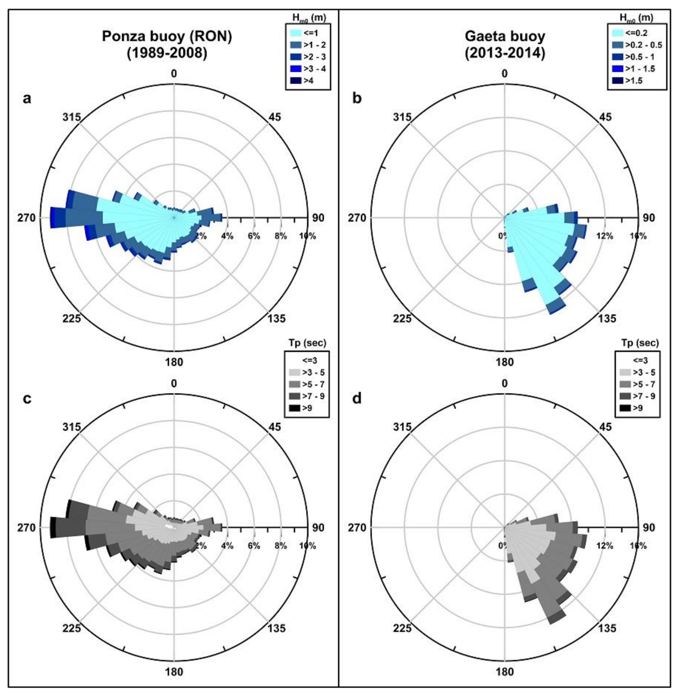
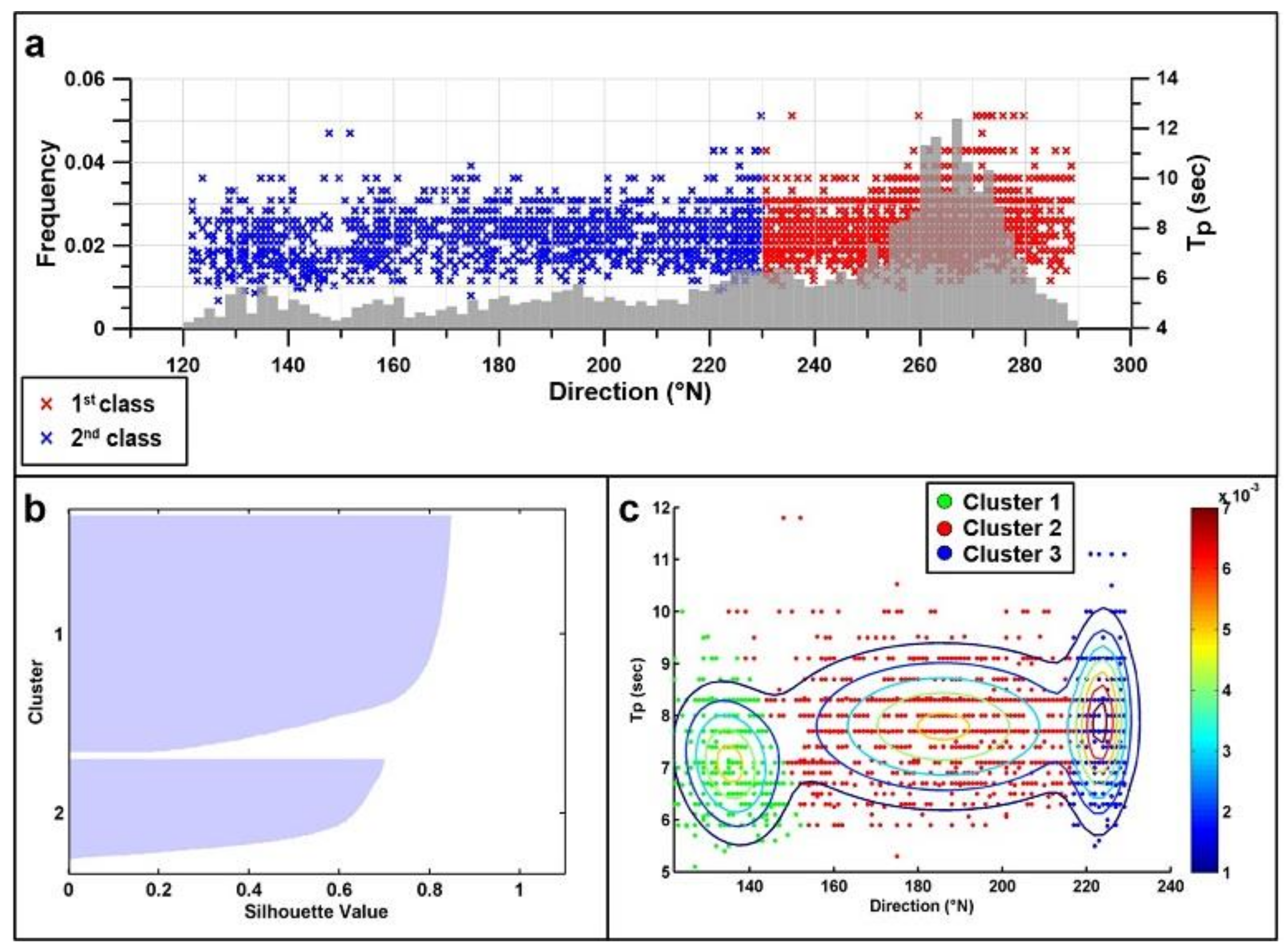
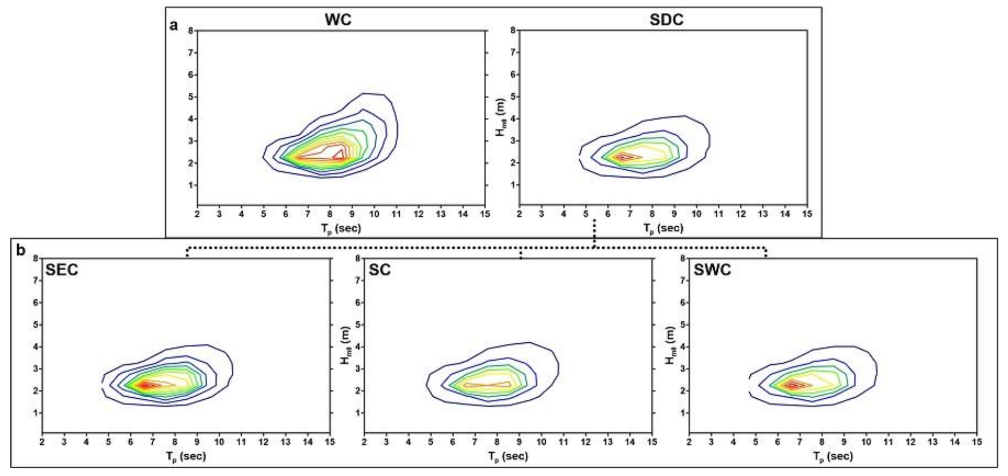
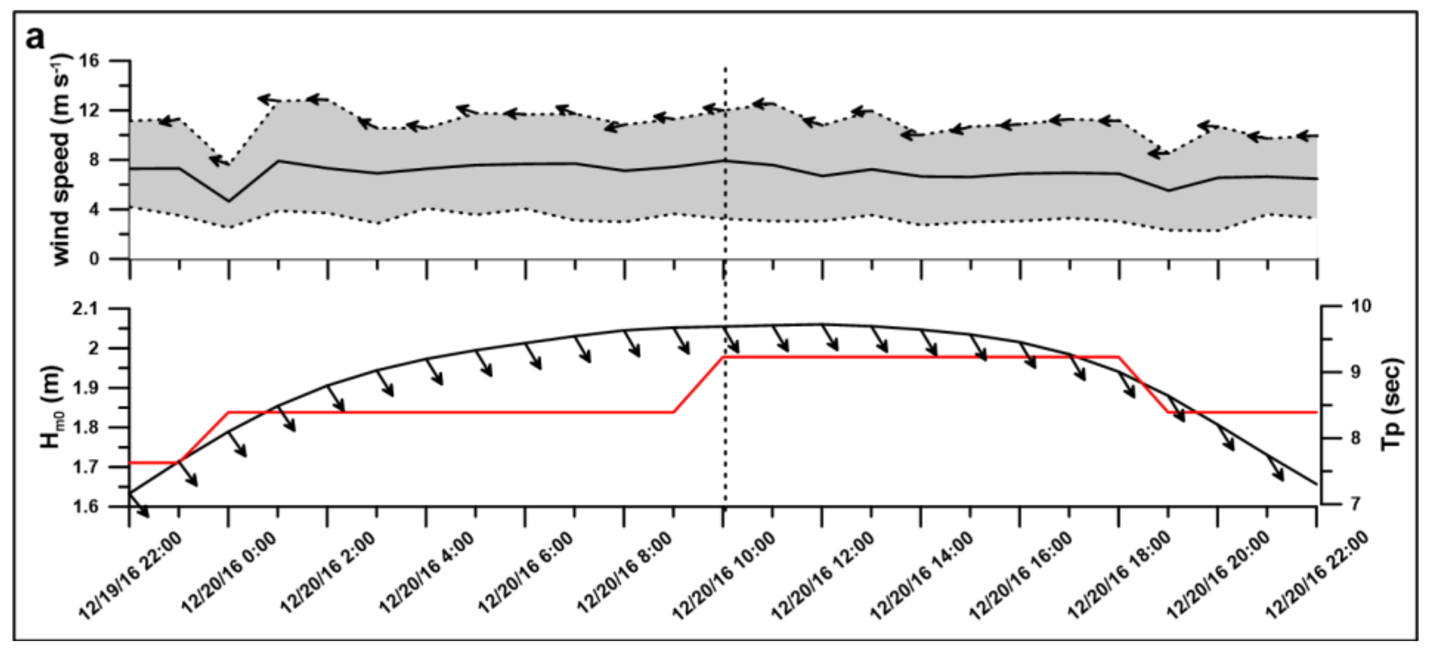
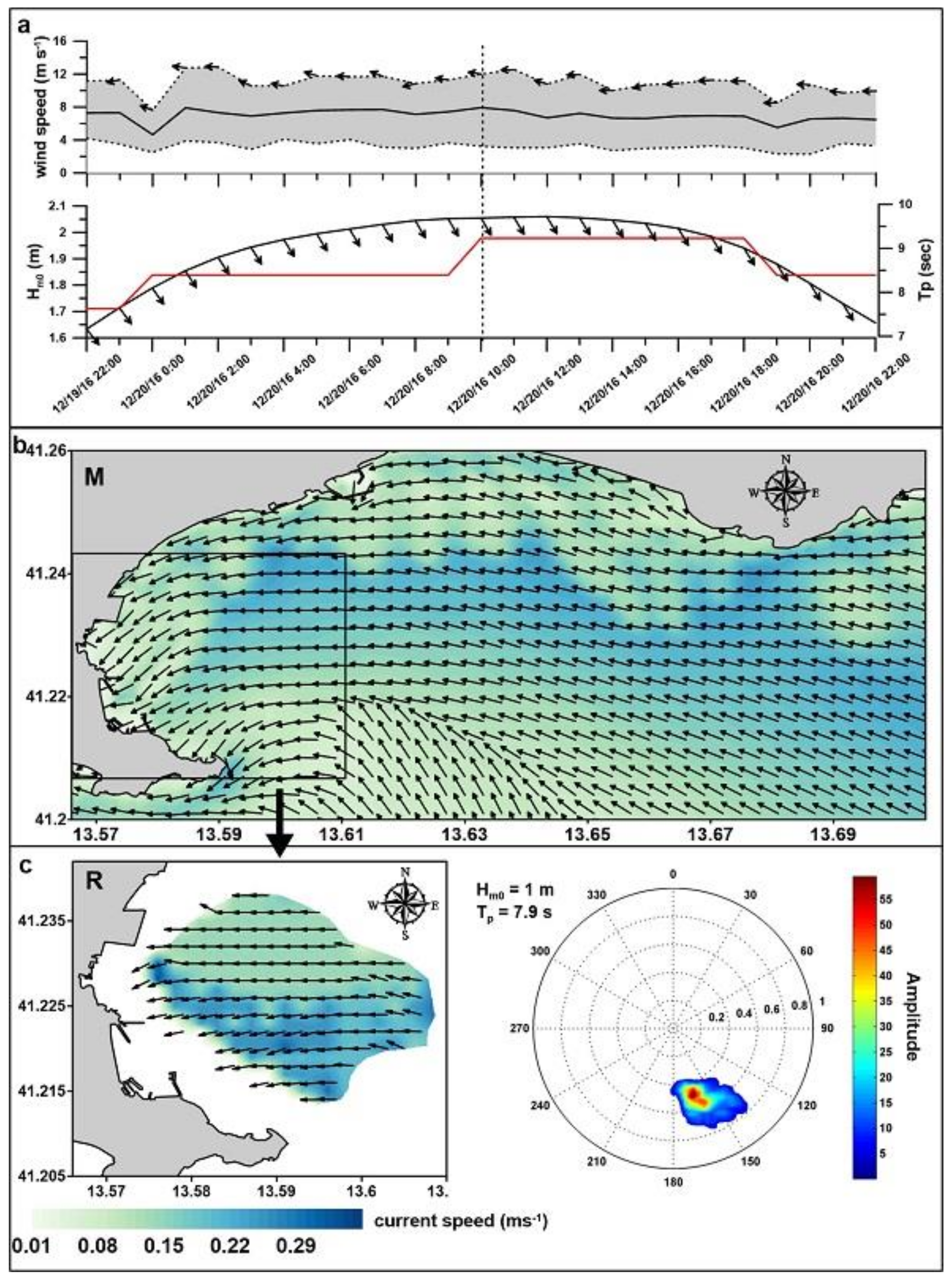
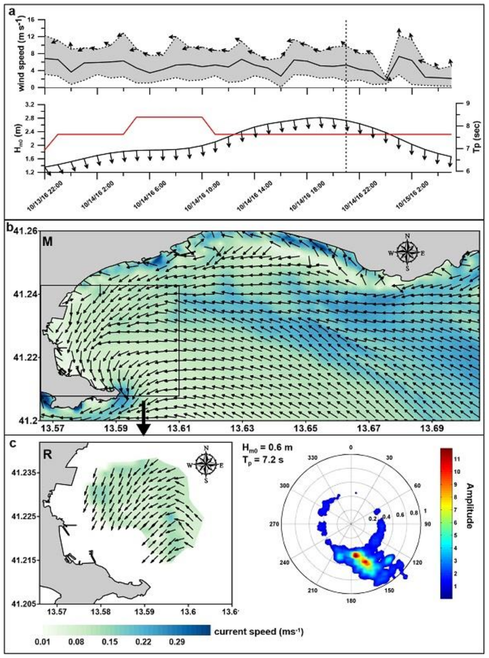
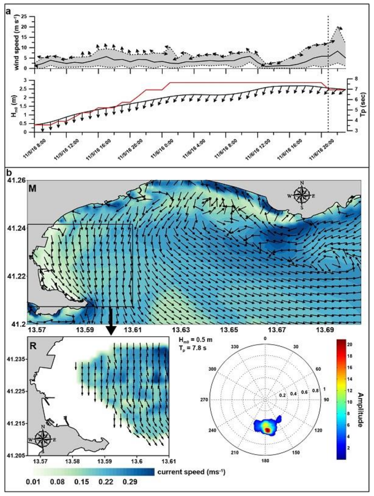
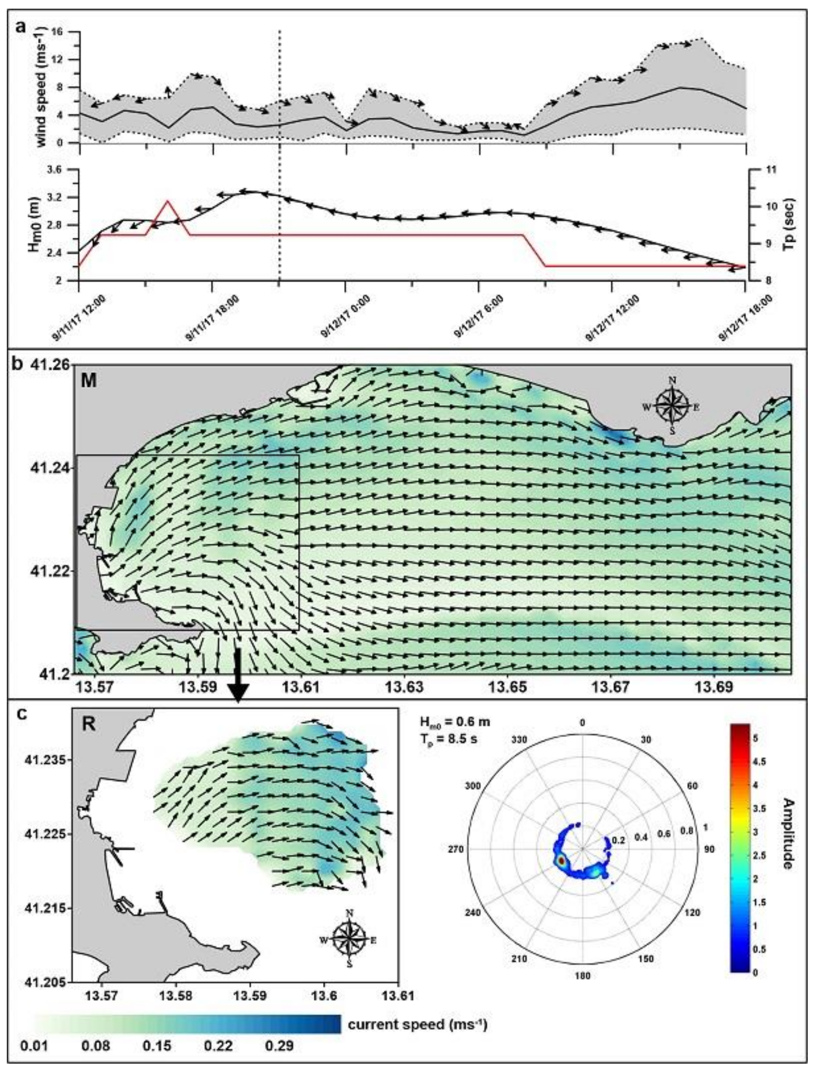
3.1. Analysis of Storms

The wind records at Ponza and Gaeta port (Figure 2a,b) are dominated by wind from the northeast (NE) and west (W), while at Punta Stendardo the prevailing directions involve eastern and western sectors (Figure 2c). Inside the gulf, W and northwest (NW) winds are side-shore and offshore, while the NE and southeast (SE) directions are nearly perpendicular to the coastline.

The wave records of a 20-year time series of the Ponza Island buoy show prevailing western events (Figure 3a). The morphology of the Gulf of Gaeta and the presence of Ischia Island constrain the propagation of waves from a small southeast (SE) sector that determine a local wave climate inside the gulf that shelters the coast from the main western events. This behavior is highlighted by the records of the wave buoy inside the gulf (Figure 3b) where the waves are less intense and exclusively come from eastern and southeastern sectors, due to wave refraction.

The storm events on the Ponza dataset were selected using the methodology of Mendoza et al. [65] available for the Mediterranean Sea. A storm is defined as an event when the wave height exceeds the threshold of two meters for more than 6 h. The storm events, coming from a directional sector between 120° N and 300° N, were extracted from the wave buoy time series of Ponza. The selected storm events from the Ponza dataset have an annual mean frequency of 10% and are distributed seasonally throughout the year with a decreasing trend proceeding from winter toward summer (31% in autumn, 38% in winter, 25% in spring and 6% in summer). The distribution of storm directions shows a nearly unimodal shape and do not show significant seasonal behavior [66].

In the western Mediterranean Sea, the cyclogenesis area is essentially composed of sub-synoptic lows, which are triggered by the major North Atlantic synoptic systems as affected by local orography [39]. The typical situation is characterized by a low-pressure system that develops in the Gulf of Genoa, with synoptic northerly flow impinging on the mountain ranges and being funneled between the Alps and Massif Central [67]. Moreover, cyclogenesis over different areas can consecutively occur as the result of the same synoptic system crossing central Europe. Especially in winter, there is a prevailing south-eastward direction of the cyclone track that extends through Italy down to the Albanian and Greek coasts. This synoptic condition contributes to limiting the wavefield’s seasonal variability in the study area and identifies semi-permanent forcing [66]. These forcing are associated with the strong westerly winds channeled by the Strait of Bonifacio and induced circulation features such as the North Tyrrhenian Cyclone and North Tyrrhenian Anticyclone [68]. Storm classes are determined by a statistical approach using k-means clustering algorithms. The clustering aims to group multivariate wave data into n number of classes in an optimized manner such that dissimilarity between cluster groups is maximized. K-means are currently one of the principle cluster methods used to characterize wave climates for coastal engineering applications [53,69,70]. K-means algorithms finds the optimal Voronoi cells in uni- or multi-dimensional datasets for k-clusters and returns a centroid for each cluster. Voronoi cells take the form of irregular polyhedra, and describe the multi-dimensional space occupied by each cluster. Voronoi cells are determined by minimizing the sum of dissimilarities (squared errors) between each object and its corresponding centroid. The centroid is not an actual observation in the dataset; rather, it is an average value which acts as the central reference point for each cluster. The dataset used for the clustering process does not consider summer events, which are rare and differ from typical storms. Once storm events were selected, k-mean clustering was performed on Tp/Dir, which are the parameters primarily influenced by the generation source of waves, while wave height was not used because it is less variant across all directional sectors. The best fit of k-means clustering recognizes two well-defined groups (Figure 4a,b) in which silhouette values were maximized. The first group has a well-defined peak characterized by dominant western events and is named the Western Class (WC), while the secondary group is characterized by less frequent southerly direction events (SDC). This secondary group corresponds to the orientation of the opening sector of the gulf. In this group, multiple small peaks are present in the distribution and the wave field is separated by a Gaussian Mixture Model (GMM) to decompose multiple wave geneses [71]. The analysis of SDC reveals three clusters separated in terms of direction (Figure 4c).

The wave field originating from single classes is analyzed in the form of joint probability density (JPD) functions (Figure 5) to highlight the characteristics of classes. The wave field of the main two classes (Figure 5a) produced by storms highlights the genesis of different waves with characteristic wave periods. The WC events are characterized by a larger probability of longer waves (8.2 s) with respect to the SDC events (6.7 s). The GMM clustering of SDC (Figure 5b) events highlight that the characteristics of waves produced during these storms are similar, suggesting that differences are only constrained by the incident angle of waves that drive different coastal circulations. On this basis, 4 different classes (WC and the three sub-classes of SDC) were recognized and respectively named the Western Class (WC), Southwestern Class (SWC), Southern Class (SC) and Southeastern Class (SEC), and the dynamic induced by these events is described through the numerical model simulations and X-band radar records.

The wave parameters associated with the maximum JPD probability (red contours of Figure 5) of each storm class are reported in

Table 2. Characteristics of storm classes.

Parameters	WC	SDC
		SWC	SC	SEC
Dir (°N) +/− StD	259° +/− 16°	223° +/− 3°	185° +/− 19°	134° +/− 6°
Hm0 (m)	2.3	2.2	2.2	2.2
Tp (second)	8.2	6.7	6.7	6.7
Frequency (%)	68	7.5	18	6.5

.

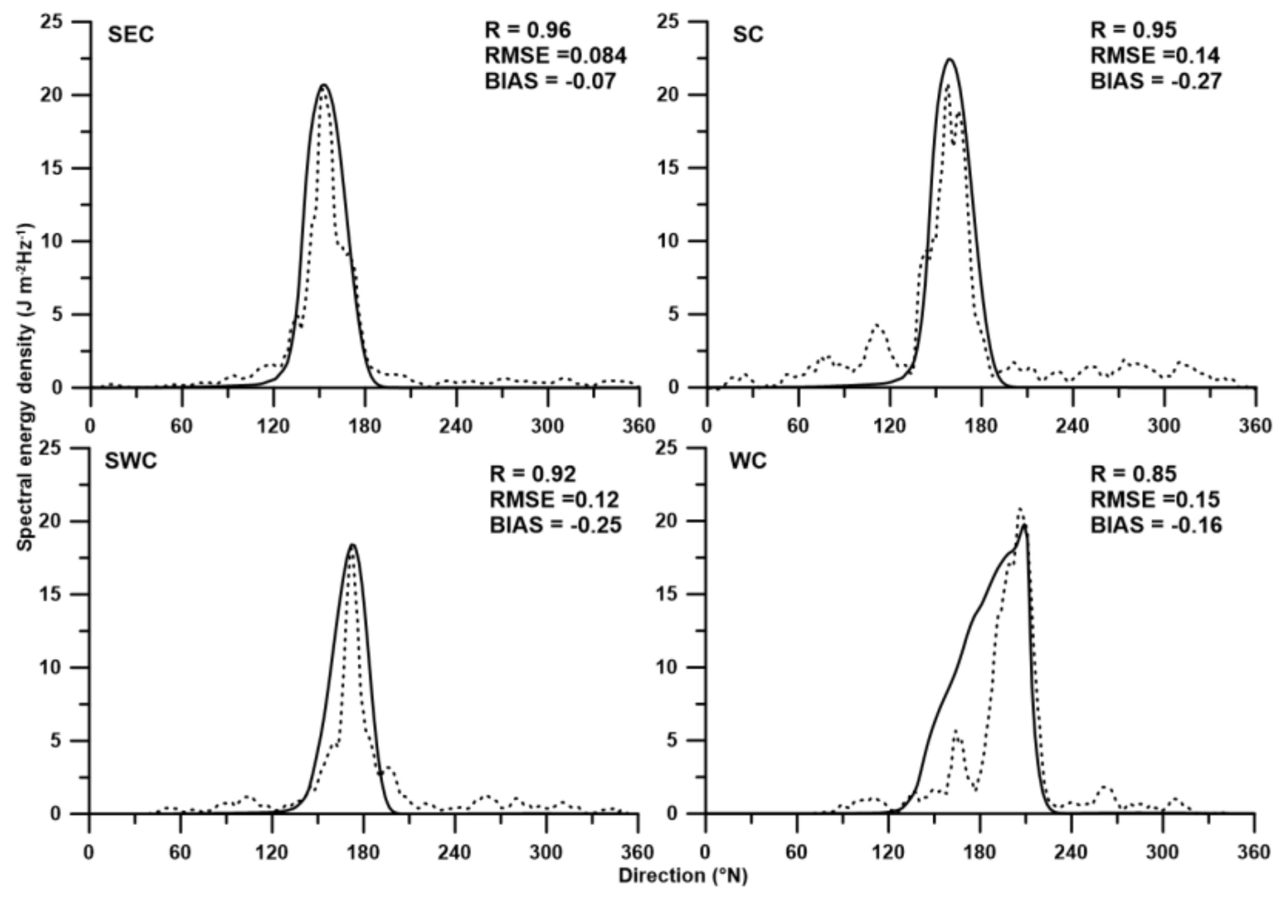
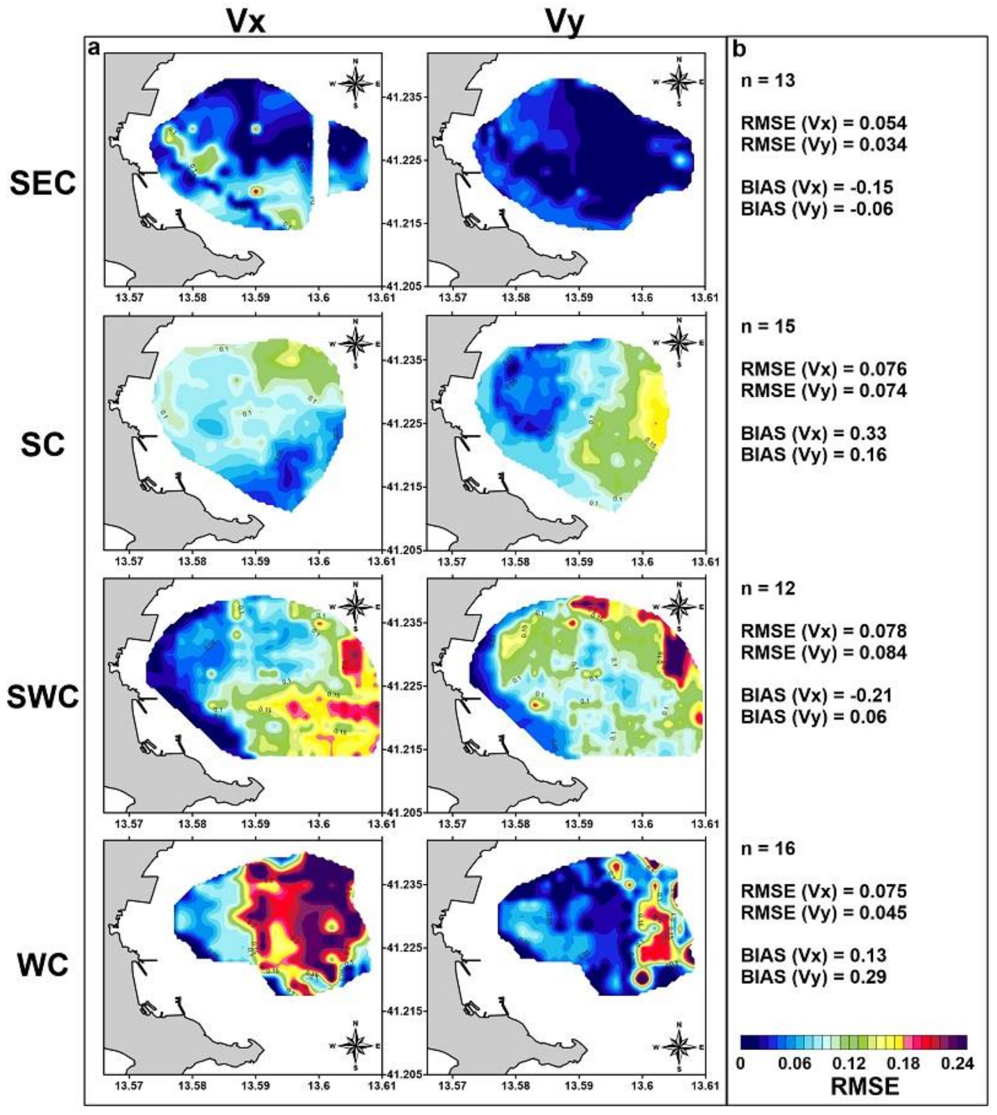
3.2. Coastal Circulation Induced by Storm Classes

The study area is protected by coastal morphology to prevailing western events, and measurement capability has many important limitations. Nevertheless, during the operating period of the X-band radar, four storms belonging to storm classes were recorded. In particular, four periods were simulated (13–15 October 2016, 5–6 November 2016, 19–20 December 2016 and 10–12 September 2017), representing historical events that are substantially closer to the centroid conditions of storm classes. The comparison between model results and radar records involve both surface currents and wave spectra and derived statistical parameters (significant wave height, SWH).

The wave spectra quadratic mean of the model and radar show good agreement (Figure 6) for all storm classes with slight discrepancies in WC events. The SWH comparison conducted for the all events shows tight correlation (R = 0.87; RMSE = 0.34 and BIAS = −0.35) between the measured and model data.

The contour fill map of the RMSE and average RMSE and BIAS highlight the discrepancy between the radar measurements and the model results in different storm classes for the surface currents (Figure 7). The statistics show good correspondence between radar acquisitions and model results, especially for SEC and SC classes. When the waves approach the coast more obliquely, in the cases of SWC and WC classes, there is a greater discrepancy, especially for the x component.

For the SEC, an event of two days (19–20 December 2016) occurred with a maximum SWH, offshore from the Gulf, of 2.1 m with a peak period of 9 s (Figure 8a). This event had a constant easterly wind with an average intensity of approximately 8 ms⁻¹. Radar measurement (R) corresponding to the peak of the event (Figure 8c) showed a westward current with an increasing gradient proceeding southward. The numerical model result (M) (Figure 8b), which is the result of the combined effect of wind and waves, had correspondence with R and highlights that the flow was primarily directed westward, entering with a slight rotation within the gulf. The maximum intensity on the surface layer was 0.23 ms⁻¹, and maximum values were observed in correspondence with Monte Scauri and Punta Stendardo as well as in the central portion of the gulf. Waves that propagate inside the gulf have SWH of 1 m and Tp of 7.9 s. The wave spectrum covers a wide range of directions from 140 to 180° N with a peak placed at 160° N that differs from offshore incident waves by approximately 20°.

An event belonging to SC occurred on 13–15 October 2016, during which a maximum SWH, offshore from the Gulf, reached 2.8 m and a 7.5-s peak period was observed (Figure 9a). During this event, the wind came from the ENE and ESE directions with an average intensity in a range of 4–8 ms⁻¹. R measurements in correspondence with the peak of the event (Figure 9c) show currents with an intensity of approximately 0.07–0.15 ms⁻¹ that progressively rotate while approaching the coast parallel to the shoreline. The M result (Figure 9b) shows currents directed toward the NW that rotate approaching nearshore following the morphology of the gulf. The maximum intensity of the surface currents is observed in correspondence with Monte Scauri and Punta Stendardo (0.24 ms⁻¹), and their magnitude generally decreases when entering the gulf. Waves that propagate inside the gulf have SWH of 0.6 m and Tp of 7.2 s. The wave spectrum covers a wide range of directions from 140 to 190° N with a peak placed at 170° N.

An event belonging to SWC occurred on 5–6 November 2016, during which a maximum SWH, offshore the Gulf, reached 2.6 m and there was a 7.6-s peak period (Figure 10a). R measurements highlight a current with an intensity between 0.05 and 0.2 ms⁻¹ that is oriented southerly in the presence of wind from the west (Figure 10c). The modelled nearshore flow on the western side of the gulf proceeds southerly and proceeding toward east the currents turn eastward (Figure 10b). Waves that propagate inside the gulf have SWH of 0.5 m and Tp of 7.8 s. In this case, the wave spectrum covers a range of directions from 160 to 190° N with the peak placed at 180° N.

An event belonging to WC occurred on 11–12 September 2017 during which a maximum SWH, offshore the Gulf, reached 3.4 m and there was a 9-s peak period (Figure 11a). During this event, the wind spread from the NW and W with an average intensity in a range of 2–8 ms⁻¹. R measurements corresponding to the peak of the event (Figure 11c) show currents with an intensity of approximately 0.08–0.2 ms⁻¹ oriented toward the east that progressively rotate to the SE moving eastward. The numerical model result (Figure 11b) agrees with the R measurements highlighting a flow oriented from west to east with an intensity of approximately 0.04–0.2 ms⁻¹ with the maximum located in the nearshore zone. Waves that propagate inside the gulf have SWH of 0.6 m and Tp of 8.5 s. The wave spectrum has a bimodal shape and covers a wide range of directions from 270 to 120° N with the peak placed at 240° N.

The ability of the different storm classes to trigger sea-bed sediment resuspension has been evaluated from the model considering the maximum bed shear stress (Figure 12) in correspondence of the peak of the events, belonging to the different storm classes. To select the bed shear stress threshold useful to describe the resuspension occurrence, two sediment sizes (0 and 5 phi) according to the characteristics of the seabed within the gulf have been considered (as previous described in paragraph 2.1). The theoretical bed shear stress thresholds for coarse sand and coarse silt have been retrieved from critical shear stress table of USGS [72]. The bed shear stress computation used in the model is referred to the Fredsoe formulation as reported by Soulsby et al. [73]. The storm classes SEC, SC and SWC can trigger resuspension within the gulf especially in the nearshore sector of the eastern side of the gulf where the bed shear stress reaches the threshold of motion of sandy fraction. In proximity of Stendardo jetty the shear at the bed is not enough intense to cause resuspension. On the contrary, WC events are not able to trigger resuspension within the gulf except at east of Formia port where starts the movement of coarse silt fraction.

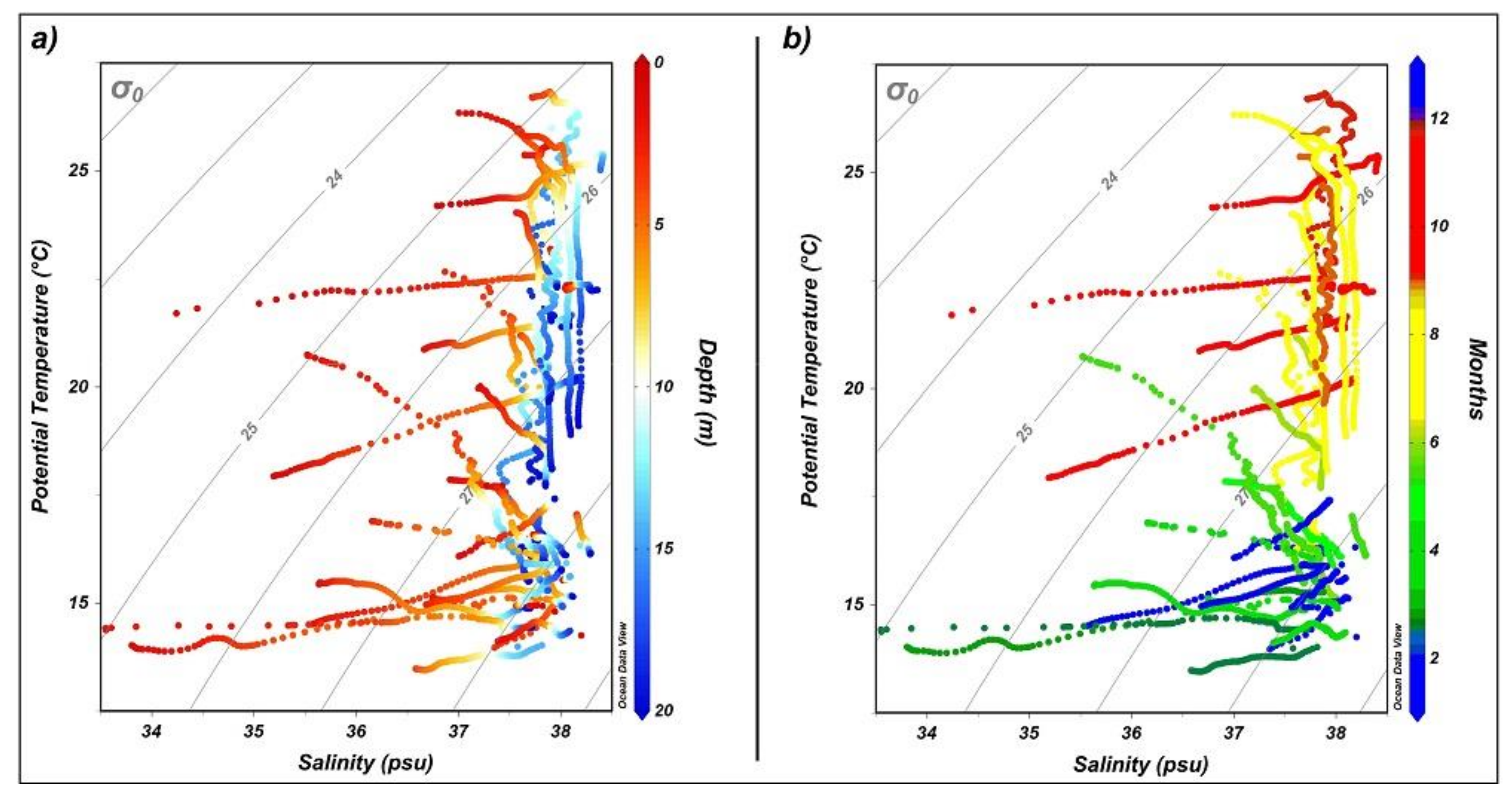
3.3. Analysis of CTD Profiles

The T-S diagrams obtained during 5-years (2013–2017) monthly CTD profiles show the relative influence of salinity and temperature on the density structure of the water column at the sampling point within the gulf (Figure 13). Salinity drive the density structure of the upper layer (Figure 13a) especially during Autumn and Winter period when minimum values were recorded 34–35 psu (Figure 13b). This process is variable during the year; in winter it reaches 7 m depth while in summer involve only a thick surface layer. On the contrary, in all the seasons the temperature influences the density structure of the deeper layer below 10 m depth where the salinity is constrained between 37.5 psu and 38 psu.

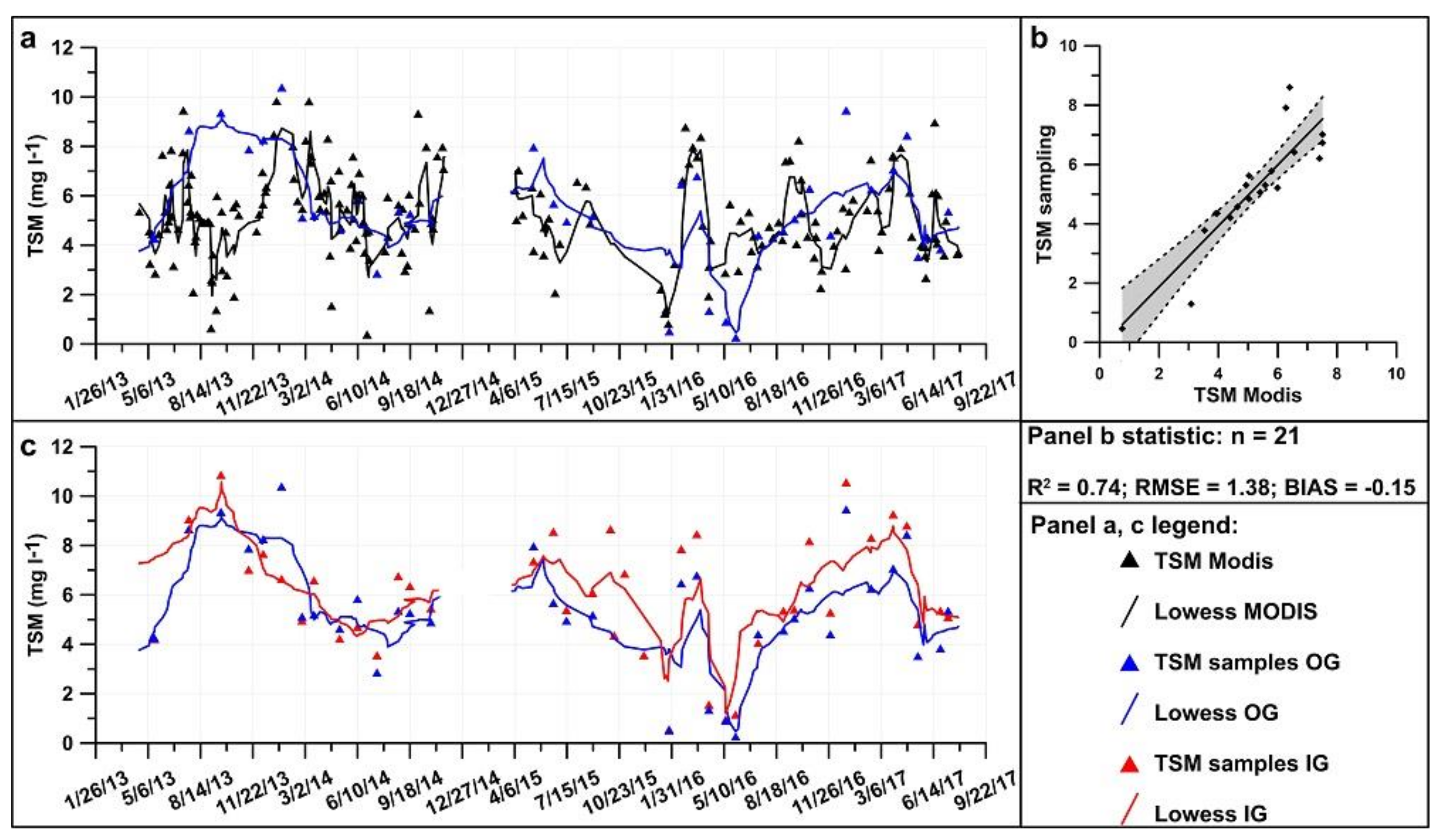
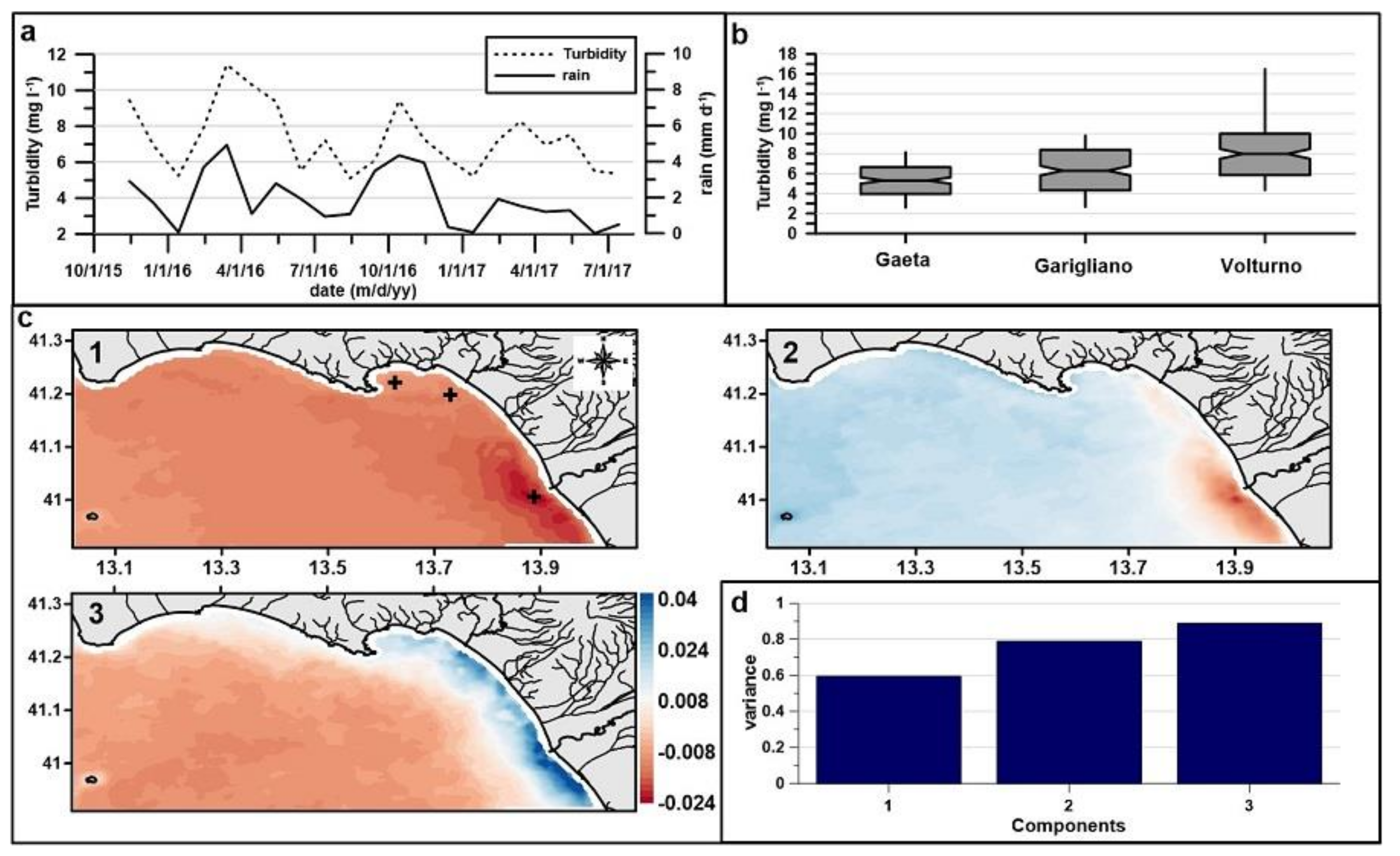
3.4. Regional Assessment of SPM Concentration

The outside gulf (OG) samples were compared with the suspended solid concentration extracted from satellite-derived SPM. Water sampling on the OG stations indicates a good correspondence with SPM determined from MODIS imagery processing, as demonstrated by a statistical index obtained in comparison (Figure 14b). The time series of sampling performed inside and outside the gulf indicates a value of SPM concentration ranging from 0.1 to 11 mg L⁻¹ and an average value of between 4 mg L⁻¹ and 8 mg L⁻¹. A systematic gap of turbidity of approximately 1–2 mg L⁻¹ is also visible inside the gulf, as is a clear seasonal fluctuation that involves both sampling stations.

To evaluate the contribution of continental inputs on SPM distribution within the study area, the total available pluviometric records from the stations of Figure 1 were correlated with the SPM concentration acquired by a turbidimeter placed within the gulf of Gaeta. Figure 15a shows the agreement (R = 0.64; p-value < 0.01) between the monthly mean of rain and SPM concentration. Rainfall monthly mean is computed considering all pluviometric stations within the catchment area (Figure 1) and represents the continental inputs contribution. To characterize the water turbidity condition along the coastal area, the SPM concentration was extracted from three points of satellite imagery (cross mark on pattern 1 of Figure 15c), respectively, in front of the Volturno and Garigliano river mouths and within the Gulf of Gaeta. The distributions of SPM concentration (Figure 15b) highlight the decreasing trend of turbidity moving from the Volturno River to the Gulf of Gaeta.

The regional variability in the suspended particulate matter concentration can be assessed using EOF analyses, which provide a compact description of the spatial and temporal variability of data series in terms of statistic modes, where most of the variance of the spatially distributed parameters can be observed in the first few orthogonal functions [74]. The distribution patterns were reconstructed starting from a time series of MODIS imagery collected from 2013 to 2017 (n = 630). The time series was analyzed through the EOF while selecting components that describe 90% of the variance. The results of the EOF analysis suggest that the variance on the study area at the regional scale is dominated by the variability of the river plume of the Volturno River, which appears to be the primary factor that controls the turbidity level on the coastal area. The three patterns of Figure 15 represent 90% of the variance (Figure 15b) and can be attributable to a seasonal dynamic of the plume (pattern 1 of Figure 15a) as well as to a contribution of other coastal rivers such as the Garigliano (patterns 2–3 of Figure 15a). As observed from the three observation points, the three patterns highlight an along-shore gradient.

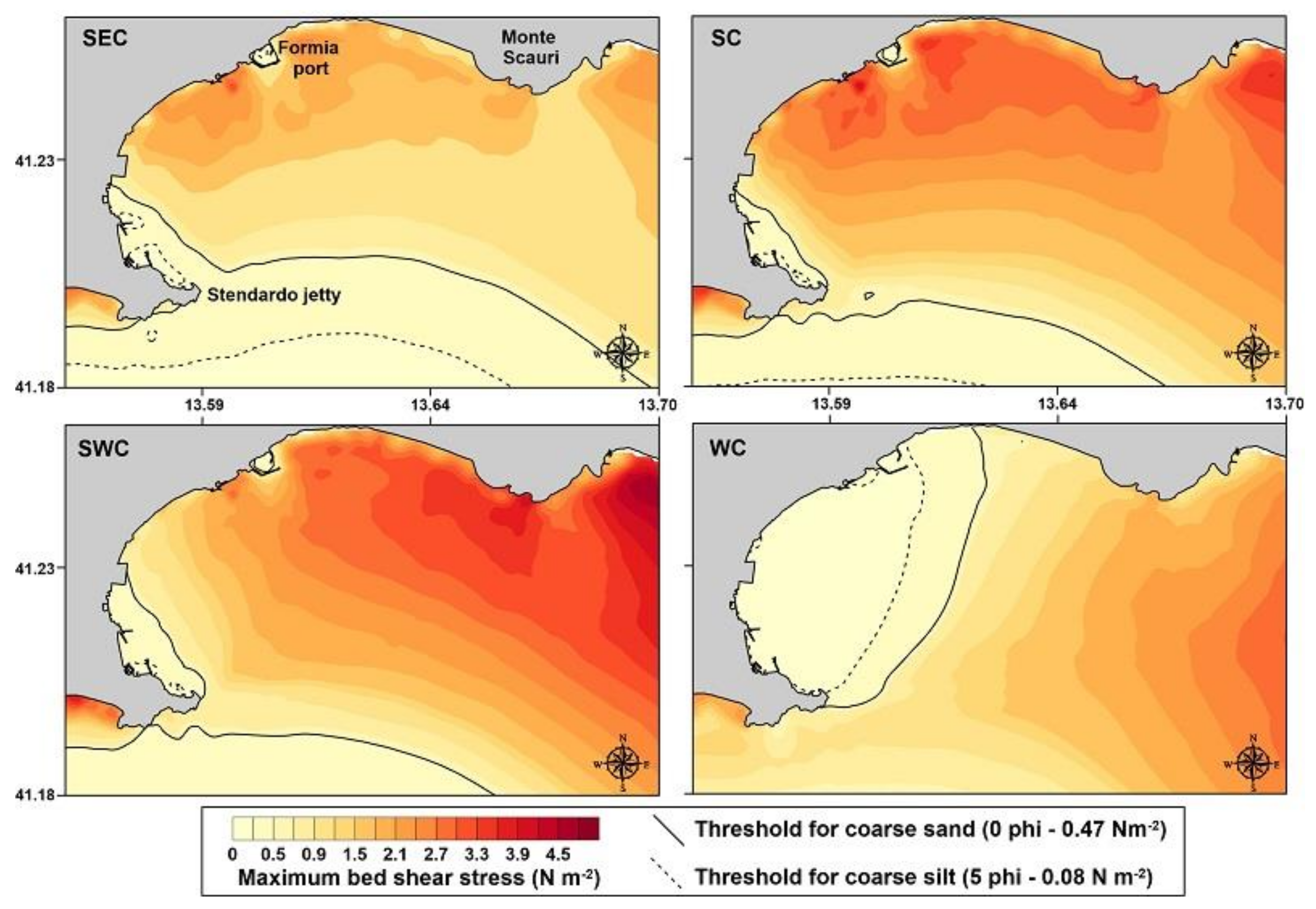
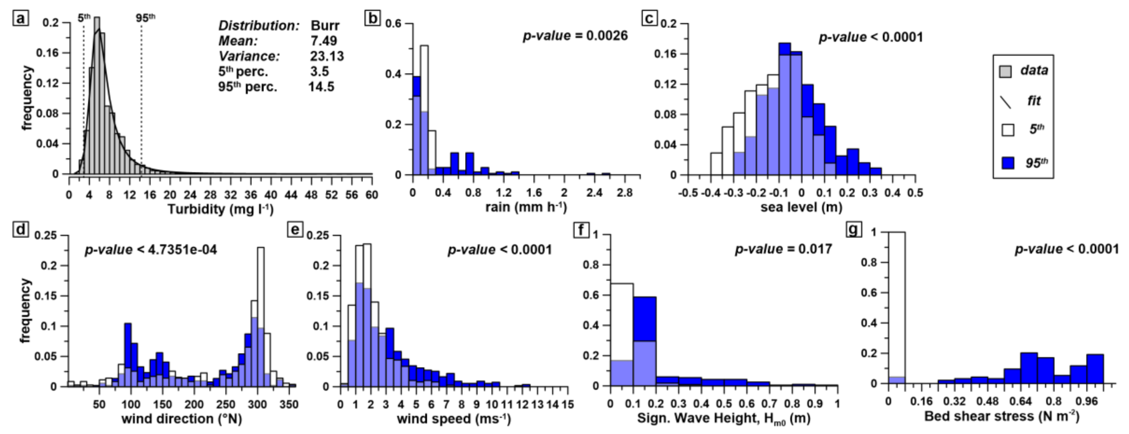
3.5. Analysis of the Response of Local Turbidity to the Main Physical Forcing

The analysis aims to detect the possible relationship, at the local scale, between the H and L levels of the SPM concentration recorded within the gulf as well as the dynamic factors. The dynamic factors used for the analysis are: SWH recorded by radar, the wind speed and direction measured by meteorological station, sea-level collected by marigraph and precipitations collected by pluviometers within the catchment area. Moreover, the bed shear stress computed by model which is the result of combined action of wind and waves has been considered. The distributions of the dynamic factors associated with the high (H) and low (L) level of the SPM concentration were statistically compared in pairs using the Wilcoxon signed-rank test. The analysis acknowledged statistical dissimilarities between the distributions associated with L and H for all considered dynamic factors. Furthermore, the results uncover important evidence: only intense rain events (Figure 16b) are associated with H events, while nearly all the L events are associated with scarce precipitations. Tides within the Gulf of Gaeta (Figure 3d) show a semi-diurnal tidal cycle with a range of maximum 0.2 m, and the distribution of sea level shows a mode of approximately −0.05 m. Distributions in sea level highlight the asymmetry of H events toward a high stand of the sea, and the distribution of sea level shifts toward a negative value during L events. The difference between the two distributions involves the water level exceeding the range of the tidal excursion. The wind direction (Figure 16d) shows that events coming from SE (onshore) occurs more frequently during H, while events from the NW (offshore) are more frequently associated with L. The distributions of wind speed (Figure 16e) show that intense wind (wind speed > 6.5 ms⁻¹) is always associated with H events, while weak wind is more frequently associated with L events. Figure 16f shows how H corresponds with greater wave intensity, while L indicates calm seas. Lastly, distributions of modelled bed shear stress (Figure 16g) highlight the correspondence of high value to H turbidity while transparency condition occurs always below 0.08 Nm⁻².

These data were confirmed by correlation analysis in which statistical correspondence was found between turbidity and dynamic factors except for wind speed, as reported in

Table 3. Pearson correlation analysis results between turbidity and dynamic factors.

Dynamic Factors	R	p-Value
Sea Level (m)	0.62	<0.01
SWH (m)	0.46	<0.01
Bed shear stress (Nm−2)	0.73	<0.01
Rain	0.75	<0.01
Wind direction (°N)	−0.47	<0.01
Wind speed (m/s)	−0.06	0.54

. The SWH, sea level, wind speed and direction correlation analysis were performed each 20 min while the comparison with rainfall was carried out hourly.

Sea level, SWH, bed shear stress and rain show direct correlation, demonstrating that positive set-up, wave intensity, bed shear stress of currents and rain favor an H level of turbidity. Wind direction shows an inverse correlation, demonstrating that westerly and northwesterly winds (270–330° N) that blow offshore in the study site correspond to L turbidity with respect to those events from the east and southeast (90–160°), which are linked to an H level of turbidity.

4. Discussion

The coastal morphology of the Gulf of Gaeta is naturally sheltered from the prevailing events, which causes a generally weak hydrodynamism within the gulf, as demonstrated by the fine particle sediments of the seabed [13,39]. The coastal dynamic of the area and the main conditions that affect the suspended particulate matter (SPM) distribution are poorly understood. Nevertheless, the multiple coastal conflicts among natural resources and human activities warrant detailed investigations into the coastal dynamic processes that drive the accumulation and dispersion processes of contaminants. This study was the first to investigate the dynamic of the Gulf of Gaeta with a focus on the dynamic processes that affect fine particle concentrations within a coastal site. The study was conducted using a multidisciplinary approach that involved remote sensing acquisitions, in situ measurements and numerical modelling. Because high energetic events are the main factor responsible for coastal processes on a short time scale, the storms in the coastal area were classified using a clustering procedure. The hydrodynamic conditions in the study area are tightly linked to the regime of storms, which trigger different patterns of circulation within the gulf [75]. The analysis of the storm reveals four classes (South-East Class, SEC; South Class, SC; South-Western Class, SWC and Western Class, WC) that are characterized by the presence of different waves with characteristic wave periods. The effect of these storm events on the hydrodynamic and wave fields within the study area was reproduced using DELFT3D-FLOW and SWAN. A comparison with X-band radar acquisitions highlighted a tight correlation between the predicted and measured data, both in terms of surface currents (x and y components of velocity) and wave parameters (wave spectra and SWH). Nevertheless, the discrepancy was higher in the western events (SWC and WC) as the models were forced with wind and wave data coming from a single point, which is not adequate to represent the high spatial variability of the meteomarine conditions due to coastal and continental morphology. Data from atmospheric and wave models at high spatial resolution will be used to feed DELFT3D-FLOW and SWAN and thus improve the predictive performance of the models. The model results show that southern events (SEC, SC, WSC) promote resuspension within the gulf and circulation favor the accumulation of water masses on the coast. These events that perpendicularly impact the coast are responsible for the largest waves entering the gulf, and positive sea level set-up, especially for SEC, is linked to high turbidity phenomena as well as the triggering of resuspension processes, as widely observed in other coastal sites [76,77,78]. In contrast, the WC conditions are not able to trigger resuspension and the circulation cause a displacement of water masses in the offshore zone. west (W) and north-west (NW) events moving surface water masses away promote greater transparency and water renewal [79]. In the short term, local variations may be explained by peaks in wave height or fluvial input, and wind direction plays a primary role in modulating the turbidity of the water, as observed in other sheltered coastal sites where wind is a primary factor for circulation and suspended sediment concentrations [37,38,80] and also controls the movement of the river plume [75]. The analysis of SPM derived from MODIS imagery as well as the correspondence between rain records and turbidity reveal the primary influence of the nearby river controlling the distribution of SPM at the regional scale. The distribution patterns observed by the EOF analysis can be considered long-term distribution influenced by the time-average river load and by the balance between convergent residual circulation and the spreading effects of horizontal dispersion [81]. The near-bed residual current causes a net flux of SPM and accumulation of fine sediment in a narrow coastal strip of several km [82]. The first pattern of EOF shows that the area influenced by the river plume extends northwestward, rounding Punta Stendardo. The transport of sediments coming from the Volturno and Garigliano rivers over Punta Stendardo was demonstrated by previous mineralogical and radionuclide investigations, highlighting a preferentially SE-NW transport of sediments that was also confirmed by more recent hydrological measurements [83]. These sediments can reach the northern beaches up to Monte Circeo [84]. Water sampling at inside gulf (IG) and outside gulf (OG) stations indicate an average SPM concentration in a range of 4-8 mg L⁻¹. The results highlight a constant gap of increasing turbidity within the gulf between OG and IG and can be explained by the combined effect of multiple factors including also human activities within the gulf, which may increase the suspended solid matter supply. In the long term, changes in the soil use can be related to an increase in the fine fraction supply [85,86,87]. The dynamic of the gulf leads to a favorable area of accumulation of fine sediments coming from the mainland especially during the prevailing western events. Precipitation in the Western Mediterranean is strongly influenced by cyclones and global atmospheric patterns, in particular during winter, by the North Atlantic Oscillation (NAO) [88,89]. The association between the structural characteristics of cyclones and NAO was demonstrated by Trigo et al. [90] and during the last fifty years the cyclones have decreased in the Western Mediterranean Sea and in the same way, the Mediterranean average winter precipitation [91]. This condition influence both the dynamic processes induced by storms within the gulf and the river discharges with an impact on the sedimentary balance of the coastal zone. Since each storm type is potentially caused by different large scale synoptic pressure system, climate change may induce long-term variation to circulation patterns. The fresh water advection within the gulf is confirmed by the water column investigations which highlight the main role of salinity on the variations of the water column density structure in the surface layer. Minimum salinity values occur during autumn and winter season, period with maximum precipitation and consequent run-off. The surface layer salinity is constantly less than deeper layer which agree with general characteristics of Tyrrhenian basin where the salinity ranges between 38.2 psu and 38.4 psu [92]. The dynamic of the river plumes is affected mainly by density structure and the vertical mixing of SPM is slow especially in stratified waters and in low energy environment as the sheltered coastal area [81,93] where mixing factors are weak. This condition is also confirmed by the results of previous studies on the effect of fish farming within the gulf, which limits the dispersion to 1 km upstream [94,95,96]. Future developments will concern the implementation of a water quality model in the study area as well as a balance between resuspension and settling of particles can be developed. A direct estimate of the sedimentary river contribution will be carried out as well as an analysis of the salinity distribution along the study area that will allow to analyze in more detail the estuarine dynamic processes.

5. Conclusions

In this multidisciplinary approach, we investigate the coastal dynamics of the Gulf of Gaeta. The X-band radar system supports the analysis of the dynamic processes of the SPM concentration providing a large dataset useful for the hydrodynamic model’s validation. The Gulf of Gaeta is subjected to natural siltation, which is fed by the river contributions. South-eastern winds push the plume towards the Gulf of Gaeta, and the coastal morphology favors retention of the SPM. Short-term high and low fluctuations in SPM concentration within the gulf are triggered by the local effect of wind induced circulation and wave intensity. In particular, the direction of events and bottom sediment resuspension play a key role in modulating the SPM concentration in the study area. Microtidal excursion play a minor role on turbidity variation in this area, while fluvial discharge, wind direction and wave height result to be more important. In the short-term, sediment handled during dredging activities can alter the SPM supply within the gulf, and while the fine particles have a greater probability to remain confined during events from the south, western events favor a faster dispersion. Consequently, the results of our study highlight the need to link SPM concentration to the meteorological conditions that can amplify or dampen the local concentrations of material handled during dredging activities. The multidisciplinary approach hereby presented can be transferred to other coastal areas to improve coastal management strategy. The adopted methodology leads to long-term observation of coastal dynamic processes which is a fundamental issue in the climate change perspective.

References

1. Lotze, H.K.; Lenihan, H.S.; Bourque, B.J.; Bradbury, R.H.; Cooke, R.G.; Kay, M.C.; Kidwell, S.M.; Kirby, M.X.; Peterson, C.H.; Jackson, J.B.C. Depletion, degradation, and recovery potential of estuaries and coastal seas. Science 2006, 312, 1806–1809. [Google Scholar] [CrossRef] [PubMed]
2. Jones, S.J.; Frostick, L.E. (Eds.) Sediment Flux to Basins: Causes, Controls and Consequences; Special Publications; Geological Society: London, UK, 2002; Volume 191, p. 284. [Google Scholar]
3. Burt, T.; Allison, R. Sediment Cascades: An Integrated Approach; Wiley-Blackwell: Chichester, UK; Hoboken, NJ, USA, 2010; p. 482. [Google Scholar]
4. Macias, D.; Garcia-Gorriz, E.; Stips, A. Major fertilization sources and mechanisms for Mediterranean Sea coastal ecosystems. Limnol. Oceanogr. 2017. [Google Scholar] [CrossRef]
5. Mann, K.H.; Lazier, J.R.N. Dynamics of Marine Ecosystems: Biological–Physical Interactions in the Oceans; Black Well Scientific Publications, Inc.: Boston, MA, USA, 1991. [Google Scholar]
6. Careddu, G.; Costantini, M.L.; Calizza, E.; Carlino, P.; Bentivoglio, F.; Orlandi, L.; Rossi, L. Effects of terrestrial input on macrobenthic food webs of coastal sea are detected by stable isotope analysis in Gaeta Gulf. Estuar. Coast. Shelf Sci. 2015, 154, 158–168. [Google Scholar] [CrossRef]
7. Montefalcone, M.; Vassallo, P.; Gatti, G.; Parravicini, V.; Paoli, C.; Morri, C.; Bianchi, C.N. The exergy of a phase shift: Ecosystem functioning loss in seagrass meadows of the Mediterranean Sea. Estuar. Coast. Shelf Sci. 2015, 156, 186–194. [Google Scholar] [CrossRef]
8. Serrano, O.; Lavery, P.; Masque, P.; Inostroza, K.; Bongiovanni, J.; Duarte, C. Seagrass sediments reveal the long-term deterioration of an estuarine ecosystem. Glob. Chang. Biol. 2016, 22, 1523–1531. [Google Scholar] [CrossRef] [PubMed]
9. Myers, N.; Mittermeier, R.A.; Mittermeier, C.G.; da Fonseca, A.B.; Kent, J. Biodiversity hotspots for conservation priorities. Nature 2000, 403, 853–858. [Google Scholar] [CrossRef] [PubMed]
10. Blanton, J.O. Ocean currents along a Nearshore Frontal Zone on the Continental Shelf of the Southern United States. J. Geophys. Res. 1981, 11, 1627–1637. [Google Scholar]
11. Gelfenbaum, G.; Stumpf, R.P. Observations of currents and density structure across a buoyant plume front. Estuaries 1993, 16, 40–52. [Google Scholar] [CrossRef]
12. Dinnel, S.P.; Schroeder, W.W.; Wiseman, W.J., Jr. Estuarine-shelf exchange using Landsat images of discharge plumes. J. Coast. Res. 1990, 6, 789–799. [Google Scholar]
13. Hickey, B.M.; Pietrafesa, L.J.; Jay, D.A.; Boicourt, W.C. The Columbia River plume study: Subtidal variability in the velocity and salinity fields. J. Geophys. Res. 1998, 103, 10339–13368. [Google Scholar] [CrossRef]
14. Marques, W.C.; Fernandes, E.H.; Monteiro, I.O.; Moller, O.O. Numerical modeling of the Patos Lagoon coastal plume, Brazil. Cont. Shelf Res. 2009, 29, 556–571. [Google Scholar] [CrossRef]
15. Kourafalou, V.H.; Stanev, V.E. Modeling the impact of atmospheric and terrestrial inputs on the western Black Sea coastal dynamics. Ann. Geophys. 2001, 19, 245–256. [Google Scholar] [CrossRef]
16. Ollivier, P.; Radakovitch, O.; Hamelin, B. Major and trace elements partition and fluxes in the Rhone river. Chemical Geology, in preparation. Chem. Geol. 2011, 285, 15–31. [Google Scholar] [CrossRef]
17. Radakovitch, O.; Roussiez, V.; Ollivier, P.; Ludwig, W.; Grenz, C.; Probst, J.L. Particulate heavy metals input from rivers and associated sedimentary deposits on the Gulf of Lion continental shelf. Estuar. Coast. Shelf Sci. 2008, 77, 285–295. [Google Scholar] [CrossRef] [Green Version]
18. Boldrin, A.; Langone, L.; Miserocchi, S.; Turchetto, M.M.; Acri, F. Po River plume on the Adriatic continental shelf: Dispersion and sedimentation of dissolved and suspended matter during different river discharge rates. Mar. Geol. 2005, 222–223, 135–158. [Google Scholar] [CrossRef]
19. Turritto, A.; Acquavita, A.; Bezzi, A.; Covelli, S.; Fontolan, G.; Petranich, E.; Piani, R.; Pillon, S. Suspended particulate mercury associated with tidal fluxes in a lagoon environment impacted by cinnabar mining activity (northern Adriatic Sea). J. Environ. Sci. 2017, in press. [Google Scholar] [CrossRef]
20. Oursel, B.; Garnier, C.; Zebracki, M.; Durrieu, G.; Pairaud, I.; Omanovic, D.; Cossa, D.; Lucas, Y. Flood inputs in a Mediterranean coastal zone impacted by a large urban area: Dynamic and fate of trace metals. Mar. Chem. 2014, 167, 44–56. [Google Scholar] [CrossRef]
21. Gade, M.; Alpers, W. Using ERS-2 SAR images for routine observation of marine pollution in European coastal waters. Sci. Total Environ. 1999, 237–238, 441–448. [Google Scholar] [CrossRef]
22. Rud, O.; Gade, M. Using multi-sensor data for algae bloom monitoring. In Proceedings of the IEEE International Geoscience and Remote Sensing Symposium (IGARSS ’00), Piscataway, NJ, USA, 24–28 July 2000; pp. 1714–1716. [Google Scholar]
23. Kahru, M.; Håkanson, B.; Rud, O. Distribution of the sea surface temperature fronts in the Baltic Sea as derived from satellite imagery. Cont. Shelf Res. 1995, 15, 663–679. [Google Scholar] [CrossRef]
24. Robinson, I.S. Satellite Oceanography: An Introduction for Oceanographers and Remote-Sensing Scientists; Wiley: New York, NY, USA, 1994. [Google Scholar]
25. Serafino, F.; Lugni, C.; Soldovieri, F. A novel strategy for the surface current determination from marine Xband radar data. IEEE Geosci. Remote Sens. Lett. 2010, 7, 231–235. [Google Scholar] [CrossRef]
26. Ludeno, G.; Nasello, C.; Raffa, F.; Ciraolo, G.; Soldovieri, F.; Serafino, F. A Comparison between Drifter and X-Band Wave Radar for Sea Surface Current Estimation. Remote Sens. 2016, 8, 695. [Google Scholar] [CrossRef]
27. Brandini, C.; Taddei, S.; Doronzo, B.; Fattorini, M.; Costanza, L.; Perna, M.; Serafino, F.; Ludeno, G. Turbulent behaviour within a coastal boundary layer observations and modelling at the Isola del Giglio. Ocean Dyn. 2017, 67, 1163–1178. [Google Scholar] [CrossRef]
28. Pilkey, O.P.; Dixon, K. The Shore and the Corps; Island Press: Washington, DC, USA, 1996; p. 272. [Google Scholar]
29. Chao, S.-Y. River-forced estuarine plumes. J. Phys. Oceanogr. 1988, 18, 72–88. [Google Scholar] [CrossRef]
30. Kourafalou, V.H.; Oey, L.-Y.; Wang, J.D.; Lee, T.N. The fate of river discharge on the continental shelf, Part I: Modeling the river plume and the inner-shelf coastal current. J. Geophys. Res. 1996, 101, 3415–3434. [Google Scholar] [CrossRef]
31. Kourafalou, V.H.; Oey, L.-Y.; Lee, T.N.; Wang, J.D. The fate of river discharge on the continental shelf, Part II: Transport of coastal low-salinity waters under realistic wind and tidal mixing. J. Geophys. Res. 1996, 101, 3435–3455. [Google Scholar] [CrossRef]
32. Xia, M.; Xie, L.; Pietrafesa, L.J. Modeling of the Cape Fear River estuary plume. Estuar. Coasts 2007, 30, 698–709. [Google Scholar] [CrossRef]
33. Chao, S.-Y. Tidal modulation by estuarine plumes. J. Phys. Oceanogr. 1990, 20, 1115–1123. [Google Scholar] [CrossRef]
34. Garvine, R. Penetration of buoyant coastal discharge onto the continental shelf: A numerical model experiment. J. Phys. Oceanogr. 1999, 29, 1892–1909. [Google Scholar] [CrossRef]
35. Guo, X.; Valle-Levinson, A. Tidal effects on estuarine circulation and outflow plume in the Chesapeake Bay. Cont. Shelf Res. 2007, 27, 20–42. [Google Scholar] [CrossRef]
36. Lund-Hansen, L.C.; Pejrup, M.; Valeur, J.; Jensen, A. Gross-sedimentation rates in the North Sea-Baltic Sea transition: Effect of stratification wind energy transfer, and resuspension. Oceanol. Acta 1993, 16, 205–212. [Google Scholar]
37. Booth, J.C.; Miller, R.L.; McKee, B.A.; Leathers, R.A. Wind-induced bottom sediment resuspension in a microtidal coastal environment. Cont. Shelf Res. 2000, 20, 785–806. [Google Scholar] [CrossRef]
38. Forbes, D.L.; Parkes, G.S.; Manson, G.K.; Ketch, L.A. Storms and shoreline retreat in the southern Gulf of St. Lawrence. Mar. Geol. 2004, 210, 169–204. [Google Scholar] [CrossRef]
39. Trigo, I.F.; Bigg, G.R.; Davies, T.D. Climatology of cyclogenesis mechanisms in the Mediterranean. Mon. Weather Rev. 2002, 130, 549–569. [Google Scholar] [CrossRef]
40. Ferretti, O.; Niccolai, I.; Bianchi, C.N.; Tucci, S.; Morri, C.; Veniale, F. An environmental investigation of a marine coastal area: Gulf of Gaeta (Tyrrhenian Sea). In Sediment/Water Interactions; Springer: Dordrecht, The Netherlands, 1989; pp. 171–187. [Google Scholar]
41. Brondi, A.; Ferretti, O.; Anselmi, B.; Falchi, G. Analisi granulometriche e mineralogiche dei sedimenti fluviali e costieri del territorio italiano. Boll. Soc. Geol. Ital. 1979, 98, 293–326. [Google Scholar]
42. De Pippo, T.; Donadio, C.; Pennetta, M. Morphological control on sediment dispersal along the southern Tyrrhenian coastal zones (Italy). Geol. Romana 2003, 37, 113–121. [Google Scholar]
43. Billi, A.; Bosi, V.; De Meo, A. Caratterizzazione strutturale del rilievo del M. Massico nell’ambito dell’evoluzione quaternaria delle depressioni costiere dei fiumi Garigliano e Volturno (Campania Settentrionale). Il Quaternario 1997, 10, 15–26. [Google Scholar]
44. Pennetta, M.; Brancato, V.M.; De Muro, S.; Gioia, D.; Kalb, C.; Stanislao, C.; Donadio, C. Morpho-sedimentary features and sediment transport model of the submerged beach of the ‘Pineta della foce del Garigliano’SCI Site (Caserta, southern Italy). J. Maps 2016, 12 (Suppl. 1), 139–146. [Google Scholar] [CrossRef]
45. Isidori, M.; Lavorgna, M.; Nardelli, A.; Parrella, A. Integrated environmental assessment of Volturno River in South Italy. Sci. Total Environ. 2004, 327, 123–134. [Google Scholar] [CrossRef] [PubMed]
46. Maggi, C.; Nonnis, O.; Paganelli, D.; Tersigni, S.; Gabellini, M. Heavy metal distribution in the relict sand deposits of the Latium continental shelf (Tyrrhenian sea, Italy). J. Coast. Res. 2009, 2, 1237–1241. [Google Scholar]
47. Anselmi, B.; Ferretti, O.; Papucci, C. Studio preliminare dei sedimenti della piattaforma costiera nella zona della foce del Garigliano. Confronto fra la distribuzione di alcuni radionuclidi ed i caratteri granulometrici e mineralogici. Rendiconti Società Italiana di Mineralogia e Petrologia 1981, 38, 367–384. [Google Scholar]
48. ISPRA. Porto di Gaeta—Valutazione dei Risultati della Caratterizzazione Ambientale dei Fondali dell’area Marina Antistante la Banchina Cicconardi da Sottoporre ad Approfondimento; CII-El-LA-Gaeta-Area portuale; Prot. Nr 0001616; Italy 2014. Available online: https://susy.mdpi.com/user/assigned/production_form/43cfbc93b15626a8389cae1b40274591 (accessed on 1 March 2018).
49. Pawlowicz, R.; Beardsley, B.; Lentz, S. Classical Tidal Harmonic Analysis Including Error Estimates in MATLAB using T_TIDE. Comput. Geosci. 2002, 28, 929–937. [Google Scholar] [CrossRef]
50. NASA Goddard Space Flight Center. Ocean Biology Processing Group. Sea-Viewing Wide Field-of-View Sensor (SeaWiFS) Ocean Color Data; NASA OB.DAAC: Greenbelt, MD, USA, 2014. [CrossRef]
51. Ruddick, K.G.; De Cauwer, V.; Park, Y.J.; Moore, G. Seaborne measurements of near infrared water-leaving reflectance: The similarity spectrum for turbid waters. Limnol. Oceanogr. 2006, 51, 1167–1179. [Google Scholar] [CrossRef]
52. Ondrusek, M.; Stengel, E.; Kinkade, C.S.; Vogel, R.L.; Keegstra, P.; Hunter, C.; Kim, C. The development of a new optical total suspended matter algorithm for the Chesapeake Bay. Remote Sens. Environ. 2012, 119, 243–254. [Google Scholar] [CrossRef]
53. Guanche, Y.; Mínguez, R.; Méndez, F.J. Climate-based Monte Carlo simulation of trivariate sea states. Coast. Eng. 2013, 80, 107–121. [Google Scholar] [CrossRef]
54. Serafino, F.; Lugni, C.; Ludeno, G.; Arturi, D.; Uttieri, M.; Buonocore, B.; Zambianchi, E.; Budillon, G.; Soldovieri, F. REMOCEAN: A flexible X-band radar system for sea-state monitoring and surface current estimation. Geosci. Remote Sens. Lett. 2012, 9, 822–826. [Google Scholar] [CrossRef]
55. Huang, W.; Gill, E. Surface current measurement under low sea state using dual polarized X-band nautical radar. IEEE J. Sel. Top. Appl. Earth Obs. Remote Sens. 2012, 5, 1868–1873. [Google Scholar] [CrossRef]
56. Lesser, G.R.; Roelvink, J.A.; van Kester, J.A.T.M.; Stelling, G.S. Development and validation of a three-dimensional morphological model. Coast. Eng. 2004, 51, 883–915. [Google Scholar] [CrossRef]
57. Booij, N.; Ris, R.C.; Holthuijsen, L.H. A third-generation wave model for coastal regions, Part I: Model description and validation. J. Geophys. Res. 1999, 104, 7649–7666. [Google Scholar] [CrossRef]
58. Bonamano, S.; Madonia, A.; Borsellino, C.; Stefanì, C.; Caruso, G.; De Pasquale, F.; Piermattei, V.; Zappalà, G.; Marcelli, M. Modeling the dispersion of viable and total Escherichia coli cells in the artificial semi-enclosed bathing area of Santa Marinella (Latium, Italy). Mar. Pollut. Bull. 2015, 95, 141–154. [Google Scholar] [CrossRef] [PubMed]
59. Arcement, G.J., Jr.; Schneider, V.R. Guide for Selecting Manning’s Roughness Coefficients for Natural Channels and Flood Plains; Report No. FHSA-TS-84-204; U.S. Department of Transportation, Federal Highway Administration: Washington, DC, USA, 1984; 62p.
60. Briere, C.; Giardino, A.; van der Werf, J. Morphological modeling of bar dynamics with DELFT3d: The quest for optimal free parameter settings using an automatic calibration technique. Coast. Eng. Proc. Sediment 2011, 1, 60. [Google Scholar] [CrossRef]
61. Launder, B.E.; Spalding, D.B. The numerical computation of turbulent flows. Comput. Methods Appl. Mech. Eng. 1974, 3, 269–289. [Google Scholar] [CrossRef]
62. Hasselmann, K. On the spectral dissipation of ocean waves due to white capping. Bound. Layer Metereol. 1974, 6, 107–127. [Google Scholar] [CrossRef]
63. Battjes, J.A.; Janssen, J.P.F.M. Energy loss and set-up due to breaking of random waves. In Proceedings of the 16th Conference on Coastal Engineering, Hamburg, Germany, 27 August–3 September 1978; pp. 569–587. [Google Scholar]
64. Hasselmann, D.E.; Dunckel, M.; Ewing, J.A. Directional wave spectra observed during JONSWAP 1973. J. Phys. Oceanogr. 1980, 10, 1264–1280. [Google Scholar] [CrossRef]
65. Mendoza, E.T.; Jiménez, J.A.; Mateo, J. A coastal storms intensity scale for the Catalan sea (NW Mediterranean). Nat. Hazards Earth Syst. Sci. 2011, 11, 2453–2462. [Google Scholar] [CrossRef]
66. Sartini, L.; Cassola, F.; Besio, G. Extreme waves seasonality analysis: An application in the Mediterranean Sea. J. Geophys. Res.-Oceans 2015, 120, 6266–6288. [Google Scholar] [CrossRef]
67. Small, R.J.; Carniel, S.; Campbell, T.; Teixeira, J.; Allard, R. The response of the Ligurian and Tyrrhenian Seas to a summer Mistral event: A coupled atmosphere–ocean approach. Ocean Model. 2012, 48, 30–44. [Google Scholar] [CrossRef]
68. Rinaldi, E.; Buongiorno Nardelli, B.; Zambianchi, E.; Santoleri, R.; Poulain, P.M. Lagrangian and Eulerian observations of the surface circulation in the Tyrrhenian Sea. J. Geophys. Res. 2010, 115, C04024. [Google Scholar] [CrossRef]
69. Hamilton, L.J. Characterising spectral sea wave conditions with statistical clustering of actual spectra. Appl. Ocean Res. 2010, 32, 332–342. [Google Scholar] [CrossRef]
70. Camus, P.; Mendez, F.J.; Medina, R.; Cofiño, A.S. Analysis of clustering and selection algorithms for the study of multivariate wave climate. Coast. Eng. 2011, 58, 453–462. [Google Scholar] [CrossRef]
71. Mortlock, T.R.; Goodwin, I.D. Directional wave climate and power variability along the South east Australian shelf. Cont. Shelf Res. 2015, 98, 36–53. [Google Scholar] [CrossRef]
72. Berenbrock, C.; Tranmer, A.W. Simulation of Flow, Sediment Transport, and Sediment Mobility of the Lower Coeur d’Alene River, Idaho; No. 2008-5093; Geological Survey (US): Reston, VA, USA, 2008.
73. Soulsby, R.L.; Hamm, L.; Klopman, G.; Myrhaug, D.; Simons, R.R.; Thomas, G.P. Wave-current interaction within and outside the bottom boundary layer. Coast. Eng. 1993, 21, 41–69. [Google Scholar] [CrossRef]
74. Emery, W.J.; Thomson, R.E. Data Analysis Methods. In Physical Oceanography, 2nd ed.; Elsevier: Amsterdam, The Netherlands, 1998. [Google Scholar]
75. WaIker, N.D.; Hammack, A.B. Impacts of Winter Storms on Circulation and Sediment Transport: Atchafalaya-Vermilion Bay Region, Louisiana, U.S.A. J. Coast. Res. 2000, 16, 996–1010. [Google Scholar]
76. Ward, L.G.; Kemp, W.M.; Boynton, W.R. The influence of waves and seagrass communities on suspended particulates in an estuarine embayment. Mar. Geol. 1984, 59, 85–103. [Google Scholar] [CrossRef]
77. Huettel, M.; Ziebis, W.; Forster, S. Flow-induced uptake of particulate matter in permeable sediments. Limnol. Oceanogr. 1996, 41, 309–322. [Google Scholar] [CrossRef]
78. Pejrup, M.; Valeur, J.; Jensen, A. Vertical fluxes of particulate matter in Aarhus Bight, Denmark. Cont. Shelf Res. 1996, 16, 1047–1064. [Google Scholar] [CrossRef]
79. Largier, J.L.; Lawrence, C.A.; Roughan, M.; Kaplan, D.M.; Dorman, C.E.; Kudela, R.M.; Bollens, S.M.; Wilkerson, F.P.; Dever, E.P.; Dugdale, R.C.; et al. WEST: A northern California study of the role of wind-driven transport in the productivity of coastal plankton communities. Deep-Sea Res. II 2006, 53, 2833–2849. [Google Scholar] [CrossRef]
80. Lund-Hansen, L.C.; Valeur, J.; Pejrup, M.; Jensen, A. Sediment fluxes, Re-suspension and Accumulation Rates at two wind-exposed coastal sites and in a sheltered bay. Estaur. Coast. Shelf Sci. 1997, 44, 521–531. [Google Scholar] [CrossRef]
81. Howart, M.J.; Balfour, C.A.; Player, J.J.R.; Polton, J.A. Assessment of coastal density gradients near a macro-tidal estuary: Application to the Mersey and Liverpool Bay. Cont. Shelf Res. 2014, 87, 73–83. [Google Scholar] [CrossRef] [Green Version]
82. Visser, M.; de Ruijter, W.P.M.; Postrna, L. The distribution of suspended matter in the Dutch coastal zone. Neth. J. Sea Res. 1991, 27, 27–143. [Google Scholar] [CrossRef]
83. La Rosa, T. Comunità Microbiche in Aree Interessate da Impianti di Maricoltura. Ph.D. Dissertation, University of Messina, Messina, Italy, 1999; p. 168. [Google Scholar]
84. Brondi, A.; Ferretti, O.; Papucci, C. Influenza dei fattori Geomorfologici sulla Distribuzione dei Radionuclidi. Un esempio: Dal M. Circeo al Volturno. Atti del Convegno Italo-Francese di Radioprotezione; Università degli studi di Firenze: Florence, Italy, 1983. [Google Scholar]
85. Brush, G.S. Rates and patterns of estuarine sedimentation. Limnol. Oceanogr. 1989, 7, 1235–1246. [Google Scholar] [CrossRef]
86. Appleby, P.G.; Oldfield, F. The assessment of 210Pb data from sites with varying sediment accumulation rates. Hydrobiologia 1983, 103, 29–35. [Google Scholar] [CrossRef]
87. Engstrom, D.R.; Wright, H.E., Jr. Chemical stratigraphy of lake sediments as a record of environmental change. In Lake Sediments and Environmental History; Haworth, E.Y., Ed.; University of Leicester Press: Leicester, UK, 1985; pp. 11–67. [Google Scholar]
88. Hurrell, J.W. Decadal trend in the North Atlantic Oscillation: Regional temperatures and precipitation. Sci. New Ser. 1995, 269, 676–679. [Google Scholar] [CrossRef] [PubMed]
89. Dai, A.; Fung, I.Y.; DelGenio, A.D. Surface observed global land precipitation variations during 1900-88. J. Clim. 1997, 10, 2943–2962. [Google Scholar] [CrossRef]
90. Trigo, I.F.; Davies, T.D.; Bigg, G.R. Decline in Mediterranean rainfall caused by weakening of Mediterranean cyclones. Geophys. Res. Lett. 2000, 27, 2913–2916. [Google Scholar] [CrossRef]
91. Reale, M.; Lionello, P. Synoptic climatology of winter intense precipitation events along the Mediterranean coasts. Nat. Hazards Earth Syst. Sci. 2013, 13, 1707–1722. [Google Scholar] [CrossRef]
92. Astraldi, M.; Gasparini, G.P. The seasonal characteristics of the circulation in the Tyrrhenian Sea. In Sesonal and Interannual Variability of the Western Mediterranean Sea Coastal and Estuarine Studies; La Violette, P.E., Ed.; American Geophysics Union: Washington, DC, USA, 1994; Volume 46, pp. 115–134. [Google Scholar]
93. Uncles, R.J. Estuarine Physical Processes Research: Some Recent Studies and Progress. Estuar. Coast. Shelf Sci. 2002, 55, 829–856. [Google Scholar] [CrossRef]
94. Mazzola, A.; Mirto, S.; Danovaro, R. Initial fish-farm impact on meiofaunal assemblages in coastal sediments of the Western Mediterranean. Mar. Pollut. Bull. 1999, 38, 1126–1133. [Google Scholar] [CrossRef]
95. Mazzola, A.; Mirto, S.; La Rosa, T.; Fabiano, M.; Danovaro, R. Fish-Farming effects on benthic community structure in coastal sediments: Analysis of meiofaunal recovery. J. Mar. Sci. 2000, 57, 1454–1461. [Google Scholar] [CrossRef]
96. Mirto, S.; La Rosa, T.; Gambi, C.; Danovaro, R.; Mazzola, A. Community response to fish-farm impact in the western Mediterranean. Environ. Pollut. 2002, 116, 203–214. [Google Scholar] [CrossRef]
Figure 1. Regional view of the study area with a detail of the Gulf of Gaeta (red rectangle) and the localization of devices installed in the study area. (a) Wave buoy in the Gulf of Gaeta; (b) X-band radar installed on the lighting pole; (c) Turbidity station installed on the dock.
Remotesensing 10 00602 g001
Figure 2. Wind records at Ponza and Gaeta. (a) Wind rose obtained by records at Ponza island; (b) Wind rose obtained by records at the port of Gaeta; (c) Wind rose obtained by records at Punta Stendardo; (d) Records of the sea level station where the line plot represents the tidal component analyzed from sea level records (the lack in the line plot corresponds to a period of missing data), and the histogram represents the distribution of the total sea level records.
Remotesensing 10 00602 g002
Figure 3. Wave records of Ponza and Gaeta. (a,b) refer to significant wave height (SWH) (Hm0, m); and (c,d) refer to the peak wave period (Tp, second).
Remotesensing 10 00602 g003
Figure 4. (a) Result of k-mean clustering (red and blue crosses) overlapped with the histogram of storm directions; (b) Silhouette plot to evaluate the goodness of k-means clustering; (c) Gaussian mixture model result for sub-clusters 1, 2 and 3.
Remotesensing 10 00602 g004
Figure 5. JPD functions of SWH, Hm0 (m), and peak period, Tp (s), for each cluster. (a) The two main classes determined by k-means; (b) The three sub-classes of the 2nd class obtained by GMM. Plots show the probabilities of the joint occurrence for each wave field, as determined by clustering. Contours of joint occurrence are given for every 10% increment in probability density.
Remotesensing 10 00602 g005
Figure 6. Comparison between directional wave spectra quadratic mean of the model (black line) and radar (dotted black line) for each storm class (SEC, SC, SWC, WC).
Remotesensing 10 00602 g006
Figure 7. (a) RMSE contour fill map of components x and y of velocity computed for the different storm classes; (b) Average statistical indexes for each storm class.
Remotesensing 10 00602 g007
Figure 8. Hydrodynamic conditions induced by a SEC storm. (a) Wave and wind conditions during the storm, black line of wind speed plot represents the average velocity, dotted lines indicate minimum and maximum velocity, vectors indicate wind direction; black line of wave plot indicate significant wave height, (SWH), red line peak period, (Tp) and black vectors indicate wave direction; (b) Hydrodynamic conditions reproduced by the numerical model (M) in the Gulf of Gaeta at the time step indicated by the dotted vertical line; (c) Radar records (R) of currents and waves at the same time step.
Remotesensing 10 00602 g008aRemotesensing 10 00602 g008b
Figure 9. Hydrodynamic conditions induced by SC storm. (a) Wave and wind conditions during the storm; the different lines are the same defined in caption of Figure 8; (b) Hydrodynamic conditions reproduced by a numerical model (M) in the Gulf of Gaeta at the time step indicated by a dotted vertical line; (c) Radar records (R) of currents and waves at the same time step.
Remotesensing 10 00602 g009
Figure 10. Hydrodynamic conditions induced by SWC storm. (a) Wave and wind conditions during the storm the different lines are the same defined in caption of Figure 8; (b) Hydrodynamic conditions reproduced by a numerical model (M) and recorded by X-band radar (R) in the Gulf of Gaeta at time step 1.
Remotesensing 10 00602 g010
Figure 11. Hydrodynamic conditions induced by WC storm. (a) Wave and wind conditions during the storm; the different lines are the same defined in caption of Figure 8; (b) Hydrodynamic conditions reproduced by a numerical model (M) in the Gulf of Gaeta at the time step indicated by a dotted vertical line; (c) Radar records (R) of currents and waves at the same time step.
Remotesensing 10 00602 g011
Figure 12. Maximum bed shear stress during events belonging to the different storm classes (SEC, SC, SWC, WC). The black and dotted lines indicate respectively the theoretical bed shear stress threshold for coarse sand and coarse silt retrieved from critical shear stress table of USGS [73].
Remotesensing 10 00602 g012
Figure 13. Temperature-Salinity (T-S) diagram of the subsurface coastal water within the Gulf of Gaeta, the symbols are colored by depth (a) and month (b). The grey line represents the contours of density anomaly.
Remotesensing 10 00602 g013
Figure 14. (a) TSM obtained by MODIS imagery analysis (black triangles) in the OG station and water sampling results in the OG station; this trend is reconstructed by Lowess smoothing (black and blue lines); (b) Linear regression between TSM derived by MODIS acquisitions and water sampling; the grey area represents 95% confidence; (c) Water sampling results on the IG (red triangles) and OG stations (blue triangles); this trend is reconstructed by Lowess smoothing (red and blue lines).
Remotesensing 10 00602 g014
Figure 15. Result of EOF analysis; (a) Evolution of monthly average rain and turbidity; (b) Wilsker Box-plot of SPM concentration extracted from satellite imagery (three observation points, crosses on pattern 1 of panel c; (c) Contour fill map of the three components; (d) Cumulative sum of the variance explained by the three components.
Remotesensing 10 00602 g015
Figure 16. (a) Histogram of turbidity data (grey bars) and Burr distribution (black line), dotted lines indicate the 5th and 95th percentile of data; (b) Histogram of rain associated with the 5th (white bars) and 95th (blue bars) percentile of turbidity; (c) Histogram of sea level associated with the 5th and 95th percentile of turbidity; (d) Histogram of wind direction associated with the 5th and 95th percentile of turbidity; (e) Histogram of wind speed associated with the 5th and 95th percentile of turbidity; (f) Histogram of significant wave height associated with the 5th and 95th percentile of turbidity; (g) Histogram of bed shear stress associated to 5th and 95th percentile of turbidity.
Remotesensing 10 00602 g016