Wind Direction Extraction from SAR in Coastal Areas

Consiglio Nazionale delle Ricerche, Istituto Scienze dell’ Atmosfera e del Clima, 35127 Padova, Italy
Remote Sens. 2018, 10(2), 261; https://doi.org/10.3390/rs10020261
Submission received: 31 October 2017
/
Revised: 1 February 2018
/
Accepted: 5 February 2018
/
Published: 8 February 2018
(This article belongs to the Special Issue Instruments and Methods for Ocean Observation and Monitoring)
Abstract
:This paper aims to illustrate and test a method, based on the Two-Dimensional Continuous Wavelet Transform (2D-CWT), developed to extract the wind directions from the Synthetic Aperture Radar (SAR) images. The knowledge of the wind direction is essential to retrieve the wind speed by using the radar-backscatter versus wind speed algorithms. The method has been applied to 61 SAR images from different satellites (Envisat, COSMO-SkyMed, Radarsat-2 and Sentinel-1A,B), and the results have been compared with the analysis wind fields from the European Centre for Medium-range Weather Forecasts (ECMWF) model, with in situ reports and with scatterometer data when available. The 2D-CWT method provides satisfactory results, both in areas a few kilometres from the coast and offshore. It is reliable as it produces good direction estimates, no matter what the characteristics of the SAR are. Statistics reports a success in the SAR wind direction estimates in 95% of cases (in 83% of cases the SAR-ECMWF wind direction difference is , in 92) with a mean directional bias . The SAR derived wind directions cannot be said to be validated, as the data available at present cannot be really representative of the wind field in the coastal area. However, the figures given by SAR winds are highly valuable even not properly validated, providing an independent and unique view of the spatial variability of the wind over the sea, which is possible by using the 2D-CWT method to derive the wind directions.

1. Introduction
The possibility to get the wind field from the Synthetic Aperture Radar (SAR) images is extremely important in coastal areas (let’s say the areas within ≈ 20 km from the coast), which are not covered at present by satellite wind data. Close to coasts, the wind fields are often not well reproduced by both global and regional atmospheric models [1,2], due to the interaction between the wind flow and the orography. Furthermore, in coastal areas, the model winds are seldom validated, due to the lack of in situ winds’ observations.
The only sensor able to provide information about the spatial variability of the wind over coastal areas at high spatial resolution is SAR: just looking carefully at the radar backscatter, an experienced eye is able to infer qualitatively the areas where the wind is stronger and often, looking to the backscatter signatures’ layout, to also infer the wind direction.
SAR images of the sea provide evidence of a large set of geophysical phenomena: besides oceanographic features related to wind waves and swell, ocean internal waves and sea currents, atmospheric phenomena related to the wind rolls [3,4,5,6,7] and atmospheric gravity waves [8], not all of them locally related each other. These phenomena have different spatial scales and spatial layouts, besides being located in different areas, and often are all present in a SAR image.
Modulation of the radar backscatter due to the wind reflects the spatial properties of the wind itself, which depend on many factors as the wind speed, the air stability conditions, interaction with orography and so on; the spatial properties of the wind are related to their temporal characteristics, the only extensively studied [9,10].
A valuable technique to extract information of only one of them must be able to select its location and the spatial scales. In other words, we need mathematical tools able to provide the spatial characteristics of the phenomena of interest and to preserve the geographic information. This tool is the 2D Continuous Wavelet Transform (hereafter 2D-CWT), a powerful technique developed in the late 1980s [11,12], able to provide the energy-wavelength information as a function of the location. Applied to SAR images, this method has been used in a quasi 2D version [13,14], providing interesting results with, however, important shortcomings. With respect to these works, this paper uses the full 2D-CWT, at that time not available, which makes the method more robust, solving the shortcomings made evident by using the quasi 2D version of CWT; moreover, it is focused on coastal areas and deals with much more images (61 vs. 21) from different satellites than the previous papers.
The issue of wind direction estimation from SAR images is not new, but the techniques to estimate the wind directions from SAR [13,14,15,16,17,18,19,20] are not exhaustive yet.
This paper has the main objective of illustrate and test the 2D-CWT used to extract the wind directions from the SAR images. It is structured as follows: Section 2 summarizes the SAR images used in this work providing a brief description of the areas considered and of the data used to compare the results. Section 3 describes the technique to extract the wind direction from SAR images. The results are provided in Section 4, focusing both on the comparisons with model, in situ and scatterometer wind directions, followed by the discussion and conclusions in Section 5 and Section 6.
2. The SAR Images
The 69 SAR images used in this work are from the following satellites: COSMO-SkyMed (CSK) of the Italian Space Agency [21], Radarsat-2 (RS2) of the Canadian Space Agency [22], both obtained in the framework of the COSMO-SkyMed/RADARSAT-2 Initiative of the Italian Space Agency and the Canadian Space Agency, Envisat ASAR and Sentinel-1A (S1A, B) of the European Space Agency [23,24], all at vertical transmit and vertical receive (VV) polarization. The CSK images are Stripmap Himage; the RS2 Scansar Narrow images; the Envisat Advanced SAR Wide Swath (ASAR) images; and Sentinel-1A, the level-1 high-resolution (HR) ground range detected (GRD) interferometric wide swath (IW) images. Their main characteristics are reported in Table 1.
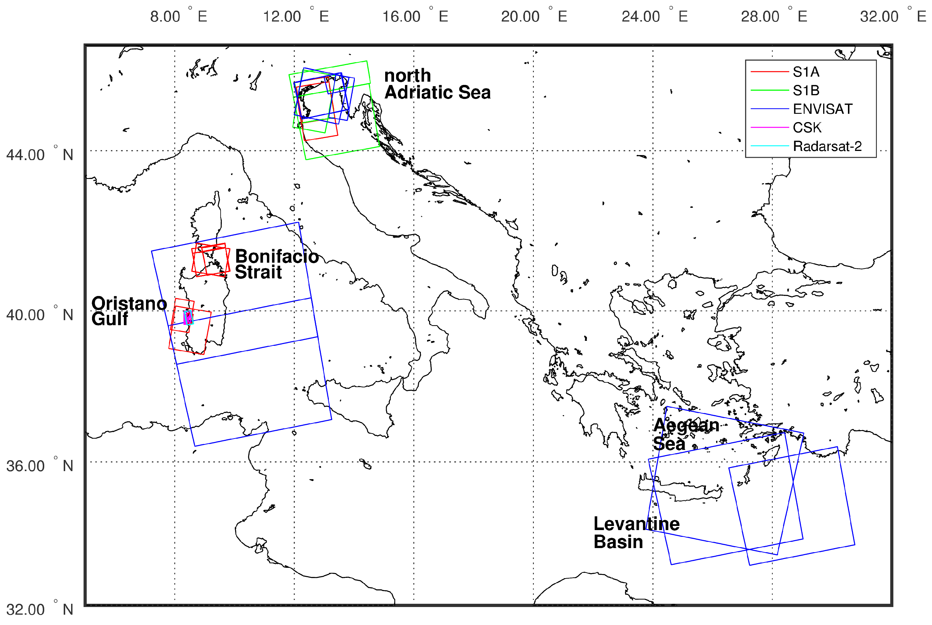
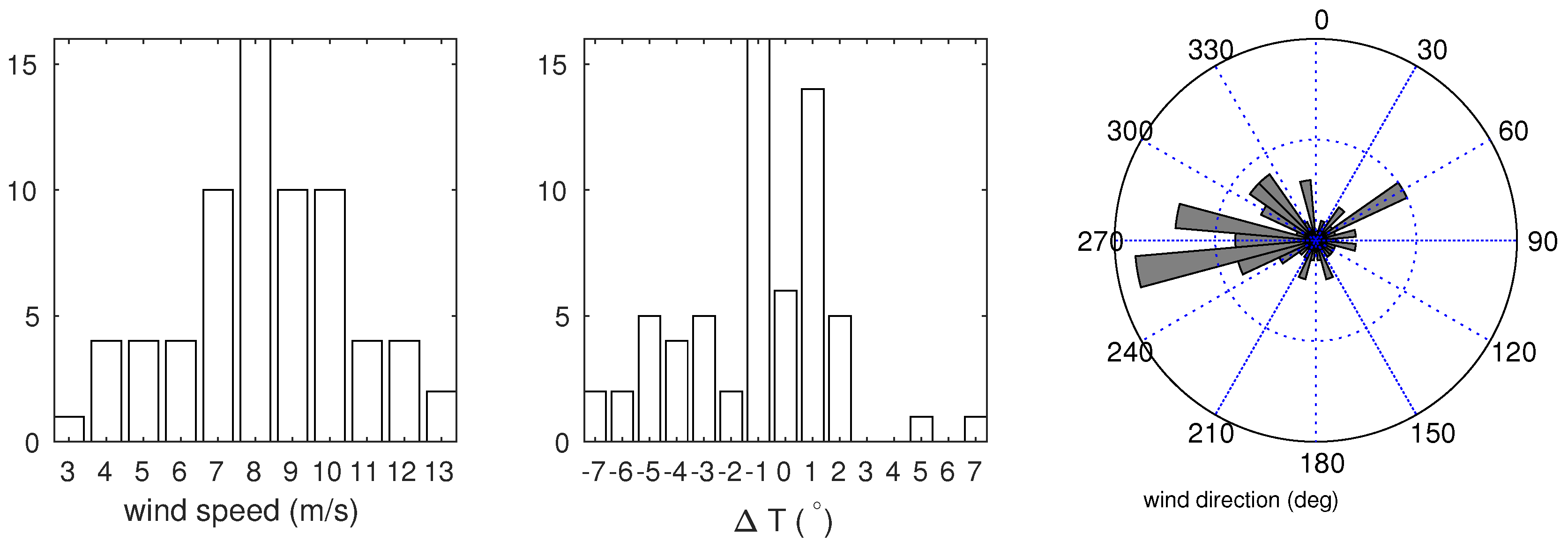
The images have been selected essentially in three coastal areas of the Mediterranean Sea (Figure 1), i.e., the northern Adriatic Sea, the Bonifacio Strait and the Oristano Gulf, according to the availability of the in situ data and the occurrence of moderate to strong wind conditions. Few images in the Levantine Basin have also been considered. They represent a large variety of possible geophysical conditions in these areas, as shown in Figure 2, which reports the statistical distributions of the wind speed, air-sea temperature difference and wind direction from the analysis fields of the European Centre for Medium-range Weather Forecasts (ECMWF) model related to the SAR images used in this work. The big deal of images has winds from 7 m/s to 10 m/s, but about ten have winds less than 6 m/s and greater than 10 m/s. The stability conditions present at the SAR overpasses were essentially neutral () with, however, a consistent number of images taken under unstable air-sea conditions. Finally, the wind direction distribution reflects that of the Mediterranean Sea, where the most probable winds come from the western quadrants [2,25].
Among them, 26 refer to the Bonifacio Strait, 20 to the Oristano Gulf where wind in situ data are available [26,27] and 11 to the northern Adriatic Sea.
The Bonifacio Strait, dividing Sardinia from Corsica islands, is mainly subjected to northwesterly winds which are often funnelled by the strait producing high winds in its eastern part [28,29]; the Gulf of Oristano is a semi-enclosed bay located along the western coast of Sardinia island (Western Mediterranean Sea), mainly subject to winds from the northwest (mistral, ≈43%) and from the southeast (Sirocco, ≈18%), according to the statistics obtained from almost 16 years of scatterometer wind data (2000–2015) [26]; the strongest winds in the northern Adriatic Sea are the northeasterly Bora and the southeasterly Sirocco, occurring mainly in Autumn and Winter, the former classified as an orographic wind [30], the latter often associated with a low pressure centred in the Tyrrhenian Sea or in the Gulf of Genoa, producing the well known storm surges in the city of Venice.
3. The Method to Extract the Wind Direction from SAR
The methods used in this work to estimate the wind directions over the sea area by SAR refines the technique described in [13,14] by using a full 2D-CWT. This method is applied to a SAR image to obtain the wavelet spectrum, which is the map of energy as a function of angle (from –90 to 90 degrees, which is the fourth and the first quadrant of the Cartesian coordinate system) and scales chosen in the range between 200 m to 2500 m. The choice of scales length roughly corresponds to the wind frequency range between and Hz, where the small scale maximum of the wind spectra lies (see [10], p. 85). The scales and angles of the maximum wavelet spectrum are then selected and used to reconstruct the SAR image, which will contain only the spatial features at those scales and angles, i.e., the features of the wind imprint of the sea surface, typically backscatter cells elongated in the wind direction. The reconstructed image is then used to make evident the backscatter cells related to the wind, from which the aliased wind direction is evaluated from the direction of the cells’ major axis.
3.1. The 2D-CWT
In the following, to briefly introduce the 2D-CWT, we follow the formalism of [31,32], to which the interested reader is addressed.
The Two-Dimensional Continuous Wavelet Transform S of a two-dimensional function (an image) is a local transform with respect to the mother wavelet depending on the parameters , the displacement, a, the dilation or scale, and , the rotation, obtained by the scalar product of s and , i.e.,
where the asterisk denotes complex conjugation. is a constant satisfying the admissibility condition and is the Fourier transform of .
Since we need a directional and thus anisotropic mother wavelet, we have used in this work the 2D Morlet wavelet
where and 1 is the anisotropy parameter.
The Morlet mother wavelet has the advantage, with respect to other anisotropic mother wavelets like, for instance, the Cauchy, to have a definite relationship between dilation scales and wave numbers: this permits defining the scales length on a geophysical basis and to convert them to dimensionless dilation scales for the computation.
The angles considered are from 0 to at steps of . Therefore, for each couple of and a, the wavelet coefficient is obtained: is related to the local energy of the original image.
Among the possible representations of the four variables wavelet transform (Equation (1)), there is the relative scale-angle energy density [32],
where is the scale-angle energy density given by
As in [32], … Whereas gives the distribution of energy at different scales and directions, gives the relative distribution at different directions at a particular scale with respect to the total energy at that scale…, revealing more efficiently the scale-space anisotropic behaviour of the signal (the SAR image in our case).
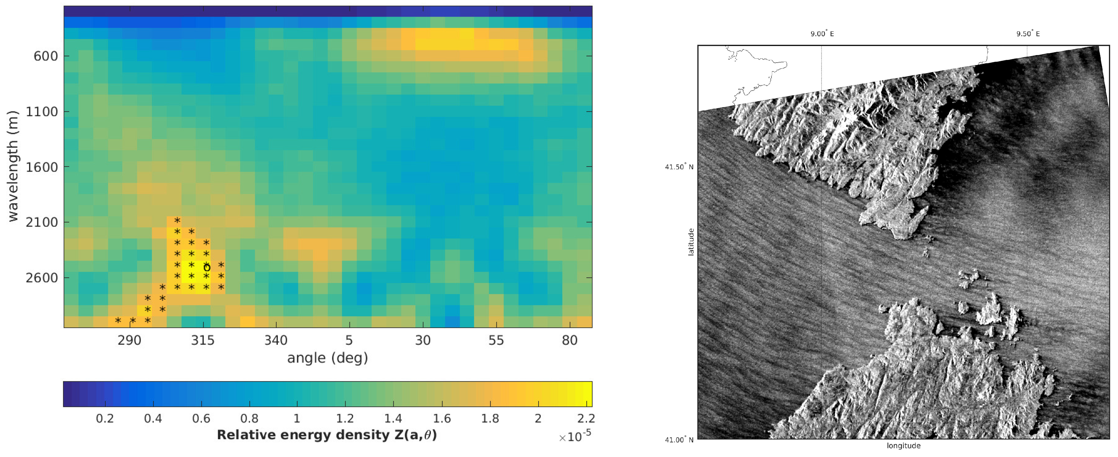
Since we are interested in identifying the directions of the most energetic backscatter structures, we have used the relative scale-angle energy density (Equation (3)) to find and select the scales and angles to reconstruct the SAR image. The resulting map of may be very different according to the geophysical phenomena imaged, i.e., ocean gravity waves, swell, atmospheric gravity waves, katabatic winds and so on. In general, all the geophysical phenomena with scale lengths inside the range of scales chosen for the 2D-CWT analysis appear in . An example is provided in Figure 3, which reports the relative scale-angle energy density (left panel) of the Sentinel-1A SAR image shown in the right panel. The energy density map, reported as a function of angles expressed in degree with respect to the geographic north (abscissae) and the scales in meters (ordinates) used in the 2D-CWT analysis, shows several relative maxima: the larger one, falling around 315 and 2600 m, accounts for the presence of the wind streaks visible in the western part of the image. The second one, falling at and 600 m, probably accounts for the sea wave fronts roughly perpendicular to the wind direction.
However, the method does not depend on the presence of wind rolls but on the backscatter structures at spatial scales smaller than them. As emphasised in [5], the wind rolls are organized as pearls on a string, and these pearls are those detected by the 2D-CWT method. This implies that the method is working well also when the wind rolls are not present, as in many SAR images analysed in this work.
3.2. Choice of the Scales and Angles and Image Reconstruction
Once the relative scale-angle energy density is obtained, we have to select the scales a and angles relative to the wind structures, with the aim of reconstructing the SAR images with only these scales/angles, in order to make evident the shape and the layout of these structures. This is accomplished taking the scale and angles exceeding the value of the 95% quantile of , with the constraint that their location must form a spatially connected ensemble.
The sum of the wavelet coefficients at the scales a and angles selected gives the reconstructed image which, after a clipping procedure, makes evident the structures with the highest energy. The clipping is done as
where is the local standard deviation computed in a sub-area of size corresponding to the maximum scale selected and centred on . The left panel of Figure 4 reports resulting from the analysis of the image shown in the right panel of Figure 3. It provides the shape of the most energetic structures related to the wind (wind cells), resulting in being broadly elliptic with the major axis aligned to the wind direction. Note the different cells’ density in the western and eastern parts of the strait: as the wind is from the northwest, the eastern part of the strait is shielded by the islands. Thus, the wind is lower and the cells less developed. This is a clear indication that the density and shape of the wind cells are dependent on the wind strength.
The aliased wind directions, obtained from the major axis orientation of the wind cells, are reported in the right panel of Figure 4. The spatial resolution of the wind cells is not regular, i.e., the backscatter cells linked to the wind are detected where they are located and not according to an a priori fixed spatial resolution. Hence, it is possible only to provide an effective spatial resolution of the resulting fields from the number of wind directions derived by the 2D-CWT. In the case of the image from Figure 4, this is of ≈3.2 km.
Furthermore, not only the aliased wind direction can be extracted from the results of the 2D-CWT analysis, but also the size of the backscatter cells and their spatial density. This information can be used to investigate their dependence on the wind speed, atmospheric stability and fetch, gaining new insights about the spatial structure of the marine atmospheric boundary layer.
3.3. Operational Methodology
The images have been under sampled to ≈100 m prior to being analysed by the 2D-CWT, in order to avoid the signal of the ocean gravity waves, if present, entering into the analysis. This signal due to waves is usually more energetic than the signal of the wind. The 2D-CWT analysis is performed on the SAR images in dB and the relative scale-angle energy density obtained. The scales and angles of the energy spectrum around its maximum value exceeding the 0.95 quantile are then selected and used to get the clipped image reconstruction . From the structures evidenced in , the aliased direction is computed. De-aliasing is performed according to the ECMWF mean wind direction over the area.
4. Results
For all areas, the results are provided in terms of comparison between the SAR derived and the ECMWF wind directions averaged over the area imaged by SAR. The ECMWF data are the analysis winds supplied every six hours (12:00 a.m., 6:00 a.m. GMT…), temporally interpolated to the satellite pass time. In this comparison, we have to remind readers that in coastal areas the wind directions from global models are often only roughly representative of the actual wind directions, essentially due to the models’ real space resolution [2,27].
When available, satellite scatterometer wind data, i.e., the NASA QuikSCAT [33] and the EUMETSAT Advanced SCATterometer (ASCAT) a and b [34] at 12.5 km spatial grid, have also been used for comparisons. Only the scatterometer data falling in the time window ± 2 h from the SAR pass time have been selected. We have to point out, however, that comparisons with scatterometer data refer to offshore areas, as scatterometers do not provide winds closer than ≈ 20 km from coast.
The SAR directions in the Oristano Gulf are compared also with the available in situ data, collected from 2014 to 2016 in the framework of the RITMARE Italian project [26,35].
In addition to the scatter plots, also the SAR vs. ECMWF, in situ and scatterometer direction statistics is reported in terms of the bias , the Root Mean Square deviation and the linear correlation . has been computed following [36], and following [37]. ranges from 0 (no correlation) to 2 (perfect correlation).
4.1. SAR Derived versus ECMWF Wind Directions
For each image, the ECMWF wind direction data falling in the image have been selected and averaged and then compared with the SAR derived wind direction average. Due to the different spatial resolution of these data, it does not make sense to compare the data point to point.
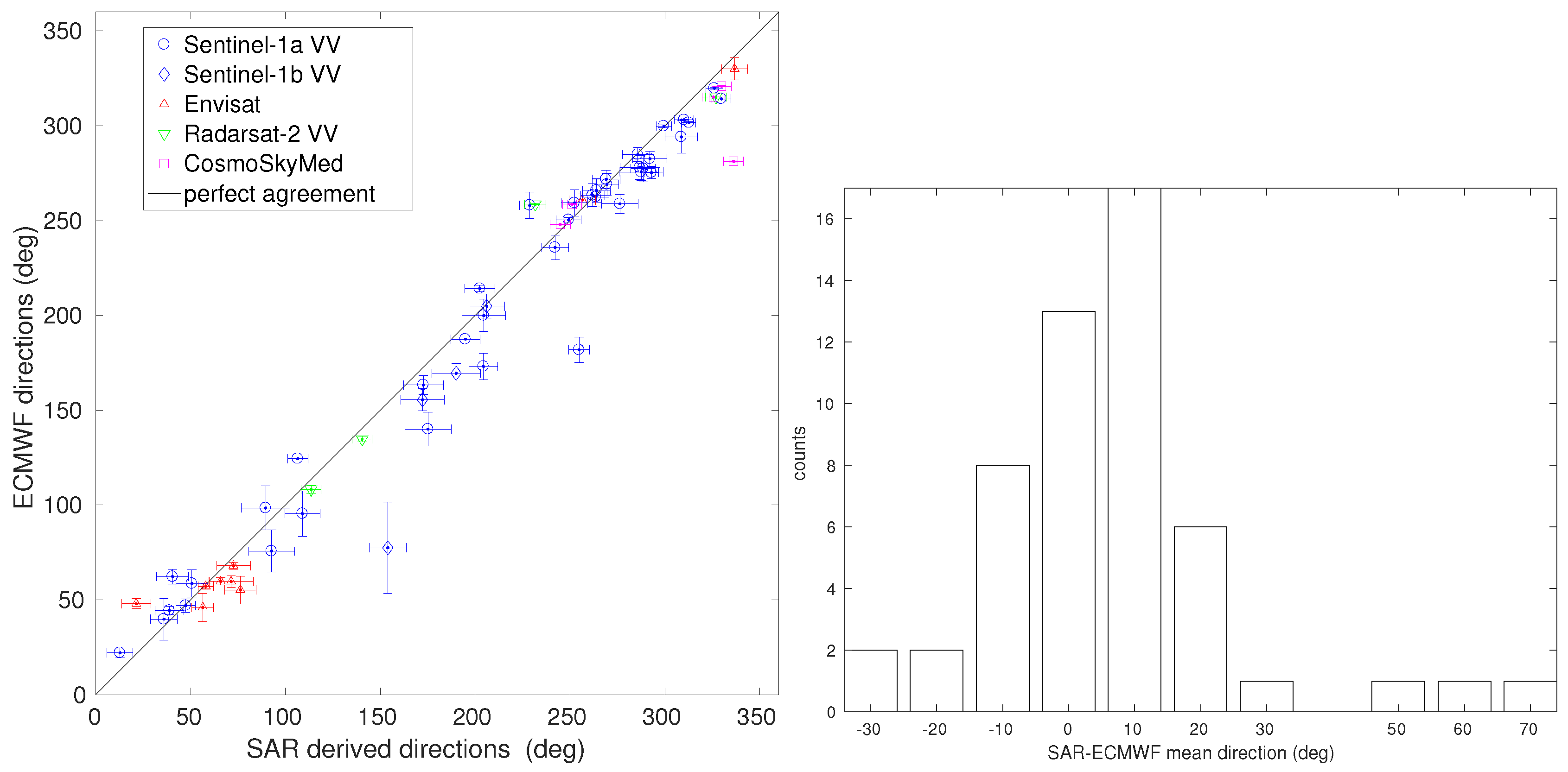
The left panel of Figure 5 reports the scatter plot between the SAR and ECMWF mean wind directions along with their standard deviation. Note that ECMWF data sometimes have a low standard deviation due to a small amount of data falling into the area imaged, a number one order of magnitude smaller (20 in average per image) than that of the SAR winds. However, in general, the wind direction variability is larger from the SAR than from the ECMWF data (14 and 9, respectively), confirming the results obtained in [27] using a limited area atmospheric model. In that paper, it was shown that the SAR directions variability is close to that derived from in situ data.
The comparison is very satisfactory, the correlation is high (), and the mean bias is and .
A more detailed analysis of the results is provided by the distribution of the SAR minus ECMWF wind directions provided in the right panel of Figure 5: for 83% of cases, the difference is , for 92. Only in three cases (5%) is the direction difference greater than 50.
4.2. SAR Derived versus In Situ and Scatterometer Wind Directions
The in situ winds have been derived from the network of five three-axial anemometers installed on the Oristano Gulf coast, a few meters from the sea [26]. They measured the three components of the wind continuously at 1 Hz sampling.
The comparison between time and space dependent data is never an easy task. For those between the SAR derived and the in situ directions, a fixed spatial window = 4000 m has been chosen, roughly corresponding to one fourth of the Oristano Gulf size, while a varying temporal window has been derived according to the wind speed , i.e., . This time window has been used to compute the mean values of the measured wind directions centred at the SAR pass time; the mean SAR directions have been obtained averaging the wind direction falling in the areas of radius centred at each in situ site. The mean values of the in situ wind directions have been obtained over a time window positioned before or after the SAR pass time depending if the wind blew from sea to land or vice-versa. The resulting comparison, shown in the left panel of Figure 6, is satisfactory, with and and . Here, we have to note that the in situ winds were measured at the sea–land interface, while the SAR ones were measured over the sea. Therefore, some discrepancies may arise from the different nature of the data.
As noted before, scatterometer winds never cover the entire area images by SAR because they do not sense the coastal areas. The mean values of SAR wind directions used here are therefore a sub-set of those retrieved, whose area overlaps that of the scatterometer data. As for the ECMWF data, the mean values in the overlapping areas have been compared. The right panel of Figure 6 reports the SAR versus scatterometer wind direction averaged in the overlapped area along with their standard deviation. The scatterometer mean values are derived from few data (20 in average per image), while the SAR winds are one order of magnitude larger. The statistics provides and and .
5. Discussion
The 2D-CWT method used to estimate the wind direction from SAR images provides satisfactory results, both in areas few kilometres from coast like the Gulf of Oristano and offshore. It is reliable as it produces good estimates no matter which is the satellite SAR, hence which is the original pixel size and the SAR viewing parameters. Furthermore, even if only five X-band images have been used in this work, it seems that the SAR frequency does not influence the 2D-CWT results. The results are good despite the different nature of the wind data to which the SAR wind directions have been compared.
However, there are few cases where the wind directions estimated by the 2D-CWT seem to differ significantly from the external wind directions such as those from atmospheric models and satellite scatterometer. Let us analyse a case of them, that of a Sentinel-1B image over the northern Adriatic Sea, reported in the top left panel of Figure 7. The SAR image is characterized by two different backscatter signatures areas, divided by a front-like roughly starting at 45 N, 12.5 E. In the northern part, large signatures of atmospheric gravity waves, often associated with the northeasterly wind, are visible, while the southern part the classic wind rolls are present. The SAR wind directions obtained by the 2D-CWT are reported in the top right panel. For this case, the comparison with the ECMWF produces the isolated point at about 140 and 80 (see the left panel of Figure 5). The meteorological situation present at the SAR pass time, typical of this area, is shown in bottom left panel of Figure 7, which reports the wind field from ECMWF temporally interpolated at the SAR pass time: a strong southeasterly wind is blowing in the southern part of the area, while a northeasterly in its northern one. There are two wind systems coexisting, the Sirocco in the southern and the Bora in the northern part of the images area. Also the ASCAT winds taken two hours later than the SAR pass time (7.09 p.m. GMT), shown in the bottom right panel of Figure 7, report this situation, however without showing a clear discontinuity. The SAR wind directions do not follow the sharp bending of the wind, shown in the ECMWF field. In the present formulation, the 2D-CWT is unable to provide accurate wind directions of the sharp bending fields: this is a rather general shortcoming of this methodology, which must be solved with further work.
The determination of the wind direction from SAR, hence of the wind field if the radar backscatter-wind speed models are available, is important in the coastal areas, where the short-term prediction of the main hydrodynamics such as the sea water temperatures and salinity, water currents, wind wave height and so on by means of numerical modelling techniques is strongly sensitive to the spatial and temporal variability of the wind. The SAR is able to provide the spatial variability of the wind over the sea in a unique way. In [27], it was shown that even the high resolution regional models are unable to provide details of the wind spatial layout similar to those provided by SAR, and that the spatial variability of the SAR winds is compatible with that derived from the in situ data.
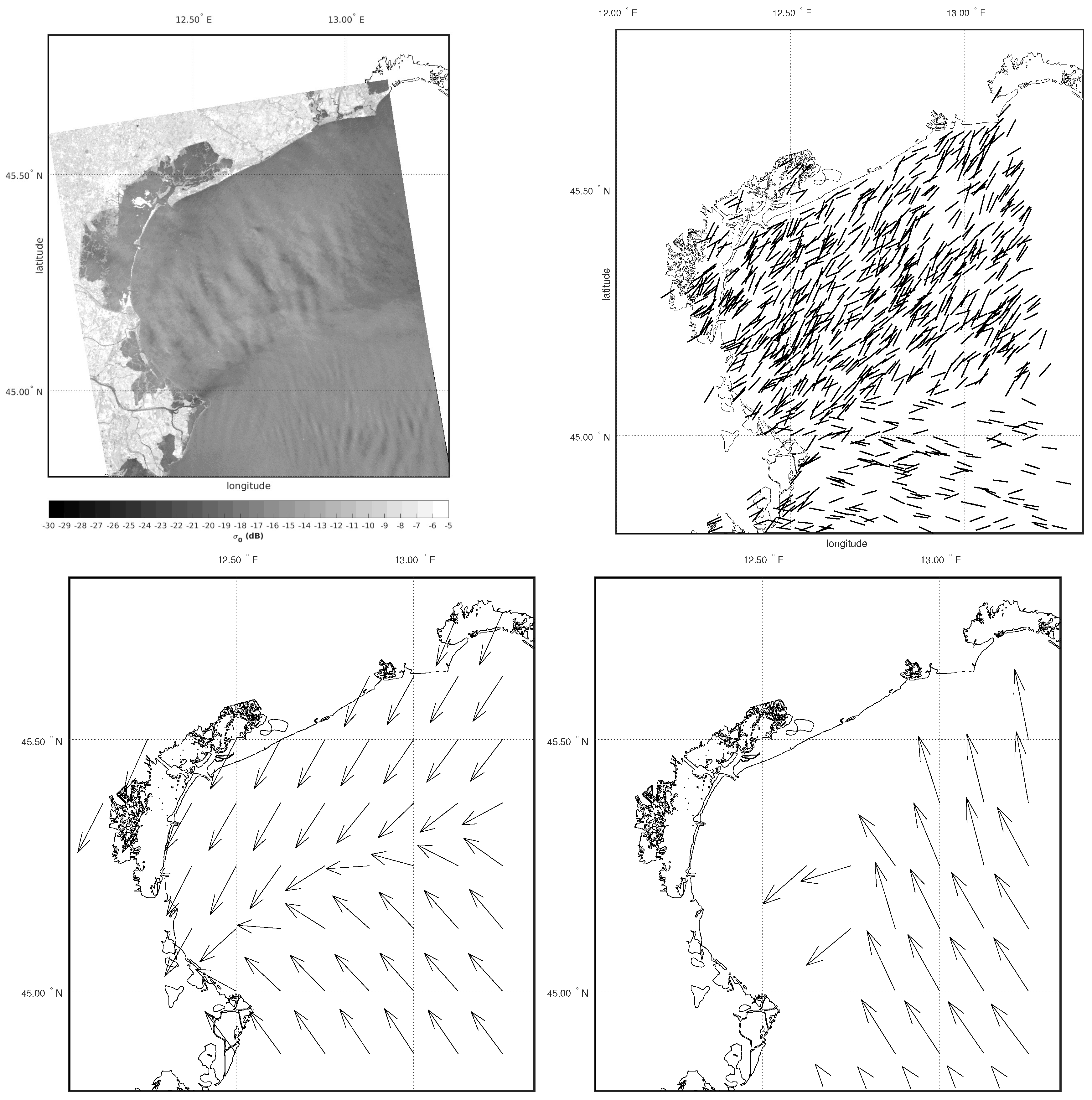
To illustrate these capabilities, an example of northeasterly wind in the northern Adriatic Sea as described by ECMWF and by SAR directions is shown in Figure 8, which reports the SAR derived directions overlapped by those from ECMWF (bold arrows) on the 6 February 2017 at 4:58 p.m. GMT.
It is easy to appreciate the quality of details provided by the SAR directions in contrast with the smooth field provided by ECMWF. In particular, the wind direction estimates very close to the coast and also inside the Venice lagoon are the added value brought by the SAR winds.
The last comment concerns the nature of the data used for comparisons with the SAR wind directions. The atmospheric model data are known to have problems in description of coastal winds [2,38], essentially because of their real spatial resolution. In particular, those used in this paper, available at six-hour intervals, have been temporally interpolated at the SAR pass time, a fact that may introduce errors in fast changing winds. This remark applies also to scatterometer data, taken ±2 h from the SAR pass time. The in situ data were measured very close to the sea but over land; therefore, they cannot be fully representative of the winds over the sea.
The wind directions at the SAR pass time over the sea are virtually unknown, and the figures provided by SAR are highly valuable, even not properly validated. Ad hoc campaigns would be necessary to validate the 2D-CWT method proposed in this paper.
6. Conclusions
The 2D-CWT method is one of the few techniques able to evaluate the wind directions from SAR images without any external information; an external information is needed only to de-alias the directions, but it does not influence either their layout or their value. Its performance does not depend from the satellite and seems also not to be sensitive from the SAR radar frequency. It may depend, however, from the size of the area imaged, as in large areas the wind directions are less spatially uniform than the small ones.
This technique permits evaluating the wind direction, necessary to invert the vs. wind speed relationship, directly from the radar signatures present in the image, without any external wind direction information. This is particularly important in coastal areas, where the wind directions from atmospheric models, usually used to this aim, may be not fully reliable, as discussed in [2]. Therefore, the use of model wind directions to derive the SAR wind field is highly inadvisable in coastal areas.
The wind field determination from SAR images cannot prescind from a trusted methodology to estimate the wind direction. The results of this work indicate that the 2D-CWT technique is reliable enough to be a necessary step toward the determination of the wind field. This can open the possibility of using the SAR derived wind fields to study the characteristics of the marine atmospheric boundary layer, as the spectral shape of the wind under different geophysical situations, the spatial distribution and size of the backscatter/wind cells under different stability and wind regimes, the spatial variability of the wind speed.
Acknowledgments
This work has been partially supported by the project RITMARE (www.ritmare.it) funded by the Italian Ministry of University and Research. The COSMO-SkyMed and Radarsat-2 SAR images have been obtained in the framework of the COSMO-SkyMed/RADARSAT-2 Initiative of the Italian Space Agency and the Canadian Space Agency Ocean wind fields from C and X-band SAR in the coastal areas, Proposal id 2868/5224. The Envisat ASAR images where obtained from ESA Eoli-SA archive. The Sentinel-1 images have been downloaded from the ESA Sentinels Scientific Data Hub (https://scihub.copernicus.eu/). The ECMWF fields have been obtained thanks to the authorization from the Aereonautica Militare of Italy. The scatterometer data have been downloaded from the NASA Physical Oceanography Distributed Active Archive Center at the Jet Propulsion Laboratory/California Institute of Technology. The author wishes to thank the Referees for their effort to review the paper.
Conflicts of Interest
The author declares no conflict of interest.
References
- Accadia, C.; Zecchetto, S.; Lavagnini, A.; Speranza, A. Comparison of 10-m Wind Forecasts from a Regional Area Model and QuikSCAT Scatterometer Wind Observations over the Mediterranean Sea. Mon. Weather Rev. 2007, 135, 1946–1960. [Google Scholar] [CrossRef]
- Zecchetto, S.; Accadia, C. Diagnostics of T1279 ECMWF analysis winds in the Mediterranean Basin by comparison with ASCAT 12.5 km winds. Q. J. R. Meteorol. Soc. 2014, 140, 2506–2514. [Google Scholar] [CrossRef]
- Gerling, T. Structure of the surface wind field from Seasat SAR. J. Geophys. Res. 1986, 91, 2308–2320. [Google Scholar] [CrossRef]
- Thompson, T.W.; Liu, W.T.; Weissman, D.E. Synthetic Aperture Radar observation of ocean roughness from rolls in an unstable marine boundary layer. Geophys. Res. Lett. 1983, 10, 1172–1175. [Google Scholar] [CrossRef]
- Etling, D.; Brown, R.A. Roll vortices in the planetary boundary layer: A review. Bound. Layer Meteorol. 1993, 65, 215–248. [Google Scholar] [CrossRef]
- Tsai, W.T. On the formation of streaks on wind-driven water surfaces. Geophys. Res. Lett. 2001, 28, 3959–3962. [Google Scholar] [CrossRef]
- Zhao, Y.; Li, X.M.; Sha, J. Sea surface wind streaks in spaceborne synthetic aperture radar imagery. J. Geophys. Res. Oceans 2016, 121, 6731–6741. [Google Scholar] [CrossRef]
- Thomson, R.E.; Vachon, P.W.; Borstad, G.A. Airborne synthetic aperture radar imagery of atmospheric gravity waves. J. Geophys. Res. 1992, 97, 14249–14257. [Google Scholar] [CrossRef]
- Pierson, W.J. The measurement of the synoptic scale wind over the ocean. J. Geophys. Res 1983, 88, 1683–1708. [Google Scholar] [CrossRef]
- Panofsky, H.A.; Dutton, J.A. Atmospheric Turbulence; John Wiles & Sons: Hoboken, NJ, USA, 1984. [Google Scholar]
- Antoine, J.P.; Duval-Destin, M.; Murenzi, R.; Piette, B. Image analysis with 2D wavelet transfor: Detection of position, orientation and visual contrast of simple objects. In Wavelets and Applications, Proceedings Marseille 1989; Meyer, Y., Ed.; Springer and Masson: Berlin, Germany; Paris, France, 1991; pp. 144–159. [Google Scholar]
- Antoine, J.P.; Carrette, P.; Murenzi, R.; Piette, B. Image analysis with two-dimensional continuous wavelet transform. Signal Process. 1993, 31, 241–272. [Google Scholar] [CrossRef]
- Zecchetto, S.; De Biasio, F. On shape, orientation and structure of atmosheric cells inside wind rolls in two SAR images. IEEE Trans. Geosci. Remote Sens. 2002, 40, 2257–2262. [Google Scholar] [CrossRef]
- Zecchetto, S.; De Biasio, F. A Wavelet Based Technique for Sea Wind Extraction from SAR Images. IEEE Trans. Geosci. Remote Sens. 2008, 46, 2983–2989. [Google Scholar] [CrossRef]
- Vachon, P.; Dobson, F. Wind Retrieval from Radarsat SAR Images: Selection of a Suitable C-Band HH Polarization Wind Retrieval Model. Can. J. Remote Sens. 2000, 24, 306–313. [Google Scholar] [CrossRef]
- Du, Y.; Vachon, P.W.; Wolfe, J. Wind direction estimation from SAR images of the ocean using wavelet analysis. Can. J. Remote Sens. 2002, 28, 498–509. [Google Scholar] [CrossRef]
- Horstmann, J.; Koch, W.; Lehner, S. High resolution wind fields retrieved from SAR in comparison to numerical models. In Proceedings of the IEEE International Geoscience and Remote Sensing Symposium, Toronto, ON, Canada, 24–28 June 2002. [Google Scholar]
- Staples, G.; Mendoza, A. The Use of RADARSAT-1 SAR Data for Operational Wind Field Retrieval. In Proceedings of the IEEE International Geoscience and Remote Sensing Symposium, Toronto, ON, Canada, 24–28 June 2002. [Google Scholar]
- Koch, W. Directional Analysis of SAR Images Aiming at Wind Direction. IEEE Trans. Geosci. Remote Sens. 2004, 42, 702–710. [Google Scholar] [CrossRef]
- Zhou, L.; Zheng, G.; Li, X.; Yang, J.; Ren, L.; Chen, P.; Zhang, H.; Lou, X. An improved local gradient method for sea surface wind direction retrieval from SAR Imagery. Remote Sens. 2017, 9, 671. [Google Scholar] [CrossRef]
- Agenzia Spaziale Italiana (ASI). COSMO-SkyMed System Description & User Guide; Agenzia Spaziale Italiana: Rome, Italy, 2007. [Google Scholar]
- MacDonald, Dettwiler and Associates Ltd. Radarsat-2 Product Description; MacDonald, Dettwiler and Associates Ltd.: Richmond, BC, Canada, 2015. [Google Scholar]
- European Space Agency. ASAR Product Handbook; Technical Report; European Space Agency: Paris, France, 2007. [Google Scholar]
- European Space Agency. Sentinel-1 User Handbook. ESA Standard Document. 1 September 2013. Available online: https://sentinel.esa.int/ (accessed on 1 September 2013).
- Meteorological Office. General Meteorology. In Weather in the Mediterranean; Her Majesty’s Stationary Office: London, UK, 1962; Volume 1. [Google Scholar]
- Zecchetto, S.; della Valle, A.; De Biasio, F.; Quattrocchi, G.; Cadau, E.; Cucco, A. The wind measuring system in the Gulf of Oristano as support to the regional scale oceanographic modeling. J. Oper. Oceanogr. 2016, 9, 144–154. [Google Scholar] [CrossRef]
- Zecchetto, S.; De Biasio, F.; della Valle, A.; Quattrocchi, G.; Cadau, E.; Cucco, A. Wind Fields from C and X band SAR images at VV polarization in coastal area (Gulf of Oristano, Italy). IEEE J. Sel. Top. Appl. Earth Obs. Remote Sens. 2016, 9, 2643–2650. [Google Scholar] [CrossRef]
- Zecchetto, S.; Cappa, C. The spatial structure of the Mediterranean Sea winds revealed by ERS-1 scatterometer. Int. J. Remote Sens. 2001, 22, 45–70. [Google Scholar] [CrossRef]
- Zecchetto, S.; De Biasio, F. Sea surface winds over the Mediterranean Basin from satellite data (2000–2004): Meso- and local-scale features on annual and seasonal timescales. J. Appl. Meteorol. Climatol. 2007, 46, 814–827. [Google Scholar] [CrossRef]
- Atkinson, B.W. Meso-Scale Atmospheric Circulation; Academic Press: London, UK, 1989. [Google Scholar]
- Antoine, J.P.; Murenzi, R. Two-Dimensional directional wavelets and the scale-angle representation. Signal Process. 1996, 52, 259–281. [Google Scholar] [CrossRef]
- Antoine, J.P.; Murenzi, R.; Vandergheynst, P.; Twareque Ali, S. Two-Dimensional Wavelets and Their Relatives; Cambridge University Press: Cambridge, UK, 2004. [Google Scholar]
- Jet Propulsion Laboratory. QuikSCAT Level 2B Version 3 Guide Document; Technical Report v1; California Institute of Technology: Pasadena, CA, USA, 2013.
- OSI-SAF-EARS. In ASCAT Wind Product User Manual (Ver. 1.14); Technical Report SAF/OSI/CDOP/KNMI/TEC/MA/126; Eumetsat: Darmstadt, Germany, 2016; Available online: http://www.knmi.nl/scatterometer/publications/pdf/ (accessed on 1 December 2017).
- RITMARE. Italian Flag Project of the National Program of Research Funded by the University and Research Ministry of Italy, 2012–2016. Available online: http://www.ritmare.it (accessed on 1 December 2017).
- Yamartino, A. A comparison of several single-pass estimators of the standard deviation of wind direction. J. Clim. Appl. Meteorol. 1984, 23, 1362–1366. [Google Scholar] [CrossRef]
- Crosby, D.S.; Breaker, L.S.; Gemill, W.H. A proposed definition for vector correlation in geophysics: Theory and application. J. Atmos. Ocean. Technol. 1993, 10, 355–367. [Google Scholar] [CrossRef]
- Liu, T.W.; Tang, W.; Polito, P.S. NASA scatterometer provides global ocean-surface wind fields with more structures than numerical weather prediction. Geophys. Res. Lett. 1998, 25, 761–764. [Google Scholar] [CrossRef]
Figure 1.
The frames of the Synthetic Aperture Radar images used in this work in the Mediterranean Sea. S1A/B: Sentinel-1 A/B; Envisat: ASAR WS; CSK: COSMO-SkyMed; Radarsat-2: Scansar Narrow.
Figure 1.
The frames of the Synthetic Aperture Radar images used in this work in the Mediterranean Sea. S1A/B: Sentinel-1 A/B; Envisat: ASAR WS; CSK: COSMO-SkyMed; Radarsat-2: Scansar Narrow.

Figure 2.
Geophysical conditions in the areas imaged by the SARs used in this work according to the analysis data of the European Centre for Medium-range Weather Forecasts (ECMWF) model. Left panel: wind speed distribution. Middle panel: air-sea temperature difference distribution. Right panel: wind direction distribution.

Figure 3.
The relative scale-angle energy density spectrum (left panel) derived from the Sentinel-1A SAR image of the 3 February 2016 (S1A_IW_GRDH_1SDV_20160203T172129_20160203T172154_009785_00E4F4_AE4D) (right panel) of the Bonifacio Strait (see Figure 1). has been plotted as a function of the angles expressed in degree respect to the geographic north (abscissae) and the scales in meters (ordinates) used in the Two-Dimensional Continuous Wavelet Transform analysis. In the left panel, the stars indicate the scales and angles selected for the image reconstruction and the circle the spectrum maximum value.

Figure 4.
Results from the 2D-CWT analysis of the image shown in the right panel of Figure 3. Left panel: showing the backscatter cells related to the wind. Right panel: the aliased wind direction obtained from the orientation of the major axis of the backscatter cells showed in the left panel.
Figure 4.
Results from the 2D-CWT analysis of the image shown in the right panel of Figure 3. Left panel: showing the backscatter cells related to the wind. Right panel: the aliased wind direction obtained from the orientation of the major axis of the backscatter cells showed in the left panel.

Figure 5.
Comparison between SAR derived versus ECMWF wind directions for all the images. Left panel: scatter plot. The bars report the standard deviations. Solid line: perfect agreement. Right panel: SAR minus ECMWF wind direction difference distribution.
Figure 5.
Comparison between SAR derived versus ECMWF wind directions for all the images. Left panel: scatter plot. The bars report the standard deviations. Solid line: perfect agreement. Right panel: SAR minus ECMWF wind direction difference distribution.

Figure 6.
Comparison between SAR derived, in situ and scatterometer wind directions. Left panel: SAR versus in situ wind directions for the Oristano Gulf area. Right panel: SAR derived versus scatterometer wind directions. The bars report the standard deviations. Solid line: perfect agreement.
Figure 6.
Comparison between SAR derived, in situ and scatterometer wind directions. Left panel: SAR versus in situ wind directions for the Oristano Gulf area. Right panel: SAR derived versus scatterometer wind directions. The bars report the standard deviations. Solid line: perfect agreement.

Figure 7.
A case of discrepancy between the SAR, ECMWF and scatterometer wind directions in the northern Adriatic Sea, 5 February 2017 at 5:05 p.m. GMT. Top left panel: the Sentinel-1B SAR image S1B_IW_GRDH_1SDV_20170205T170532_20170205T170600_004168_007363_EC8E. Top right panel: SAR aliased wind direction field obtained by the 2D-CWT. Bottom left panel: ECMWF wind field interpolated on the SAR pass time. Bottom right panel: wind field at 7.09 p.m. GMT from the EUMETSAT Advanced SCATterometer-a.

Figure 8.
The SAR derived wind directions overlapped by those from ECMWF (bold arrows, not in scale) in the northern Adriatic Sea, 6 February 2017 4:58 p.m. GMT. The SAR wind directions have been obtained from the Sentinel-1A image S1A_IW_GRDH_1SDV_20170206T165804_20170206T165829_015166_018D05_344A.


Table 1.
Main characteristics of the Synthetic Aperture Radar (SAR) images used in this work.
| Satellite | CSK | RS2 | Envisat | S1A/S1B |
|---|---|---|---|---|
| Image type | Stripmap Himage | Scansar Narrow | ASAR WS | HR-GRD-IW |
| Band | X | C | C | C |
| Pixel in range (m) | 1.3 | 25 | 75 | 10 |
| Pixel in azimuth (m) | 2.1 | 25 | 75 | 10 |
| Date | 2014 to 2017 | 2014 to 2017 | 2002 to 2012 | 2014 to 2017 |
| Winter and Spring | Winter and Spring | |||
| # images processed | 5 | 4 | 9 | 43 |
COSMO-SkyMed (CSK), Radarsat-2 (RS2), Sentinel-1A,B (S1A,B).
© 2018 by the author. Licensee MDPI, Basel, Switzerland. This article is an open access article distributed under the terms and conditions of the Creative Commons Attribution (CC BY) license (http://creativecommons.org/licenses/by/4.0/).
Share and Cite
MDPI and ACS Style
Zecchetto, S. Wind Direction Extraction from SAR in Coastal Areas. Remote Sens. 2018, 10, 261. https://doi.org/10.3390/rs10020261
AMA Style
Zecchetto S. Wind Direction Extraction from SAR in Coastal Areas. Remote Sensing. 2018; 10(2):261. https://doi.org/10.3390/rs10020261
Chicago/Turabian StyleZecchetto, Stefano. 2018. "Wind Direction Extraction from SAR in Coastal Areas" Remote Sensing 10, no. 2: 261. https://doi.org/10.3390/rs10020261
Note that from the first issue of 2016, this journal uses article numbers instead of page numbers. See further details here.