Estimating Vegetation Water Content and Soil Surface Roughness Using Physical Models of L-Band Radar Scattering for Soil Moisture Retrieval


Abstract
:
1. Introduction
2. Method
- Soil surface roughness is retrieved simultaneously as soil moisture and VWC are estimated. Surface roughness is specified as constant in time, which is the key concept of the time-series retrieval method to avoid ill-conditions. In comparison, VWC and soil moisture estimates are allowed to vary temporally.
- VWC estimate modifies a ‘first guess’. The first guess is the in situ values for airborne campaign data and 16-daily MODIS-climatology for SMAP. The modification factor fi can be either static or dynamic in time. When the VWC is not expected to change in time over natural terrain, a static f formulates Equation (2).
- On the other hand, over croplands where the vegetation changes significantly with the crop growth, fi is allowed to vary dynamically. To prevent ill-conditions, regularization or limits are required. By acknowledging that plant growth is steady, VWC change is allowed to vary up to a fixed limit (1.25 times of the VWC retrieval at the previous time step during the soybean growth [27]), and up to pre-defined values for the other respective crops.
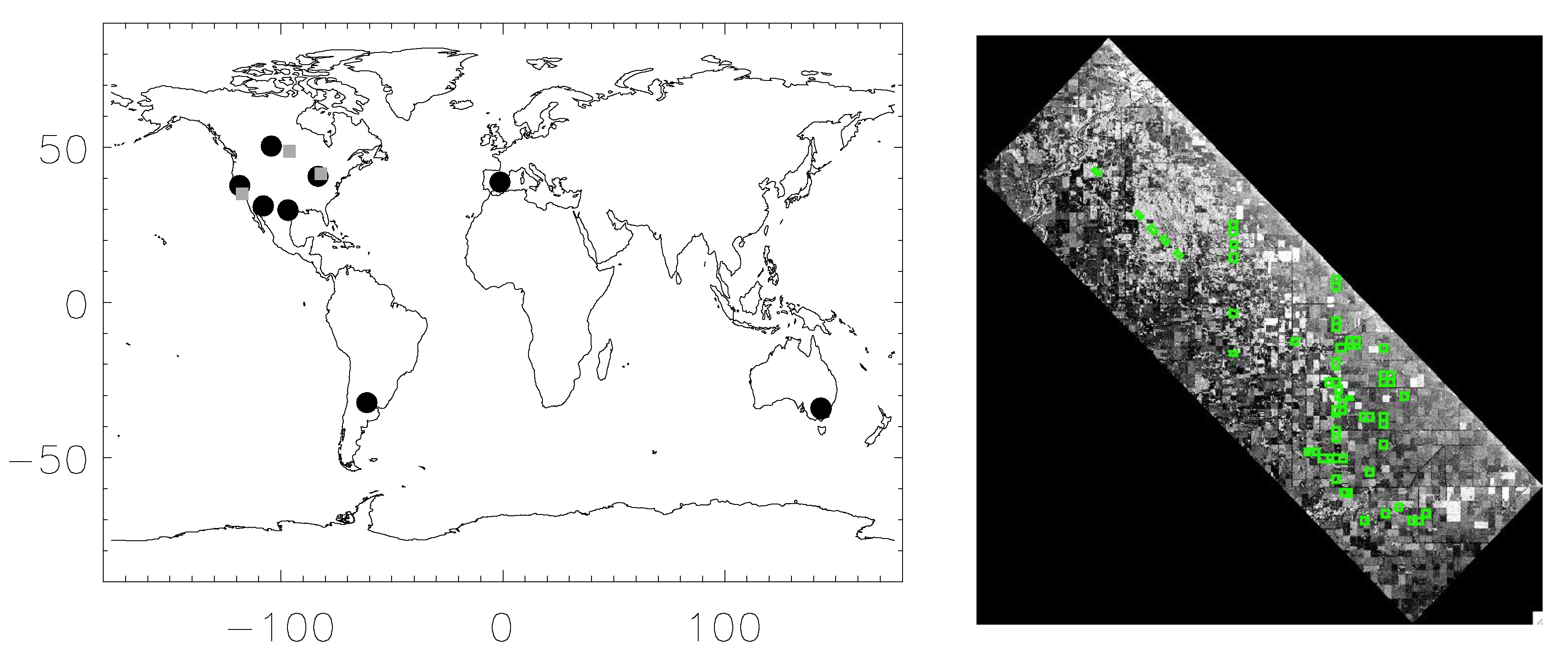
3. Data
4. Results and Discussion
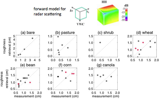
4.1. Surface Roughness Retrieval
- -
- First, we examine various properties of the retrieval for soundness. The retrieved values range from 0.5 cm to 4 cm, which are realistic within the range for isotropic surfaces. To the extent that the changes to σ0 by terrain slope within 3-km pixel are temporally static, they are corrected by the bias correction (c in Equation (2)) and the scattering may represent those from the isotropic surfaces. Considering the departure of the surface condition from the isotropic assumption, the SMAP retrievals are more likely to be an effective roughness.
- -
- Second, there is a general trend towards rougher surfaces in croplands, suggesting the impacts by farming operations on soil surfaces. The mean of the retrieved roughness is 2.6 cm (cropland) and 1.5 cm (natural terrain).
- -
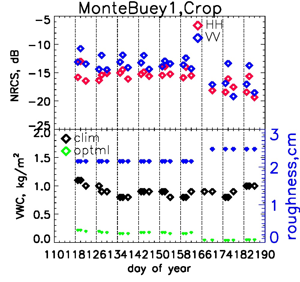
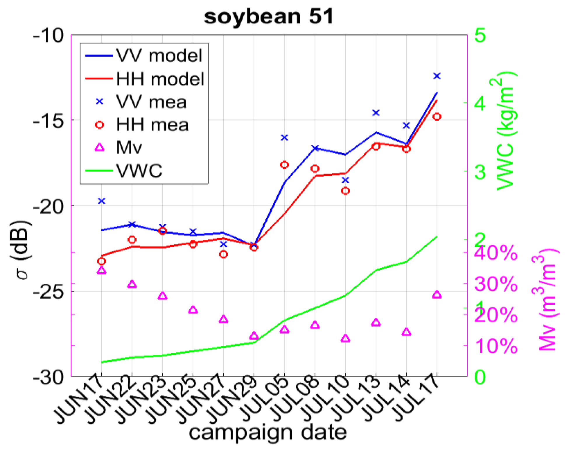
- An interesting case is found in the Monte Buey site, cropland with mostly soybeans in central Argentina. After day 160 (9 June), σ0 suddenly decreased (Figure 4). According to the ground observation, a harvest ended around day 153 with surface roughness having changed during the harvest. Additional experiments were performed: soil moisture, VWC and surface roughness were retrieved for two separate periods: before and after the harvest. After the harvest, the surface roughness increased (from 2.15 cm to 2.47 cm) and VWC is reduced (VWC factor, f, changing from 0.3 to 0.05), which are consistent with the expectation of post-harvest conditions.
4.2. VWC Retrieval
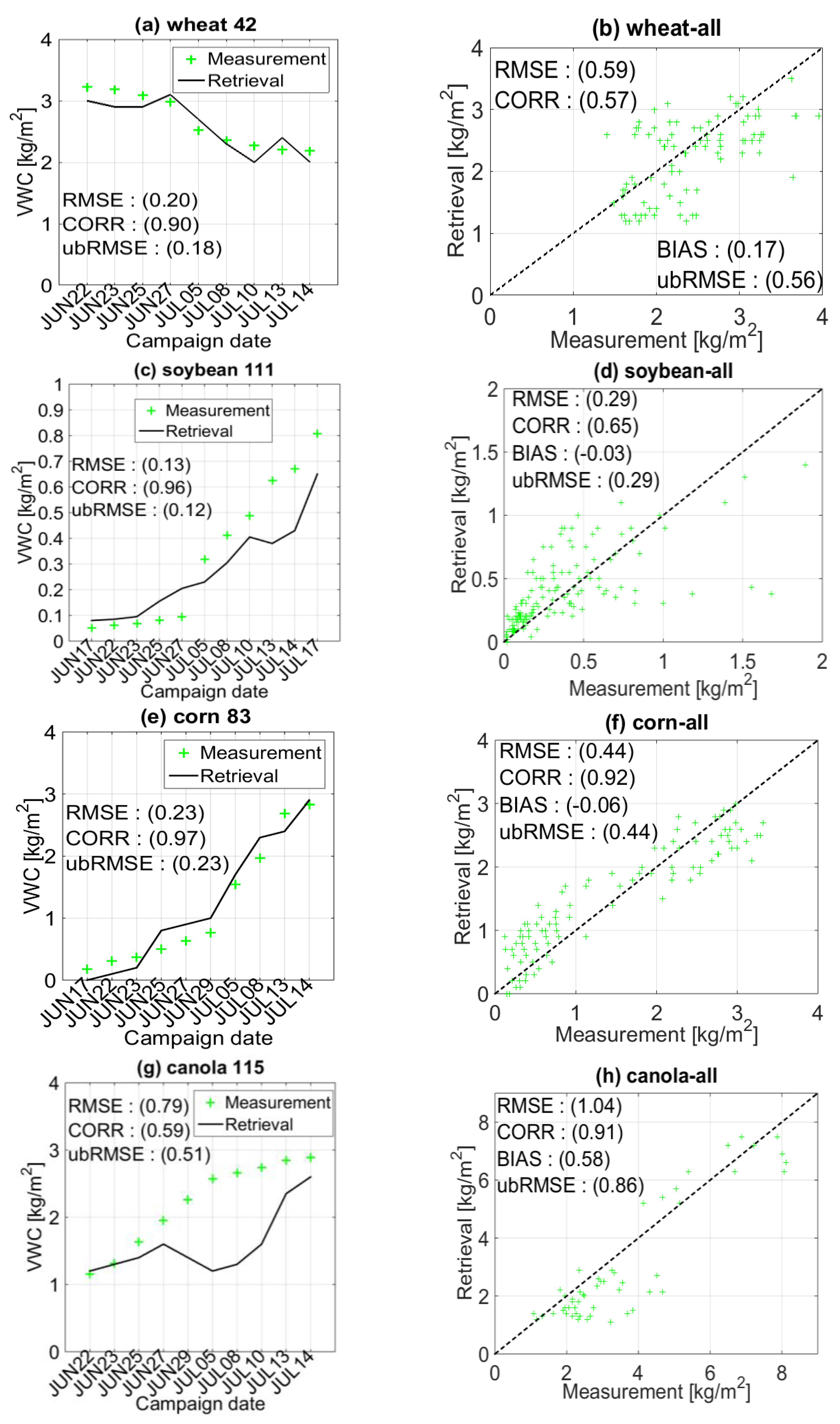
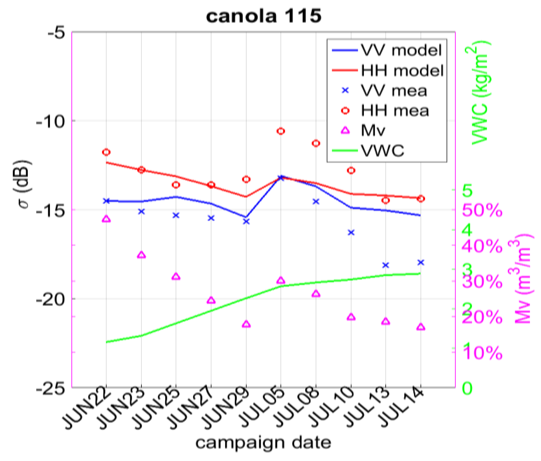
4.2.1. SMAPVEX12
4.2.2. SMAP
- -
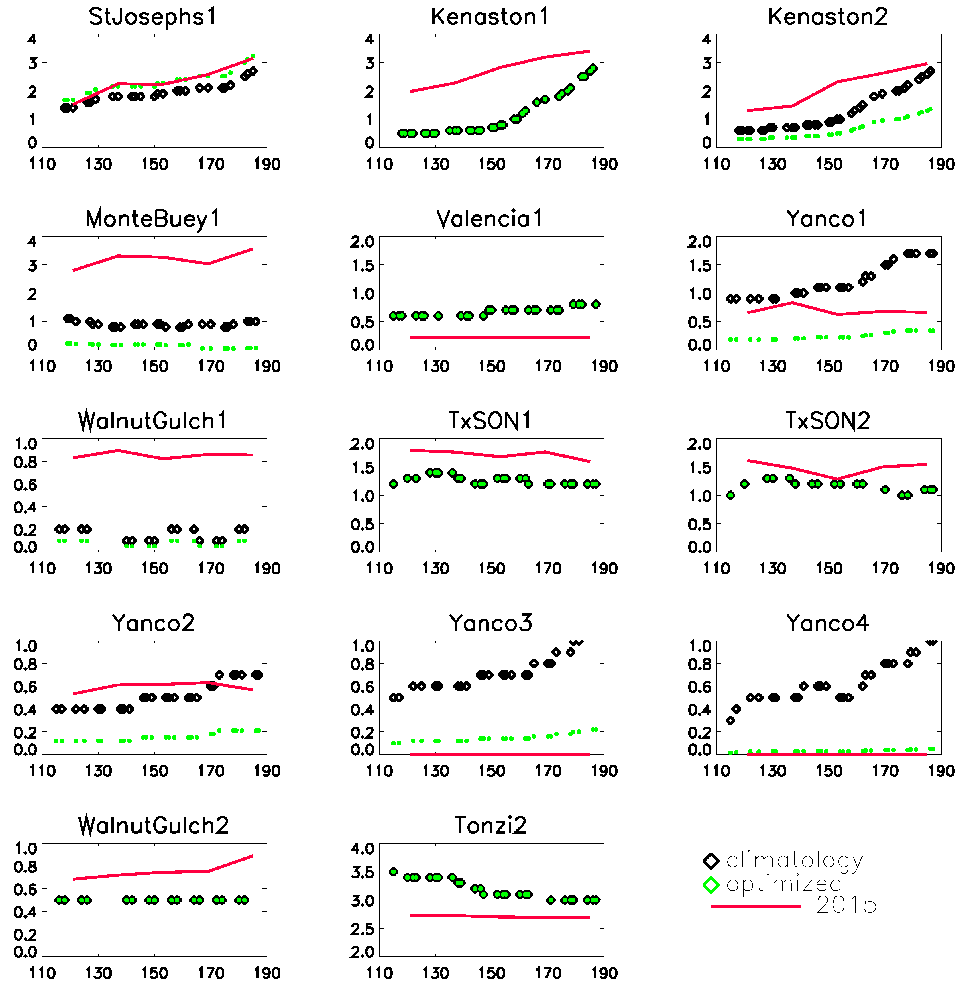
- In about half of the cases, the search of the minimum cost did not require the revision of the climatology VWC. A few cases exhibit seemingly a large revision, but in fact the revision is not significant. As the first example, the significant reductions in Yanco 3–4 are warranted. The climatology VWC reaches up to 1 kg/m2, which is too large for natural grassland. The 2015 MODIS data also predict small VWC (the VWC is set to zero in Figure 8 because the NDVI (normalized difference vegetation index) is −0.3: typically, NDVI smaller than 0.1 is associated with bare surface or rocks). The grassland VWC measured in the SGP99 campaign ranged from 0.1 to 0.5 kg/m2 only [41]. The second example is Walnut Gulch1. Although the size of f is large, this represents only a small revision from 0.2 to 0.1 kg/m2.
- -
- In Yanco 2, both the climatology and 2015 observation produce VWC of ~0.5 kg/m2, while the SMAP retrieval is smaller than 0.2 kg/m2. Possible errors in landcover classification may be the reason. Although the MODIS-based landcover database (mcd12q1) describes Yanco 2 as grassland, close examination indicates that the area is likely a cropland similar to Yanco 1. Because the forward models for grass vegetation were selected for this site and applied for retrieval, an error in retrieved VWC is anticipated. In the future, the forward model of crop vegetation will be tested on Yanco 2.
- -
- In the Monte Buey site, where a harvest ended around day 153, VWC is reduced with f changing from 0.3 to 0.05 (Figure 4). This is consistent with the expectation of post-harvest conditions. For this site, f was estimated for two separate time windows unlike the other sites where only one f was estimated.
- -
- The magnitude of the retrieved VWC in Monte Buey is only 20% of the climatology. A potential cause is that the forward model does not simulate the large undulations in σ0 associated with the effects by periodic crop rows (Figure 4). The minimization of the cost function could have lowered the retrieved VWC to best match the SMAP data. As a separate matter, why the 2015 VWC is so large and why it does not capture the effect of the harvest are unclear. An explanation may be that the conversion from NDVI to VWC is one formula regardless of the crop type, which may not be suitable for the dominant bean crop of the site.
- -
- In St. Josephs, the retrieved VWC is larger than the climatology, and the retrieval matches the 2015 VWC well. In Yanco1, the retrieval revises the climatology to the lower VWCs. The reduction is consistent with the comparison that the 2015 VWC is smaller than the climatology. However such consistency is not found in Kenaston 2.
- -
- The revision factor f is larger for croplands than non-croplands if the above rectification for the Yanco 2–4 and Walnut Gulch1 sites is taken into account. This agrees with the expectation because croplands experience large interannual changes and the climatology VWC ancillary may need revision.
5. Conclusions
Acknowledgments
Author Contributions
Conflicts of Interest
References
- Friesen, J.C.; Steele-Dunne, S.C.; van de Giesen, N. Diurnal differences in global ERS backscatter. IEEE Trans. Geosci. Remote Sens. 2012, 50, 2595–2602. [Google Scholar] [CrossRef]
- Oki, T.; Kanae, S. Global hydrological cycles and world water resources. Science 2006, 313, 1068–1072. [Google Scholar] [CrossRef] [PubMed]
- Schlesinger, W.H.; Jasechko, S. Transpiration in the global water cycle. Agric. For. Meteorol. 2014, 189, 115–117. [Google Scholar] [CrossRef]
- McNairn, H.; Boisvert, J.; Major, D.; Gwyn, G.; Brown, R.; Smith, A. Identification of agricultural tillage practices from C-band radar backscatter. Can. J. Remote Sens. 1996, 22, 154–163. [Google Scholar] [CrossRef]
- Azzari, G.; Lobell, D.B. Satellite-based classification of tillage practices in the US. In Proceedings of the AGU Fall meeting, New Orleans, LA, USA, 11–15 December 2017. [Google Scholar]
- Jackson, T.J.; Schmugge, T.J.; Wang, J.R. Passive microwave sensing of soil moisture under vegetation canopies. Water Resour. Res. 1982, 18, 1137–1142. [Google Scholar] [CrossRef]
- Attema, E.; Ulaby, F.T. Vegetation modeled as a water cloud. Radio Sci. 1978, 13, 357–364. [Google Scholar] [CrossRef]
- Pierdicca, N.; Pulvirenti, L.; Bignami, C. Soil moisture estimation over vegetated terrains using multitemporal remote sensing data. Remote Sens. Environ. 2010, 114, 440–448. [Google Scholar] [CrossRef]
- Theis, S.W.; Blanchard, B.J.; Blanchard, A.J. Utilization of active microwave roughness measurements to improve passive microwave soil-moisture estimates over bare soils. IEEE Trans. Geosci. Remote Sens. 1986, 24, 334–339. [Google Scholar] [CrossRef]
- Konings, A.G.; Piles, M.; Rotzer, K.; Chan, S.T.K.; McColl, K.A.; Entekhabi, D. Vegetation optical depth and scattering albedo retrieval using time series of dual-polarized L-band radiometer observations. Remote Sens. Environ. 2016, 172, 178–189. [Google Scholar] [CrossRef]
- Calvet, J.C.; Wigneron, J.P.; Walker, J.; Karbou, F.; Chanzy, A.; Albergel, C. Sensitivity of passive microwave observations to soil moisture and vegetation water content: L-band to W-band. IEEE Trans. on Geosci. Remote Sens. 2011, 49, 1190–1199. [Google Scholar] [CrossRef]
- Fernandez-Moran, R.; Al-Yaari, A.; Mialon, A.; Mahmoodi, A.; al Bitar, A.; de Lannoy, G.; Rodriguez-Fernandez, N.; Lopez-Baeza, E.; Kerr, Y.; Wigneron, J.-P. SMOS-IC: An alternative SMOS soil moisture and vegetation optical depth product. Remote Sens. 2017, 9, 21. [Google Scholar] [CrossRef]
- Wigneron, J.P.; Parde, M.; Waldteufel, P.; Chanzy, A.; Kerr, Y.; Schmidl, S.; Skou, N. Characterizing the dependence of vegetation model parameters on crop structure, incidence angle, and polarization at L-band. IEEE Trans. Geosci. Remote Sens. 2004, 42, 416–425. [Google Scholar] [CrossRef]
- Santi, E.; Paloscia, S.; Pampaloni, P.; Pettinato, S.; Nomaki, T.; Seki, M.; Sekiya, K.; Maeda, T. Vegetation water content retrieval by means of multifrequency microwave acquisitions from AMSR2. IEEE J. Sel. Top. Appl. Earth Observ. Remote Sens. 2017, 10, 3861–3873. [Google Scholar] [CrossRef]
- Parrens, M.; Wigneron, J.P.; Richaume, P.; Mialon, A.; al Bitar, A.; Fernandez-Moran, R.; Al-Yaari, A.; Kerr, Y.H. Global-scale surface roughness effects at L-band as estimated from SMOS observations. Remote Sens. Environ. 2016, 181, 122–136. [Google Scholar] [CrossRef]
- Hunt, E.R.; Li, L.; Yilmaz, M.T.; Jackson, T.J. Comparison of vegetation water contents derived from shortwave-infrared and passive-microwave sensors over central Iowa. Remote Sens. Environ. 2011, 115, 2376–2383. [Google Scholar] [CrossRef]
- Kim, Y.; Jackson, T.J.; Bindlish, R.; Lee, H.Y.; Hong, S.Y. Radar vegetation index for estimating the vegetation water content of rice and soybean. IEEE Geosci. Remote Sens. Lett. 2012, 9, 564–568. [Google Scholar]
- Arii, M.; van Zyl, J.J.; Kim, Y. A general characterization for polarimetric scattering from vegetation canopies. IEEE Trans. Geosci. Remote Sens. 2010, 48, 3349–3357. [Google Scholar] [CrossRef]
- Balenzano, A.; Mattia, F.; Satalino, G.; Davidson, M.W.J. Dense temporal series of C- and L-band SAR data for soil moisture retrieval over agricultural crops. IEEE J. Sel. Top. Appl. Earth Observ. Remote Sens. 2011, 4, 439–440. [Google Scholar] [CrossRef]
- Pathe, C.; Wagner, W.; Sabel, S.; Doubkova, M.; Basara, J.B. Using ENVISAT ASAR Global Mode data for surface soil moisture retrieval over Oklahoma, USA. IEEE Trans. Geosci. Remote Sens. 2009, 47, 468–480. [Google Scholar] [CrossRef]
- Dubois, P.C.; van Zyl, J.J.; Engman, E.T. Measuring soil moisture with imaging radars. IEEE Trans. Geosci. Remote Sens. 1995, 33, 915–926. [Google Scholar] [CrossRef]
- Kim, S.B.; Tsang, L.; Johnson, J.T.; Huang, S.; van Zyl, J.J.; Njoku, E.G. Soil moisture retrieval using time-series radar observations over bare surfaces. IEEE Trans. Geosci. Remote Sens. 2012, 50, 1853–1863. [Google Scholar] [CrossRef]
- Oh, Y.; Sarabandi, K.; Ulaby, F.T. An empirical model and an inversion technique for radar scattering from bare soil surfaces. IEEE Trans. Geosci. Remote Sens. 1992, 30, 370–382. [Google Scholar] [CrossRef]
- Kim, S.B.; van Zyl, J.J.; Johnson, J.T.; Moghaddam, M.; Tsang, L.; Colliander, A.; Dunbar, R.S.; Jackson, T.K.; Jaruwatanadilok, S.; West, R.; et al. Surface soil moisture retrieval using the L-band synthetic aperture radar onboard the Soil Moisture Active Passive (SMAP) satellite and evaluation at core validation sites. IEEE Trans. Geosci. Remote Sens. 2017, 55, 1897–1914. [Google Scholar] [CrossRef]
- Kim, S.B.; Moghaddam, M.; Tsang, L.; Burgin, M.; Xu, X.; Njoku, E.G. Models of L-band radar backscattering coefficients over the global terrain for soil moisture retrieval. IEEE Trans. Geosci. Remote Sens. 2014, 52, 1381–1396. [Google Scholar] [CrossRef]
- Tabatabaeenejad, A.; Burgin, M.; Moghaddam, M. Potential of L-band radar for retrieval of canopy and subcanopy parameters of boreal forests. IEEE Trans. Geosci. Remote Sens. 2012, 50, 2150–2160. [Google Scholar] [CrossRef]
- Huang, H.T.; Kim, S.B.; Tsang, S.; Xu, X.L.; Liao, T.H.; Jackson, T.J.; Yueh, S.H. Coherent model of L-band radar scattering by soybean plants: Model development, validation and retrieval. IEEE J. Sel. Top. Appl. Earth Observ. Remote Sens. 2016, 9, 272–284. [Google Scholar] [CrossRef]
- Kim, S.B.; Arii, M.; Jackson, T.J. Modeling L-band synthetic aperture radar observations through dielectric changes in soil moisture and vegetation over shrublands. J. Sel. Top. Appl. Earth Observ. Remote Sens. 2017. [Google Scholar] [CrossRef]
- Liao, T.H.; Kim, S.B.; Tan, S.; Tsang, S.; Su, C.X.; Jackson, T.J. Multiple scattering effects with cyclical terms in active remote sensing of vegetated surface using vector radiative transfer theory. IEEE J. Sel. Top. Appl. Earth Observ. Remote Sens. 2016, 9, 1414–1429. [Google Scholar] [CrossRef]
- Lang, R.H.; Sidhu, J.S. Electromagnetic backscattering from a layer of vegetation: A discrete approach. IEEE Trans. Antenn. Propag. 1983, 1, 62–71. [Google Scholar] [CrossRef]
- Huang, S.; Tsang, L.; Njoku, E.G.; Chen, K.S. Backscattering coefficients, coherent reflectivities, emissivities of randomly rough soil surfaces at L-band for SMAP applications based on numerical solutions of Maxwell equations in three-dimensional simulations. IEEE Trans. Geosci. Remote Sens. 2010, 48, 2557–2567. [Google Scholar] [CrossRef]
- Burgin, M.; Clewley, D.; Lucas, R.; Moghaddam, M. A generalized radar backscattering model based on wave theory for multilayer multispecies vegetation. IEEE Trans. Geosci. Remote Sens. 2011, 49, 4832–4845. [Google Scholar] [CrossRef]
- Konings, A.G.; McColl, K.A.; Piles, M.; Entekhabi, D. How many parameters can be maximally estimated from a set of measurements? IEEE Geosci. Remote Sens. Lett. 2015, 12, 1081–1085. [Google Scholar] [CrossRef]
- Oh, Y.; Sarabandi, K.; Ulaby, F.T. Semi-empirical model of the ensemble-averaged differential Mueller matrix for microwave backscattering from bare soil surfaces. IEEE Trans. Geosci. Remote Sens. 2002, 40, 1348–1355. [Google Scholar] [CrossRef]
- Jackson, T.J.; Hsu, A.Y. Soil moisture and TRMM microwave imager relationships in the Southern Great Plains 1999 (SGP99) experiment. IEEE Trans. Geosci. Remote Sens. 2001, 39, 1632–1642. [Google Scholar] [CrossRef]
- McNairn, H.; Jackson, T.J.; Wiseman, G.; Belair, S.; Bullock, P.; Colliander, A.; Cosh, M.H.; Kim, S.-B.; Magagi, R.; Moghaddam, M.; et al. The Soil Moisture Active Passive Validation Experiment 2012 (SMAPVEX12): Pre-launch calibration and validation of the SMAP Satellite. IEEE Trans. Geosci. Remote Sens. 2015, 53, 2784–2801. [Google Scholar] [CrossRef]
- Colliander, A.; Jackson, T.J.; Bindlish, R.; Chan, S.; Das, N.; Kim, S.B.; Cosh, M.B.; Dunbar, R.S.; Dang, L.; Pashaian, L.; et al. Validation of SMAP surface soil moisture products with core validation sites. Remote Sens. Environ. 2016, 191, 215–231. [Google Scholar] [CrossRef]
- Whitt, M.W.; Ulaby, F.T. Radar response of periodic vegetation canopies. Int. J. Remote Sens. 1994, 15, 1813–1848. [Google Scholar] [CrossRef]
- Toure, A.; Thomson, K.P.B.; Edwards, G.; Brown, R.J.; Brisco, B.G. Adaptation of the MIMICS backscattering model to the agricultural context—Wheat and canola at L and C bands. IEEE Trans. Geosci. Remote Sens. 1994, 32, 47–61. [Google Scholar] [CrossRef]
- Chiu, T.; Sarabandi, K. Electromagnetic scattering from short branching vegetation. IEEE Trans. Geosci. Remote Sens. 2000, 38, 911–925. [Google Scholar] [CrossRef]
- Jackson, T.J.; le Vine, D.M.; Hsu, A.Y.; Oldak, A.; Starks, P.J.; Swift, C.T.; Isham, J.D.; Haken, M. Soil moisture mapping at regional scales using microwave radiometry: The Southern Great Plains hydrology experiment. IEEE Trans. Geosci. Remote Sens. 1999, 37, 2136–2151. [Google Scholar] [CrossRef]


| Michigan Tower | SGP99 | SMAPVEX12 | SJV | SMAP | |
|---|---|---|---|---|---|
| Spatial Resolution | NA | ~800 m | 10 m | 10 m | 3 km |
| # Time Series | 10 | 6 | 13 | 14 | ~25 |
| In situ roughness Availability | yes | yes | yes | yes | no |
| In situ VWC Availability | Not applicable | yes | yes | yes | no |
| Landcover | Bare soil | Pasture | Pasture,wheat, soybean,corn, canola | Shrub | Pasture, Wheat, soybean |
| Landcover | RMS of Measured Signal | Bias | RMSE | Correlation | |
|---|---|---|---|---|---|
| Coefficient | p-Value | ||||
| Bare | 2.04 | 0.12 | 0.49 | 0.99 | 0.006 |
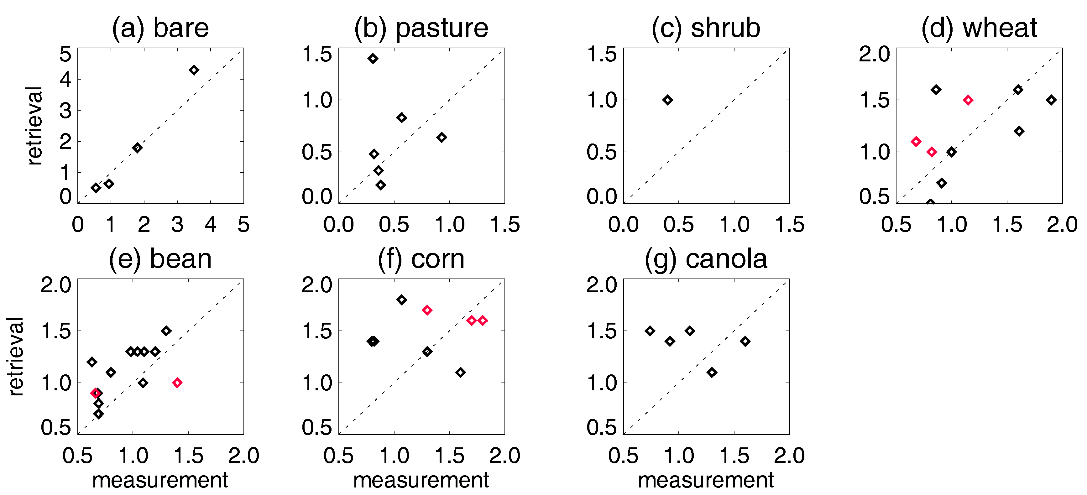
| Pasture (if excluding outlier *) | 0.53 | 0.16 (−0.02) | 0.53 (0.23) | −0.004 (0.58) | 0.994 (0.303) |
| Wheat | 1.20 | 0.036 | 0.39 | 0.54 | 0.105 |
| Bean | 0.98 | 0.16 | 0.28 | 0.59 | 0.035 |
| Corn | 1.37 | 0.034 | 0.63 | −0.16 | 0.677 |
| Canola | 1.17 | 0.25 | 0.50 | −0.42 | 0.479 |
| Cropland | St. Josephs | Kenaston1 | Kenaston2 | Monte Buey | Valencia | Yanco1 | ||
|---|---|---|---|---|---|---|---|---|
| Retrieval | 3.1 | 1.3 | 1.2 | 2.1 | 3.9 | 3.7 | ||
| Noncrop land | Walnut Gulch1 grass | TxSON1 savanna | TxSON2 savanna | Yanco2 grass | Yanco3 grass | Yanco4 grass | Walnut Gulch2 shrub | Tonzi woody savanna |
| Retrieval | 1.7 | 2.0 | 1.4 | 2.0 | 1.9 | 0.34 | 0.26 | 2.5 |
| Wheat HH | Canola HH | Soybean HH | ||||
|---|---|---|---|---|---|---|
| Surface (dB) | −20.8 | −20.0 | −25.3 | −18.1 | −26.1 | −27.4 |
| Double bounce (dB) | −19.4 | −18.4 | −16.8 | −13.1 | −28.0 | −19.0 |
| Volume (dB) | −41.3 | −41.3 | −17.1 | −14.1 | ||
| at VWC (kg/m2) | 1.5 | 2.3 | 1.9 | 8.0 | 0.10 | 0.54 |
| at Mv (m3/m3) | 0.2 | 0.25 | 0.25 | |||
| Cropland | St. Josephs | Kenaston 1 | Kenaston 2 | Monte Buey | Valencia | Yanco1 | ||
|---|---|---|---|---|---|---|---|---|
| Retrieval | +20% | 0 | −50% | −80% | 0 | −80% | ||
| Non cropland | Walnut Gulch1 grass | TxSON1 savanna | TxSON2 savanna | Yanco2 grass | Yanco3 grass | Yanco4 grass | Walnut Gulch2 shrub | Tonzi woody savanna |
| Retrieval | −50% | 0 | 0 | −70% | −90% | −95% | 0 | 0 |
© 2018 by the authors. Licensee MDPI, Basel, Switzerland. This article is an open access article distributed under the terms and conditions of the Creative Commons Attribution (CC BY) license (http://creativecommons.org/licenses/by/4.0/).
Share and Cite
Kim, S.-B.; Huang, H.; Liao, T.-H.; Colliander, A. Estimating Vegetation Water Content and Soil Surface Roughness Using Physical Models of L-Band Radar Scattering for Soil Moisture Retrieval. Remote Sens. 2018, 10, 556. https://doi.org/10.3390/rs10040556
Kim S-B, Huang H, Liao T-H, Colliander A. Estimating Vegetation Water Content and Soil Surface Roughness Using Physical Models of L-Band Radar Scattering for Soil Moisture Retrieval. Remote Sensing. 2018; 10(4):556. https://doi.org/10.3390/rs10040556
Chicago/Turabian StyleKim, Seung-Bum, Huanting Huang, Tien-Hao Liao, and Andreas Colliander. 2018. "Estimating Vegetation Water Content and Soil Surface Roughness Using Physical Models of L-Band Radar Scattering for Soil Moisture Retrieval" Remote Sensing 10, no. 4: 556. https://doi.org/10.3390/rs10040556