Snow Density and Ground Permittivity Retrieved from L-Band Radiometry: Melting Effects


1
Swiss Federal Research Institute WSL, CH-8903 Birmensdorf, Switzerland
2
Gamma Remote Sensing AG, CH-3073 Gümligen, Switzerland
*
Author to whom correspondence should be addressed.
Remote Sens. 2018, 10(2), 354; https://doi.org/10.3390/rs10020354
Submission received: 13 December 2017
/
Revised: 15 February 2018
/
Accepted: 21 February 2018
/
Published: 24 February 2018
(This article belongs to the Special Issue Snow Remote Sensing)
Abstract
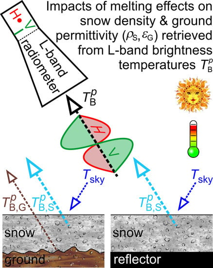
:Ground permittivity and snow density retrievals for the “snow-free period”, “cold winter period”, and “early spring period” are performed using the experimental L-band radiometry data from the winter 2016/2017 campaign at the Davos-Laret Remote Sensing Field Laboratory. The performance of the single-angle and multi-angle two-parameter retrieval algorithms employed during each of the aforementioned three periods is assessed using in-situ measured ground permittivity and snow density. Additionally, a synthetic sensitivity analysis is conducted that studies melting effects on the retrievals in the form of two types of “geophysical noise” (snow liquid water and footprint-dependent ground permittivity). Experimental and synthetic analyses show that both types of investigated “geophysical noise” noticeably disturb the retrievals and result in an increased correlation between them. The strength of this correlation is successfully used as a quality-indicator flag for the purpose of filtering out highly correlated ground permittivity and snow density retrievals. It is demonstrated that this filtering significantly improves the accuracy of both ground permittivity and snow density retrievals compared to corresponding reference in-situ data. Experimental and synthetic retrievals are performed in retrieval modes RM = “H”, “V”, and “HV”, where brightness temperatures from polarizations p = H, p = V, or both p = H and V are used, respectively, in the retrieval procedure. Our analysis shows that retrievals for RM = “V” are predominantly least prone to the investigated “geophysical noise”. The presented experimental results indicate that retrievals match in-situ observations best for the “snow-free period” and the “cold winter period” when “geophysical noise” is at minimum.
1. Introduction
Microwave remote sensing can provide necessary information on Cryosphere state parameters by quantifying radiation, heat, and mass fluxes through the terrestrial surface layer [1,2], which are determinative for exchange rates of water between land and atmosphere. As a consequence, emerging microwave remote sensing techniques have focused on obtaining global-scale information on parameters, such as snow cover [3,4,5], vegetation optical depth [6,7], ground freeze/thaw states [8,9,10], and soil moisture [11,12,13]. The availability of these recently observable state parameters improves forecasts of climate scenarios and the optimization of corresponding mitigation strategies. For instance, ground freeze/thaw and snow cover play a key role in hydrological, climatological, and ecological processes in northern latitudes. Variations in their seasonal cycle have a major impact on the annual carbon balance [14,15] and vegetation growth [16]. Snow qualities, such as density, influence the energy budget through albedo feedbacks [17], and control thermal insulation of the soil [18], which in turn affects river run-off in the northern hemisphere [19,20,21] and mountainous [22] regions. Beyond these, weather forecasting, environmental hazard warning, and food production benefit directly from microwave remote sensing data acquired through novel satellite missions. Examples of recent space missions at L-band dedicated to the observation of the Earth’s water cycle include the European Space Agency’s (ESA) launch of the second Earth explorer Soil Moisture and Ocean Salinity (SMOS) mission [12,23,24] in 2009, and the Soil Moisture Active Passive (SMAP) mission [25] implemented by the National Aeronautics and Space Administration (NASA) in 2015. Spaceborne remote sensing also at visible and higher microwave frequencies has been used, for example, for large-scale monitoring of snow cover over the Northern hemisphere [26], Alpine regions [27], and the Arctic [28].
Despite these developments, full exploitation of available microwave data in terms of information on snow-covered ground is yet to be implemented in corresponding retrieval schemes. Further research is needed to update and develop microwave retrieval schemes, explore their sensitivities with respect to “geophysical noise” sources—understood as radiative transfer effects neglected in underlying emission models—and develop methods that are capable of assessing retrieval performances. The central theme of the research presented here is the tackling of the latter two issues. This is seen as a continuation of a series of recent research [29,30,31] on the application of passive L-band data to gain remote information on snow mass-density and the permittivity of the underlying ground used, for instance, to characterize freeze/thaw states. It is noteworthy that there have been several attempts to specifically retrieve snow density [32,33,34] and ground permittivity [32,35,36] using microwave remote sensing; however, to the best of the authors’ knowledge, all of them are based on active remote sensing and employ the (often semi-empirical) relationship between measured backscatter and properties of snowpack and/or underlying ground.
The research for using passive L-band data for the retrieval of snow column properties and ground dielectric permittivity began in 2014 with the development of an emission model consisting of parts of the Microwave Emission Model of Layered Snowpack “MEMLS” [37], coupled with components of the L-band Microwave Emission of the Biosphere “L-MEB” model [38]. The resulting emission model is specifically designed for the simulation of L-band brightness temperatures emitted by snow-covered ground. Model evaluations lay the foundation for the recognition that, despite the predominant transparency of dry snow at L-band frequencies, brightness temperatures are still sensitive to the mass-density of snowpack via refraction and impedance matching. Furthermore, the formulation of the aforementioned L-band-specific emission model is simple enough for its use in an iterative retrieval approach. These two considerations have led to the development of the two-parameter retrieval scheme [30] to estimate bottom-layer snow density and ground permittivity from L-band brightness temperatures. The first assessment of retrievals achieved by means of tower-based passive L-band measurements performed at the Finnish Meteorological Institute Arctic Research Center (FMI-ARC), Sodankylä, Finland is presented in [31]. For dry-snow conditions over frozen ground, this experimental study revealed successful retrievals in most cases, whereas retrieval performance noticeably drops for warmer periods accompanied by partial snow and ground melting. The drop in performance is explained by the increased complexity of the observed scenes that were not captured by the emission model used in the retrieval scheme. Impacts on retrievals caused by resultant so-called “geophysical noise” is analyzed in [39]. This synthetic analysis explores the sensitivity of retrievals with respect to selected types of “geophysical noise”, namely, (i) the parameterization of ground roughness, and (ii) scenarios of differing density distributions across snow heights.
It should be noted that the sensitivity of retrievals with respect to specific types of “geophysical noise”, held to be most relevant during warmer winter periods, has not been explored to date. This includes, in particular, liquid snow water and the spatial heterogeneity of ground permittivity, both of which were identified as the prominent sources of “geophysical noise” that reduced retrieval quality for melting phases that were observed during the prior mentioned FMI-ARC campaign [31]. Accordingly, the overall rationale of the present research is to study the disturbative effects of melting on retrievals derived from L-band brightness temperatures. It is noteworthy that in this paper, snow liquid water is seen as a disturbative factor on retrievals, while the companion paper [40] investigates the possibility of estimating snow liquid water using the sensitivity of L-band brightness temperatures to the snow moisture investigated in [41]. Therefore, the reader is strongly advised to consult the companion paper [40], which is closely linked to the analyses presented here.
The subsequently presented research includes model-based and experimental investigations of the sensitivities of retrievals with respect to snow liquid water and variability of ground permittivity observed by a radiometer operated in “swath scanning” mode, based on the view that footprint areas at different nadir angles are not congruent (see Figure 1 in [42]). A comprehensive description of the measurement campaign conducted at the Davos-Laret Remote Sensing Field Laboratory (Switzerland), the processing of the calibrated L-band brightness temperatures, and the in-situ reference data are outlined in detail in [41]. Section 2 provides selected information on the measurement configuration, and the in-situ and radiometry data collection that is necessary for this study. The methods used to achieve two-parameter retrievals and employed in the two types of synthetic sensitivity studies are outlined in Section 3. The results of the simulated retrieval sensitivities with respect to snow liquid water and ground permittivities varying among footprints observed at different nadir angles (-dependent ground permittivities) are presented in Section 4. Section 5 contains measurement-based retrievals as compared with in-situ references, including links between model-based and experimental findings, followed by the presentation of a novel approach to the rating of the reliabilities of retrievals, even without making comparisons to in-situ references.
2. Data Sets
2.1. Test Site
The Davos-Laret Remote Sensing Field Laboratory (48°50′53′′N 9°52′19′′E) in Switzerland is a area with an approximate elevation of 1450 m above sea level. The ground is mostly flat with some smooth slopes on the north-western side of the site. The valley, including the site area, is surrounded by mountains with an average height difference of ~400 m with respect to the site. The site area is surrounded by Lake Schwarz on the north-western side, canopy forest on the south-eastern side, and local buildings on the north-eastern and south-western sides. The spring- and summertime vegetation cover of the site is grass. The 2016/2017 measurement campaign, whose data is used in this paper, started in late autumn 2016 on 27 November and ended in early spring on 15 March. The snow cover was continuously present from 3 January 2017 until the end of March 2017 with the lowest and highest in-situ snow density measurements ranging from to . Further details on the seasonal snow cover and structure of the Davos-Laret site can be found in [43] and references therein.
2.2. In-Situ Measurements
In-situ measurements performed during the first operation of the Davos-Laret field laboratory in Winter 2016/2017 are presented here, focusing on those that are used to evaluate and analyze the snow density and ground permittivity retrievals from L-band radiometry. A more comprehensive description of these in-situ measurements can be found in [41].
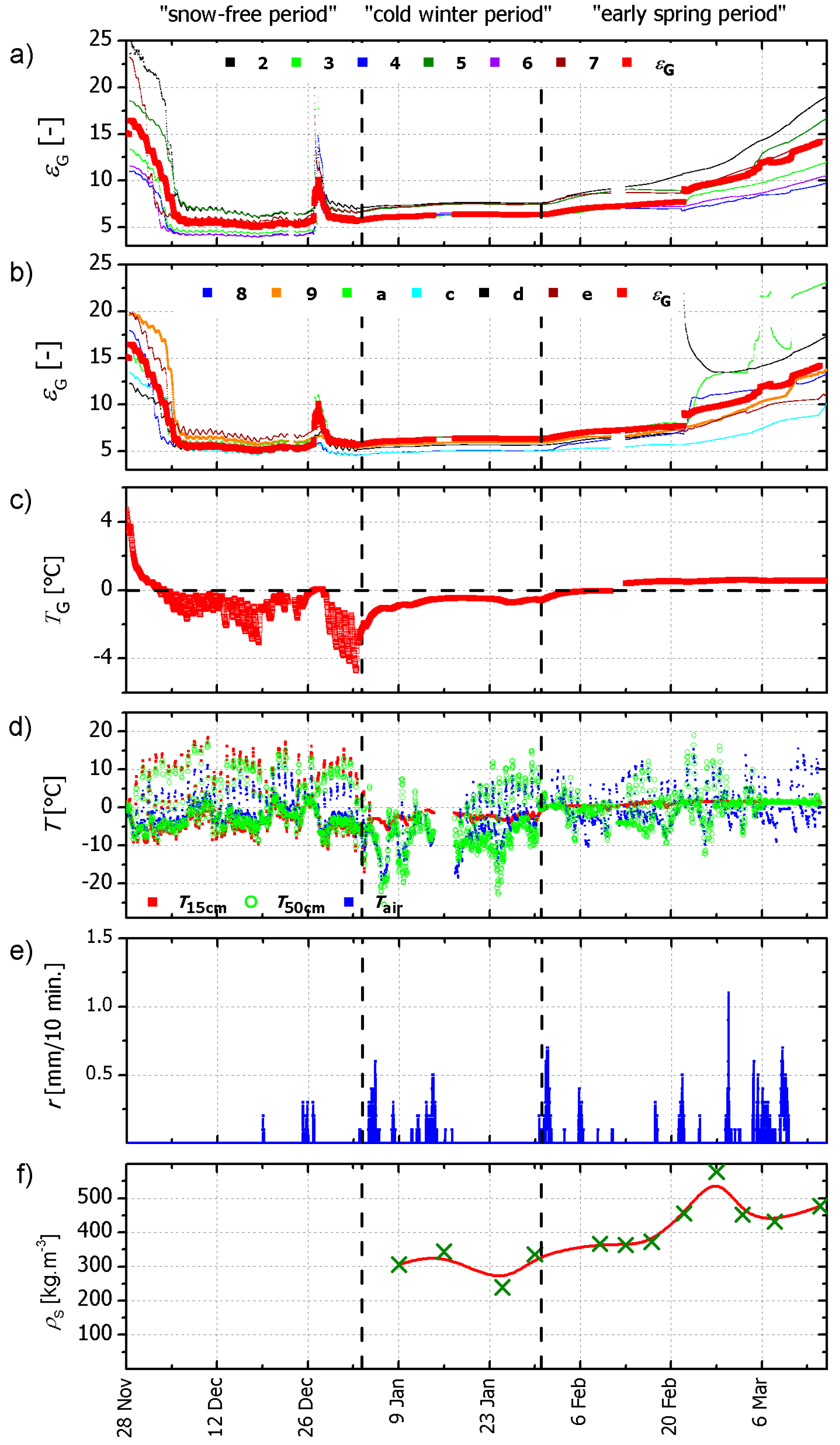
Ground permittivities and temperatures were measured automatically every five minutes using SMT-100 sensors [44] installed approximately 5 cm below the ground’s surface. The SMT-100 sensors, indicated by red squares in Figure 1, use a ring oscillator, in which a steep pulse, emitted by a line driver, travels along a closed transmission line buried in soil. The permittivity of the medium is computed based on the travel time of the pulse. The temperature of the medium is also measured by the SMT-100 using a digital temperature sensor. Figure 2a–f show the in-situ measurements of ground permittivity, ground and air temperatures, precipitation, and bottom-layer snow density. More details on these measurements can be found in the caption of Figure 2. It is worth reminding that the snow profile measurements were conducted approximately once a week, after the first major snow fall on 3 January, using a snow cutter with a depth resolution of 10 cm. The first and last snow profile measurements were conducted on 8 January and 22 March, respectively.
The first week of the in-situ time series reveals the rapid freezing of the bare ground surface. Naturally, this results from the low diurnal heat input to the ground that is associated with air temperatures mostly below the freezing point. Figure 2c,d indicate that while the temperatures above ground still show short-term peaks above during afternoons, ground temperatures steadily decrease until they fall below the freezing point. However, at the latest by the middle of December, ground permittivities measured by all of the sensors drop to the range 4 to 7, indicating that at least the top 5 cm of the ground is completely frozen. Around 26 December, a slight thawing event takes place as the result of increased time-integrated heat input and precipitation to the still snow-free bare ground. This is reflected in approaching the threshold and the increased recorded that indicates increased liquid water in the ground’s surface.
Figure 2a,b show that during the “snow-free period” the ground is fully frozen with slight daily fluctuations in resulting from partial surface melting caused by increased heat input during cloudless afternoons and refreezing overnight. These fluctuations disappear with the onset of snow cover on 3 January due to thermal insulation of the accumulating dry snow.
According to Figure 2a,b, the thawing of the ground starts gradually with the beginning of the “early spring period” after 31 January. By the middle of March, the ground has almost entirely thawed. It is noticeable that the deviations between permittivity readings of the different sensors increase with the on-going thawing process, indicating that heterogeneity of ground permittivity is significantly higher under such transient ground conditions.
2.3. Radiometry Data
An ELBARA-II radiometer [45] was used to measure L-band brightness temperatures in the protected frequency band 1400 MHz–1427 MHz at both vertical and horizontal polarizations p = H, V. The instrument was mounted on an eight-meter tower and was equipped with tracking systems that permitted automated observations of at discrete nadir angles and azimuth directions. The tracking system was configured to perform sequential measurements at the eight nadir angles (Figure 1). This measurement cycle was performed once an hour throughout the campaign. Sky measurements, which as explained in Section 4.1 in [41], are necessary for the computation of calibrated brightness temperatures, were initiated manually during precipitation-free times, every other day when possible and done at nadir angle .
A detailed explanation of the conversion of ELBARA-II raw data to calibrated brightness temperatures can be found in [41]. During the 2016/2017 winter campaign, L-band radiometry was performed over areas with a metal reflector placed on the ground. These measurements and the resulting snow liquid water content retrievals are thoroughly described in the companion paper [40].
3. Methodology
The L-band-Specific Microwave Emission Model of Layered Snowpacks, henceforth denoted as “LS—MEMLS”, is the fundamental modeling tool that is employed here to retrieve dry snow mass-density and ground permittivity based on simulated and measured brightness temperatures . “LS—MEMLS” is used in its single-layer configuration that assumes snow to be dry whenever it is used as the forward emission model to retrieve and . Conversely, more general versions of “LS—MEMLS” are applied to simulate and generate synthetic measurements considering multiple snow layers that include liquid water. While the present text provides extensive explanations regarding “LS—MEMLS”, its general form, as well as its single dry-snow layer version, are comprehensively explained in Section 5.1 in [41]. The reader is also referred to [30], in which both the specific single-layer dry-snow version of “LS—MEMLS” and the thereupon based retrieval of are outlined.
Section 3.1 explains the methodology used to achieve multi-angle retrievals at retrieval modes RM from elevation scan sets of L-band brightness temperatures measured over a range of nadir angles as is provided by airborne and spaceborne radiometers, such as the SMOS satellite. A similar two-parameter retrieval approach is explained and employed in [30,31,39] for both synthetic and experimental retrieval analyses. The refinement of the multi-angle retrieval used in this work is based on the consideration of different weights that are applied to measurements , according to their uncertainty. Section 3.2 outlines the methodology used to achieve footprint-specific retrievals based on the corresponding measurements performed at a specific individual nadir angle as is the case for SMAP data. The resulting single-angle retrievals in the present study are mainly used to explore variation in ground permittivities among footprints observed at . Section 3.3 explains the methodologies used to investigate the sensitivities of multi-angle retrievals with respect to snow moisture and with respect to -dependent ground permittivities. The sensitivities of L-band brightness temperatures with respect to snow liquid water column are thoroughly discussed in Section 5.2 in [41]. Note that estimates of retrieval sensitivity to -dependent ground permittivities is important when using elevation scan sets acquired with a radiometer operated in “swath scanning” mode [42].
3.1. Multi-Angle Retrieval Approach
In physically-based retrieval approaches (such as the SMOS level 2 soil moisture retrieval), parameters of interest are conventionally estimated as the solution of an overdetermined system of equations. In other words, these parameters are estimated by optimally fitting modeled signatures to corresponding remote sensing observations. Thereto, aberrations between modeled and remotely sensed data are expressed by a cost function CF, which includes the desired retrieval parameters. In the specific case of the retrieval approach used here to estimate snow density and ground permittivity from multi-angle L-band brightness temperatures at horizontal (p = H) and vertical (p = V) polarizations, the cost function is defined as:
The equation above represents the sum of squared differences between observed elevation scan sets and corresponding simulations for given values of and. Further inputs (see Figure 9 in [41]) that are used in the single dry-snow layer version of “LS—MEMLS” for the simulation of are air humidity , rain rate , elevation of the Davos-Laret site , and the HQN ground roughness parameters = . Air temperatures are measured by ELBARA-II, and ground temperatures are represented by the means of the in-situ measurements along the two transects shown in Figure 1. Assumptions made on snow temperature and snow depth are irrelevant for dry snow (with volumetric liquid water-content ) because of negligible snow emission in this case.
Through a global numerical minimization process based on tuning the values of the retrieval parameters and , the cost function in Equation (1) is minimized and the corresponding minimized pair of values is taken as the result of the retrieval. Two-parameter retrievals are performed for three different “retrieval modes” (first introduced and employed in [39]) with RM = “H”, “V” including either for p = H or V, and RM = “HV” using both polarizations. When considering that are acquired with ELBARA-II operating in a “swath scanning" mode (Figure 1 in this paper and in [42]), multi-angle retrievals are “effective” values of snow mass-density and ground permittivity representative of the entire area covered by the footprints observed at .
The denominator in the cost function assigns different weights to according to their uncertainty, which is understood as the sum of the radiometer assembly’s (RMA) inherent uncertainty and the error imposed by non-thermal noise entering the antenna. The greater the value of the denominator in Equation (1), the lower the weight that is assigned to a specific measurement . In the case of ELBARA-II, the radiometer uncertainty is [45,46]. Non-thermal RFI, , is estimated from the non-Gaussianity of the probability density function (PDF) of the raw-data voltage sample associated with a measurement . Highly RFI-corrupted (with coefficients of determination between the PDF of the measured raw-data voltage sample and the perfect Gaussian PDF) are excluded from retrievals and thus ignored in the cost function , as defined in Equation (1). This approach, used to mitigate and filter RFI, is explained in detail in Section 4.2 in [41]. The consideration of , as the non-thermal RFI, in Equation (1) is seen as an important improvement to the two-parameter retrieval procedure that is used in previous papers [30,31,39].
3.2. Single-Angle Retrieval Approach
Similar to the physically-based multi-angle retrieval, a physically-based single-angle retrieval approach relies on optimally fitting modeled signatures to corresponding observational data. When the objective is to estimate the two specific parameters from the two measurements and performed at the respective single nadir angle , the mathematical system to solve is no longer overdetermined—unlike the case for the corresponding multi-angle retrievals explained in Section 3.1. Instead, retrieving footprint-specific retrieval pairs consists of solving the following equation system for :
Obviously, only the retrieval mode RM = “HV” is applicable to achieve footprint-specific two-parameter retrievals because the mathematical system becomes underdetermined if only one of the two polarizations is used (two unknowns and one equation). Again, the single-layer dry-snow configuration of “LS—MEMLS” with the same auxiliary inputs as used in the multi-angle retrieval (Section 3.1) is employed to simulate and of the footprint at .
are expected to be affected significantly by (i) the uncertainties of the two measurements and , and (ii) imperfect modeling of footprint brightness temperatures and . In this respect, the multi-angular retrieval approach (Section 3.1) outperforms the single-angle retrieval approach. On the other hand, multi-angle retrievals employing “swath scanning“ measurements are expected to suffer at least as much from varying emission properties among the displaced footprint areas that are observed at different as, for instance, from special heterogeneous ground permittivity.
Single-angle retrieval pairs , which are physically meaningless, suggest either distorted footprint measurements , or the inadequate representation of the actual footprint emission achieved by the simulations . The latter can result when the single-layer dry-snow configuration of “LS—MEMLS” poses a severe over-simplification of the actual emission properties of the footprint observed at . This is mainly caused by (i) snow structural features of the order of the observation wavelength (), which cause volume scattering and/or absorption/emission, (ii) layers of ice and/or moist-snow especially when present at the ground-snow interface.
3.3. Sensitivity of Multi-Angle Retrievals to Snow Wetness and Ground Permittivity Varying among Footprints
Multi-angle two-parameter retrievals are derived from elevation scan sets of measured . The multi-angle retrieval approach (Section 3.1) employs the single-layer dry-snow configuration of “LS—MEMLS” (Section 5.1 in [41]) to simulate used in the cost function , as defined in Equation (1). Assuming snow to be homogeneous and dry can pose an oversimplification of reality, especially for mature snowpacks. As a consequence, the shortcomings of the forward emission model can cause retrieval distortion, which demands the model-based analysis of retrieval sensitivities. Such a study is presented in [39], where the sensitivities of retrievals are analyzed with respect to: (i) assumptions made on the ground-surface roughness parameterization, and (ii) digressions from a perfectly uniform mass-density profile across the snowpack. However, in both of these two analysis categories, the snowpack is assumed to be totally dry and the same ground permittivities are considered for all footprint areas associated with the different nadir angles of an elevation scan set . With this in mind, the analysis presented here, which highlights retrieval sensitivity with respect to “melting effects” such as snow liquid water column (Section 4.1), and varying ground permittivities among the elevation scans’ footprints at (Section 4.2), complements our previous work [39]. The methodologies that are employed are in close analogy to those used in [39], and are described through the rest of this section following the flowchart in Figure 3.
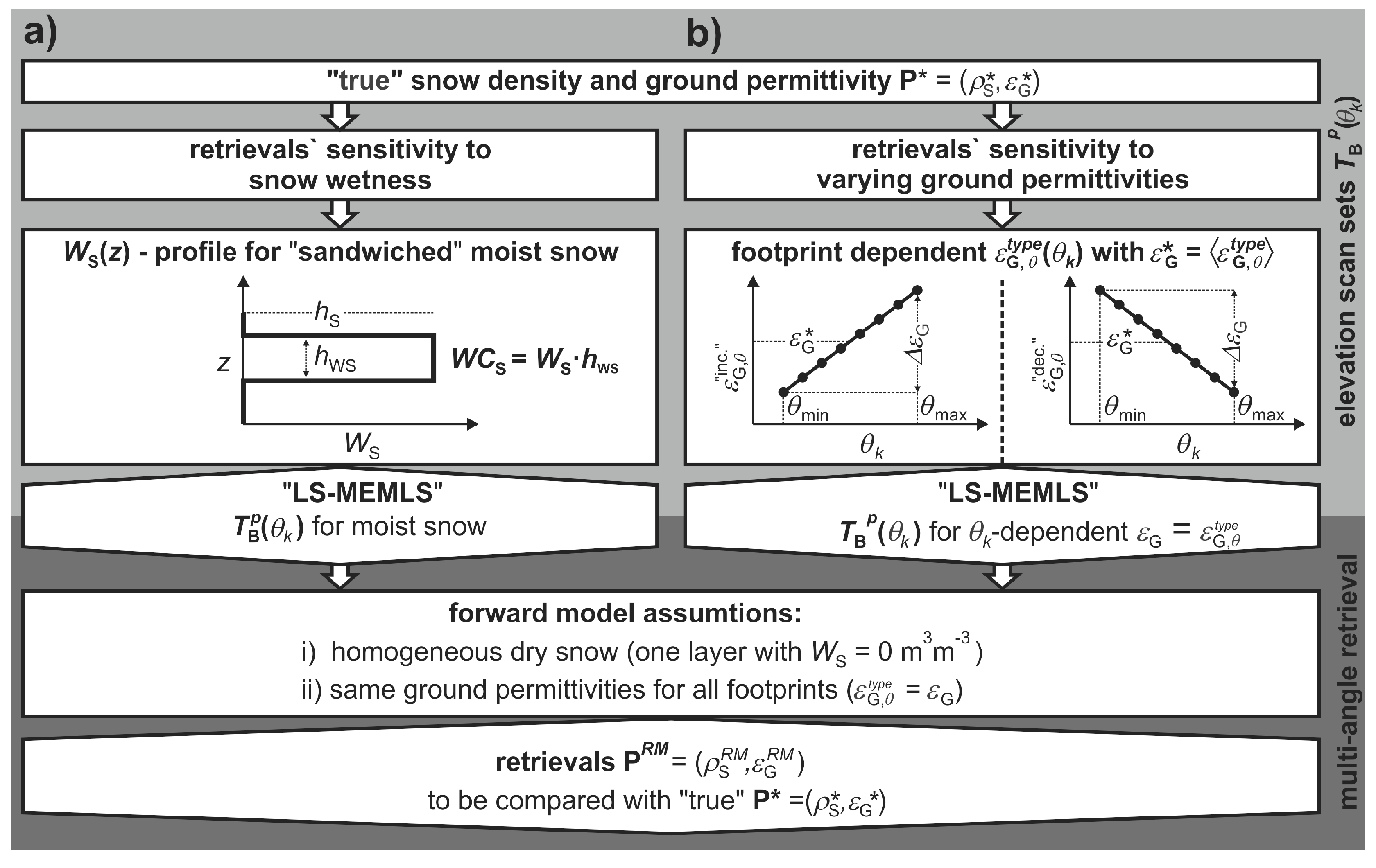
The model methodology used to investigate the impacts of snow liquid water column (Figure 3a) and -dependent ground permittivity (Figure 3b) consists of the two main steps overlaid in light and dark gray in the flowchart:
- The initial snow density and ground permittivity values , henceforth called “true” parameter values, together with a range of (i) snow liquid water column or (ii) footprint-specific ground permittivity values, are fed in “LS—MEMLS” to simulate scan sets (p = H, V; ) of brightness temperatures. These synthetic elevation scan sets , mimic L-band measurements of a (i) moist snowpack or (ii) dry snowpack over a ground with varying permittivities among footprints.
- Using the elevation scan sets in the multi-angle retrieval scheme (Section 3.1) to derive retrievals to be compared with the “true” parameter values .
Step 1 is different when it comes to retrieval sensitivities with respect to snow liquid water column , or with respect to footprint-dependent ground permittivity. However, once are available for the respective type of analysis, the same multi-angle retrieval (step 2) is applied to achieve for retrieval modes RM = “H”, “V”, and “HV”. It is once more emphasized that the retrieval approach assumes a dry () single-layer snowpack, and equal ground permittivities () for all of the footprints observed at nadir angle . Accordingly, any difference between retrievals and “true” values used to simulate scan sets is inherently interpreted as a measure of retrieval sensitivity to snow liquid water or varying ground permittivities among footprints at .
Parameter values that are commonly used to simulate (step 1) for both types of retrieval sensitivity analysis, and also in the subsequent retrieval (step 2), are the HQN ground roughness parameters = , temperatures of ground, snow, and air , and the eight discrete nadir angles . The different configurations of “LS—MEMLS” for the simulation of the synthetic elevation scan sets (step 1) associated with the two types of retrieval sensitivity analysis are subsequently outlined following the light gray shaded parts of the flowchart:
3.3.1. Elevation Scan Sets Representative of Moist Snow
Synthetic elevation scan sets , extractable to analyze the sensitivities of multi-angle retrievals with respect to snow liquid water column , are simulated following the steps in the light-gray shaded area of the flowchart in Figure 3a. The starting point is the specification of the pair of “true” values of dry snow mass-density and ground permittivity, respectively. Proceeding from this, the other inputs required in “LS—MEMLS” to simulate , representative of a snowpack with given liquid water column , are defined subsequently.
In Section 5.2 of [41], the scenarios “uniform”, “top”, “sandwiched”, and “bottom” of liquid water content profiles are considered to analyze the sensitivities of L-band brightness temperatures to snow liquid water column defined as snows volumetric liquid water content integrated over the entire snow depth . There, it is argued that the “sandwiched” scenario is the most realistic during “cold winter periods”—when successful retrievals are expected—because strong short-wave solar radiation penetrates the first few centimeters of dry snow and can cause partial subsurface melting. This phenomenon can be best called the “snow greenhouse effect” [41]. Accordingly, the sensitivity analyses presented here assume this scenario, modeled as three homogeneous snow layers with a wet layer of thickness within the snowpack. As is also shown in Section 5.2 in [41], simulated brightness temperatures are independent of the thicknesses of the two dry snow layers atop and below the “sandwiched” moist snow layer, as a direct consequence of almost negligible absorption in dry snow at L-band. This immediately implies that simulated elevation scan sets and, consequently, the thereon based estimates of retrieval sensitivities to , are independent of the assumption of the total snow height .
3.3.2. Elevation Scan Sets Representative of Ground Permittivities Varying among Footprints
Synthetic elevation scan sets , extractable to analyze the sensitivities of retrievals with respect to ground permittivities varying between footprints at different nadir angles , are simulated following the light-gray shaded area of the flowchart in Figure 3b. Again, the starting point is the specification of the pair of “true” values, followed by the preparation of other “LS—MEMLS” inputs that are needed to simulate . The impact of varying ground permittivity among footprints at is investigated here by means of two types: i) type = “inc.” is modeled as footprint permittivity linearly increasing with increasing nadir angles ; ii) type = “dec.” is modeled as footprint permittivity linearly decreasing with increasing . Formally, are expressed by the linear model:
For type = “inc.” (upper signs) and “dec.” (lower signs), the mean , averaged over , is considered as the “true” effective permittivity representative of the entire area covered by an elevation scan ranging from . The parameter is the actual heterogeneity parameter expressing the extent of footprint permittivity variation with respect to the “true” value .
4. Synthetic Retrieval Sensitivity Analysis
4.1. Sensitivity of Multi-Angle Retrievals to Snow Wetness
The sensitivity of multi-angle retrievals with respect to snow liquid water column is analyzed following the methodology outlined in Section 3.3. As explained in [41] and recapped in Section 3.3.1, the assumption of a moist snow layer “sandwiched” within the dry snowpack is most realistic for the “cold winter period”. Accordingly, the sensitivity of retrievals is investigated for the “sandwiched” snow moisture scenario.
Figure 4a,b show the sensitivities of retrievals and , respectively, to snow liquid water column that exists in a wet snow layer of thickness “sandwiched” between layers of dry snow. The sensitivity analyses are performed for and of “true” values with steps and , respectively. The corresponding two-dimensional space of “true” values is indicated in Figure 4a,b by the evenly spaced grid that is made up of the crossed black circles. For each pair of , retrievals are performed based on elevation scan sets simulated for in steps of . Accordingly, the resulting , as indicated by orange squares, span the two-dimensional space of expected retrievals. Connected orange squares represent the trajectories of retrievals originating from each .
The qualitative difference between the impact of on the retrieval pairs and for the retrieval modes RM = “H” and “V” becomes apparent when comparing Figure 4a with Figure 4b. It is immediately noticeable that (Figure 4a) are generally more sensitive than (Figure 4b). Furthermore, the qualitative manner in which impacts retrievals for RM = “H” depends very much on the “true” values, meaning that can either under- or overestimate This behavior is clearly less pronounced for RM = “V”, with corresponding retrievals consistently underestimating “true” for . The qualitatively distinct transformations of the two-dimensional space of “true” values to the two-dimensional retrieval spaces and illustrate the different sensitivities of retrievals for RM = “H” and “V” to . It is evident in Figure 4 that the initially uncorrelated pairs of “true” values transform into correlated retrieval pairs , while the corresponding pairs of retrievals remain nearly uncorrelated. This is further evidenced by the retrieval trajectories (connected orange squares in Figure 4a) that are clearly more stretched along the horizontal snow density axis in comparison to corresponding retrieval trajectories (connected orange squares in Figure 4b). This indicates that retrievals are generally more sensitive than with respect to disturbances that are caused by snow liquid water column .
Based on this discussion of the distribution of retrieval pairs and , Figure 4c,d provide further qualitative evidence of retrieval distortion caused by , in which coefficients of determination between retrievals and for are shown. For dry snow, retrievals necessarily coincide with the uncorrelated pairs of “true” values and thus for for both retrieval modes RM = “H” and “V”. The correlation between retrievals when RM = “H” markedly increases with increasing snow moisture to reach for , while for RM = “V” retrieval correlation remains at even for . The upper panels of Figure 4c,d show Root Mean Square Errors (solid blue dots) and (open red dots) of retrievals , with respect to caused by . It can be seen that distortions are almost the same for both retrieval modes RM, in agreement with similar stretches of retrieval trajectories along the vertical ground permittivity axes recognized in Figure 4a,b. In contrast, for RM = “H” (Figure 4c) and RM = “V” (Figure 4d) differ strongly from each other. In accordance with the qualitative picture provided by the retrieval trajectories (connected orange symbols in Figure 4a,b), errors of snow density retrievals for RM = “H” are much larger than corresponding achieved with RM = “V”. It is important to note that the volume emission of the snowpack (dry or moist—as a homogeneous medium) is polarization independent, and thus, the considerably different levels of correlation between retrievals for RM = “H” and “V” is due to the interface reflectivities, which, according to Fresnel’s equations, are polarization dependent (comprehensively discussed in Section 5.1 in [41]).
4.2. Sensitivity of Multi-Angle Retrievals to Ground Permittivities Varying among Footprints
The multi-angle retrieval approach, as presented in Section 3.1, essentially results in “effective” values of snow mass-density and ground permittivity that are representative of the entire area covered by the footprints observed at nadir angles . Accordingly, elevation scan sets used to retrieve , should strictly originate from a single ground area, or alternatively from areas with identical emission properties. However, the scan sets measured from the 2016/2017 winter campaign at the Davos-Laret field laboratory are collected with the ELBARA-II L-band radiometer operated in a “swath scanning” configuration (Figure 1 in [42]). Therefore, measured at given are associated with different ground areas (Figure 1). This fact necessitates the analysis of retrievals’ sensitivity to ground permittivities varying among radiometer footprints at following the approach outlined in Section 3.3.2.
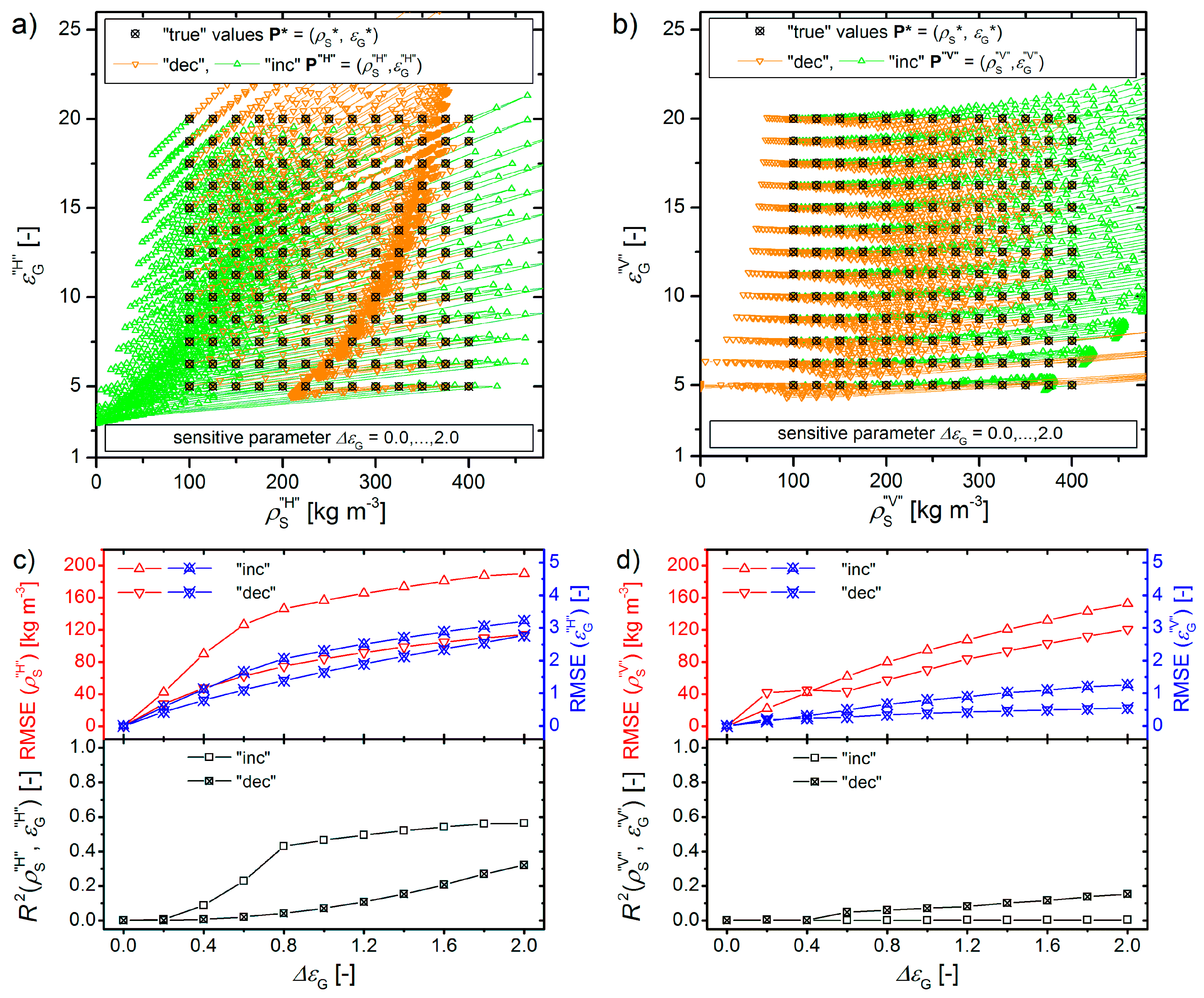
Figure 5a,b show the sensitivities of retrievals and , respectively, to expressing the -variability of ground permittivities (Equation (3)). As was the case in Section 4.1, this sensitivity analyses is performed over the two-dimensional space of “true” values (crossed black circles) for and with respective steps and . The two-dimensional retrieval space is spanned by the pairs achieved for scan sets simulated for each pair and -dependent ground permittivities . Thereby, the examined heterogeneity parameter involved in defined in Equation (3), is varied within in steps of to yield trajectories of retrieval pairs (colored connected symbols) originating from each . Furthermore, increasing (type = “inc.”) and decreasing (type = “dec.”) ground permittivity towards shallower nadir angles (increasing ) are considered with associated retrievals shown in Figure 5 with green up-triangles and orange down triangles, respectively. As is outlined in Section 3.3.2, and illustrated with the inset in the flowchart in Figure 3, “true” values are defined as averaged over the range of nadir angles considered for elevation scan sets .
Similarly to Figure 4, the transformation of the space of uncorrelated “true” values to the retrieval spaces depends significantly on the retrieval mode RM = “H” and “V”. This becomes obvious from the qualitatively different patterns of scatters of the respective retrievals and shown in Figure 5a,b. Furthermore, the transformations are considerably different for increasing (type = “inc.”) and decreasing (type = “dec.”) types of ground permittivity variability among footprints. However, in any case (RM = “H”, “V” and type = “inc.”, “dec.”), trajectories of retrieval pairs (colored connected symbols) are extensively stretched along the horizontal snow density axis, while their stretch along the vertical ground permittivity axis is relatively small. This observation suggests that generally, are significantly distorted by variable ground permittivity among footprints, while retrievals remain closely comparable with their respective “true” values .
Figure 5c,d present the respective qualitative picture of the retrievals’ distortion that is caused by , based on the retrieval pairs and , as shown in Figure 5a,b. The respective lower panels show retrievals’ coefficient of determination for . For uniform ground permittivities among footprints at () retrievals’ correlations are necessarily for RM = “H” and “V”. For RM = “H” (Figure 5c), retrievals’ correlation reaches for type = “inc.” and for type = “dec.” for , whereas for RM = “V” are smaller and almost zero for type = “inc.” The generally similar trend of higher correlation between for RM = “H” than “V” complements the findings that retrievals’ sensitivities with respect to the “geophysical noise” sources investigated in [39] is higher for RM = “H” than “V”. Similar to that shown in Figure 4c,d, the behavior of in Figure 5c,d (blue symbols) reveals that are only marginally distorted by for both RMs and types of . However, of snow density retrievals are noticeably large, even for the relatively small . For example, for and type = “inc.”, errors of retrievals reach (upward-pointing red triangles in Figure 5c) implying that are distorted so much that they become almost independent of their respective “true” values . This distortion also appears in the respective retrieval trajectories (Figure 5a,b), which are largely stretched along the horizontal snow density axes. This clearly indicates that retrievals are only realistic for small variability among ground permittivities of footprints at different .
The high sensitivities of retrievals to is seen as crucial for the practicability of the retrieval scheme. For radiometers operating in the “swath scanning” configuration, reliable retrievals are most likely limited to frozen ground conditions, for which footprint variability of ground permittivity is expected to be low. Furthermore, the present sensitivity analysis indicates the advantage of multi-angle measurements of overlapping footprint areas (for example SMOS [23]) over scan sets that are acquired with a “swath scanning” radiometer [42], which looks at different footprint areas at different nadir angles .
5. Experimental Retrievals
5.1. Multi-Angle Retrievals
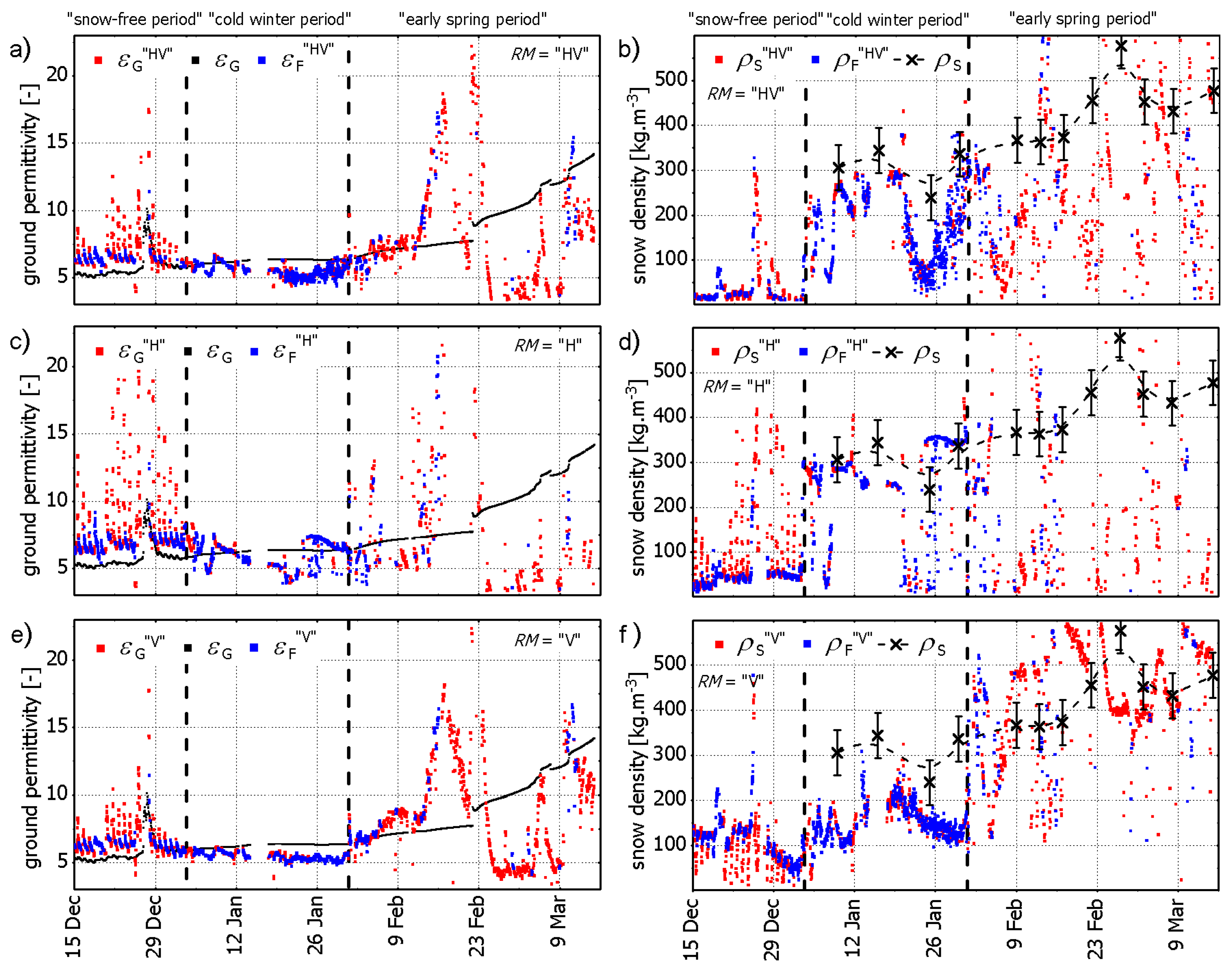
Figure 6 shows the multi-angle retrievals of snow bottom-layer mass density and ground permittivity for retrieval modes RM = “HV”, “H”, and “V” using elevation scan sets measured at . The presented period from 15 December 2016 to 15 March 2017 encompasses the “snow-free period”, “cold winter period”, and “early spring period”. The vertical dashed lines on 3 and 31, January indicate the onset of the dry snow cover present throughout the entire “cold winter period” and the beginning of the “early spring period” defined by the first occurrence of measurable amounts of liquid snow water (see Section 5.3 in [41] and Section 4.1 in the companion paper [40]), respectively. Concurrent in-situ measured ground permittivity (averaged over the two in-situ transects—the data as in Figure 2) and bottom-layer snow density . are shown with red markers in Figure 6.
During the “snow-free period”, retrievals for RM = “HV”, “H”, and “V” (Figure 6a,c,e) follow similar temporal patterns, exhibiting distinct diurnal spikes mostly during afternoons. The latter result from daily increases in air temperature (blue symbols in Figure 2d) above 0 °C, which, in turn, cause local thawing of the ground, and thus increased variability of ground permittivities among the footprint areas observed at (Figure 1). However, when compared to the spatially averaged in-situ references , offsets and diurnal deviations are slightly larger for (Figure 6c) than for retrievals (Figure 6e). This observation is consistent with simulated errors resulting from -dependent ground permittivities , as shown in Figure 5c,d. Higher uncertainties in retrievals as compared to are also expected from the higher angular sensitivity of when compared to as is shown in Figure 3b in [30] for the situation of a snow-free frozen ground. However, given the relatively large difference between the typical frozen and unfrozen ground permittivity values [47,48], retrievals, for all RMs, detect the ground freeze/thaw state reliably nonetheless.
With the beginning of the “cold winter period” and the concurrent first dry snow event on 3 January 2017, the daily fluctuations of in-situ and retrieved (Figure 6) disappear. This is due to thermal insulation of the developing dry snowpack [49,50], which keeps the ground homogeneously frozen even for short diurnal periods with (as is the case during the “cold winter period” after 19 January according to Figure 2d).
Multi-angle retrievals (Figure 6a) achieved for RM = “HV” as well as retrievals (Figure 6e) for RM = “V” follow the in-situ measured roughly until 12 February. However, with the beginning of the “early spring period” (31 January), and reveal increasing trends followed by severe over- and under-estimation of in-situ measurements after 12 February, which, given the typical permittivities of and for frozen and thawed ground [47,48], may even cause false classifications of ground freeze/thaw states. Similar observations are made for retrievals (Figure 6c). However, due to the limited number of physically reasonable retrievals, the corresponding temporal patterns are not as clear as for and shown in Figure 6a,e, respectively.
Snow density retrievals (Figure 6b) and (Figure 6d) throughout the “snow-free period” are in most cases , whereas a sudden jump to takes place on 3 January concurrently with the onset of dry snow, which defines the beginning of the “cold winter period”. The first occurrence of dry snow is best captured by the retrievals with RM = “H” (Figure 6d) and least distinctly by the retrievals when RM = “V” (Figure 6f). This experimental observation clearly demonstrates the capability of the investigated multi-angle retrieval [30] when used with the retrieval modes RM = “H” or “HV” to distinguish between absence and presence of dry snow above ground. Additionally, throughout the “cold winter period” with exclusively dry snow atop the homogeneously frozen ground, retrievals (Figure 6d) estimate in-situ measured snow bottom-layer density fairly accurately when considering their approximate uncertainty range of .
It is noteworthy that while detect the onset of snow cover over the site better than RM = “V”, the retrievals follow the pattern of in-situ measured temporal variations better than density retrievals when RM = “H”. Additionally, when comparing the population of the retrievals for RM = “V” and “H” during the “early spring period” shows that the number of physically meaningful retrieval pairs is considerably larger when using RM = “V” than when using RM = “H”. In summary, retrievals for both RM = “H” and “V” benefit and suffer from a number of the aforementioned advantages and disadvantages, respectively. Thus, performing analyses with RM = “HV”, which uses from both p = H and V in Equation (1), can yield more accurate results under certain circumstances (see Section E in [39]).
It can be seen that, simultaneously with the observed increasing deviations between retrieved and in-situ ground permittivities starting with the “early spring period”, retrievals also start diverging from in-situ references . The digression of -retrieval performance is observed for all of the RMs. This is mostly attributed to the occurrence of snow liquid water (Section 4.1) and/or variability in ground permittivity among footprints (Section 4.2) caused by local thawing of the ground surface layer. Both of these instances are “melting effects” that emerge during warm winter periods and are considered to be sources of “geophysical noise” in addition to those that are investigated in [39]. “Geophysical noise” associated with “melting effects” can either diminish retrieval performance or even lead to physically meaningless retrieval values . However, it is important to note that retrieval error analyses with respect to the aforementioned “melting effects” (Section 4.1 and Section 4.2) suggest . This is consistent with the better representation of the temporal pattern of in-situ by retrievals achieved for RM = “V” than for RM = “H”. Furthermore, simulated impacts of variability of ground permittivity among footprints revealed very strong displacements of the two-dimensional space of realistic “true” values to the retrieval space , as illustrated in Figure 5a,b.
Ultimately, during the “early spring period”, these “melting effects” lead to snow and ground states that are by no means adequately represented by the configuration (uniform dry snow and ground) of the emission model “LS-MEMLS” (Section 5.1 in [41] and in [30]) used in the retrieval scheme (Section 3.1). This results in the total lack of pattern similarity between retrieval pairs and corresponding in-situ references over the course of the “early spring period”. It should be noted that in each of the two earlier periods, we have only taken the most influential type of “geophysical noise” into consideration. In reality, retrieval disturbances are caused by the collective impact of all the “geophysical noise” discussed in Section 4 (snow liquid water and footprint-dependent ground permittivity) and in [39] (ground roughness, snow density variability).
The discussion above explains the degradation of multi-angular retrievals caused by “geophysical noise” associated with “melting effects”. The rest of this subsection explores conjunctions which cause a correlation between measurement-based retrievals and , and the potential use of the respective coefficients of determination to raise a “quality flag” that indicates limited retrieval performance. As demonstrated in Section 4, the coefficients of determination between retrievals are expected to be , given that the assumptions (homogeneous ground covered with single-layer dry snowpack) made in “LS-MEMLS” and employed in the retrieval scheme (Section 3.1) are fully consistent with the conditions of the footprint areas in elevation scan sets . However, departures from these assumptions result in correlated retrievals (), as is shown for the presence of moist snow (Figure 4) and ground permittivities that vary among footprints at of an elevation scan (Figure 5). Accordingly, we suggest utilizing retrieval correlations as a quality indicator to mark weakly correlated retrieval pairs () as “reliable”, and significantly correlated pairs () as “questionable”.
In order to investigate this potential opportunity, retrievals’ coefficients of determination are computed for any given time t in a 12-hour asymmetric sliding window based on time-series of retrieved from measured elevation scan sets . The choice of the length of the correlation time window is important as it should (i) be long enough to contain meaningful representative measurement statistics, and (ii) be short enough not to smear out critical temporal variations in the state of the snow-covered ground.
Figure 7a–d show pairs of histograms of for retrieval modes RM = “V” and “H”, respectively, for the period 15 December to 5 February covering the entire “cold winter period”, as well as parts of the “snow-free period” and “early spring period”. Figure 7a,c are for retrievals based on early “morning” (02:00–08:00) measurements, the time window in which the aforementioned retrieval assumptions (homogeneously frozen ground covered with dry snow) are best met. Figure 7b,d are for corresponding retrievals based on “afternoon” (12:00–18:00) measurements, the time window in which departures from assumptions made for the retrieval (due to “melting effects” that cause moist snow and varying ground permittivities among footprints as demonstrated in the companion paper [40]), as well as attendant retrieval distortions, are expected to be most prominent.
A comparison of the histograms in Figure 7a,b shows that for RM = “V” values, are generally lower when using “morning” measurements than when using “afternoon” measurements. This supports the view that when the snowpack is dry (for the “cold winter period”) or the ground is fully frozen (for both the “snow-free period” and “cold winter period”), retrievals mostly exhibit very low coefficients of determination. Additionally, a comparison of in Figure 7a,b with in Figure 7c,d shows considerably lower retrieval correlations when RM = “V” than when RM = “H”. This points to the better performance of the vertical polarization retrieval mode, the reason for which is shown in Figure 6 for the “snow-free period” and is discussed in Section 4 for the period with snow-covered ground.
Although Figure 8 shows the same retrievals as in Figure 6, retrievals for which the “quality flag” is raised based on increased correlation, are colored in red. For all retrieval modes, “quality flags” are determined based on correlations between retrievals performed with RM = “V” where the maximum threshold . The rationale for selecting correlations between V-mode retrievals is provided below, following examples of “quality flags” based on , which successfully improves the temporal pattern of in comparison to corresponding in-situ references .
As the first example of such improvements, employing the “quality flags” reliably identifies the short daily spikes of . retrieved during the “snow-free period” when the ground is fully frozen (Figure 8a,c,e). Retrievals also take advantage of obvious filtering benefits, meaning that large portions of obvious outliers are detected for the “snow-free period” (Figure 8b,d,f). As a second example, -based “quality flags” are successful during the “early spring period”, when snow and ground conditions become more complex, and thus, are no longer adequately represented by the emission model “LS—MEMLS” that is used in the retrieval scheme. As already mentioned, under such conditions retrieval errors are increased as the result of “geophysical noise” associated with “melting effects”. This is fully consistent with the clear increase in the number of “quality flags” raised (red data points in Figure 8) during the “early spring period” in comparison to corresponding incidents during the “cold winter period”. To be more specific, the “quality flag” is reliably raised (red data points in Figure 8) when retrievals during the “early spring period” severely over- or under-estimate in-situ references . However, after 12 February, some retrievals are not captured by the “quality flag” (blue data points in Figure 8) even though they largely deviate from in-situ averaged over the two transects (Figure 1). Figure 10 in Section 5.2 shows that some of these retrievals do indeed correspond well with in-situ permittivity measurements specific to some of the footprint areas at .
The use of between V-mode retrievals —rather than for example H-mode—to raise “quality flags” is due to both physical and practical considerations. The analysis of retrievals’ sensitivity with respect to snow liquid water (Section 4.1) has revealed that correlations between H-mode retrievals are so sensitive that even very small amounts of snow liquid water column can result in (Figure 4c). In contrast, corresponding coefficients of determination between V-mode retrievals (Figure 4d) remain significantly smaller. Likewise, are expected, even for small variability of ground permittivities among footprints, as demonstrated in the respective sensitivity analysis (Section 4.2). In general, retrievals achieved with RM = “V” are less prone than those with RM = “H” (and “HV”) to “geophysical noise”, originating from snow liquid water (Section 4.1), ground permittivities varying among footprints (Section 4.2), or those that are discussed in [39] (ground surface roughness and varying mass-density across the snowpack profile). Therefore, using “quality flags” based on correlations between H-mode (or HV-mode) retrievals leaves us with few un-flagged retrievals even for the “cold winter period” when they follow the in-situ references reasonably well as demonstrated in Figure 6. On the other hand, the experimentally-observed filtering benefits discussed above are clearly in favor of using the threshold based on V-mode retrievals as “quality flags”. Another advantage of using correlations between V-mode retrievals as “quality flags” is the distinct drop in the population of un-flagged retrievals with the beginning of the “early spring period”. This observation based on our measurements is seen as an additional method for detecting the time of the onset of moist snow and the beginning of the snow-melt-down season as a complement to the snow water content retrieval approach, as presented in the companion paper [40].
We here summarize the key points mentioned thus far regarding multi-angle retrievals for retrieval modes RM = “H”, “V”, and “HV”:
- RM = “V”: Performs best for retrievals compared to corresponding in-situ references ; provides a suitable retrieval “quality flag” based on the threshold of retrieval coefficients of determination. The criterion can detect the onset of the “early spring period” characterized by increased snow liquid water as demonstrated in [40].
- RM = “H”: Retrievals are most suited to detect the onset of dry snow cover over frozen ground. Retrievals are generally more distorted by “geophysical noise” associated with “melting effects”, and thus are much less “successful” during the “early spring period” compared to V-mode retrievals.
- RM = “HV”: Retrievals comprise features of both retrieval modes RM = “H” and “V”. It is suggested that RM = “HV” be used for snow density retrievals as it: (a) detects and distinguishes the onset of dry snow, (b) represents in-situ references , and (c) is less prone to instrumental uncertainties because it is based on twice as many measurements .
5.2. Single-Angle Retrieval
Multi-angle retrievals are derived from measured elevation scan sets . Accordingly, , as presented in Section 5.1, are necessarily “effective” parameter values that are representative of the entire area covered by all the footprints observed at the nadir angles (Figure 1) using the ELBARA-II radiometer in the “swath scanning” configuration [42]. Conversely, the single-angle retrievals shown here and achieved using the approach outlined in Section 3.2, represent snow densities and ground permittivities within individual footprint areas observed at . This is because retrieval pairs are derived solely from the two measurements and performed at a given . As a consequence, the value of the higher spatial resolution of single-angle retrievals as compared to multi-angle retrievals may come at the expense of higher retrieval uncertainties. However, it is worth investigating single-angle retrievals because they provide insight into spatial heterogeneities of the study-site, which, in turn, can support the interpretation of the multi-angle retrievals in terms of their distortion caused by, for instance, -dependent ground permittivities as a type of “geophysical noise” induced by “melting effects”.
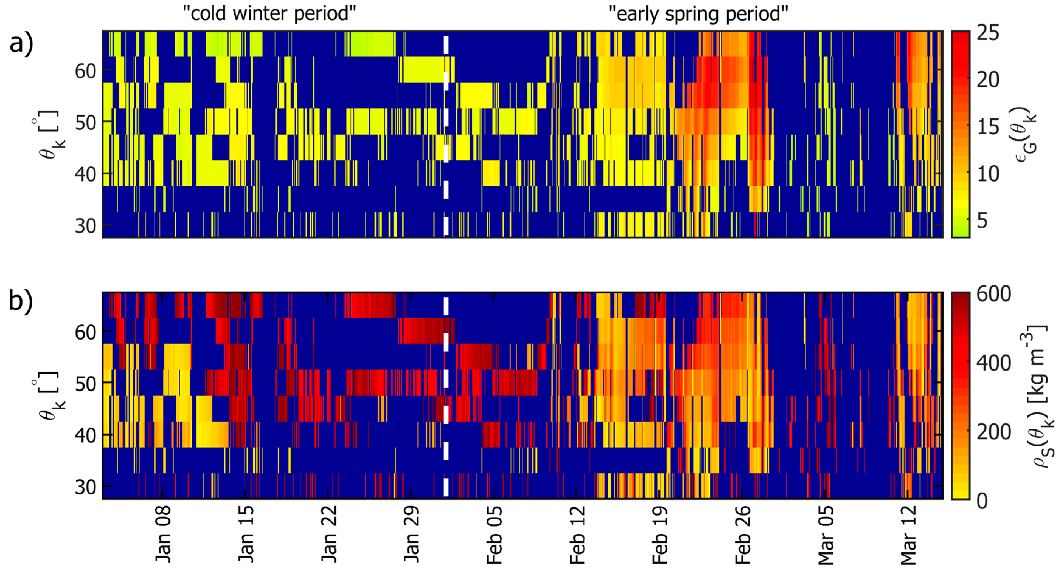
Figure 9a,b show color-coded single-angle ground permittivities and snow density retrievals , respectively. The dark blue pixels indicate failed retrievals, where the equation system (2) has no real solution for a pair (p = H, V) measured at . Nevertheless, generally throughout the measurement campaign and especially before the second half of the “early spring period” in March, the occurrence of physically meaningful single-angle retrievals is sufficient to estimate the temporal evolution of footprint-specific snow density and ground permittivity, as discussed subsequently.
Figure 9a indicates a frozen ground with for all footprint areas observed at up to around mid-February. After this date, the footprint areas observed at shallower nadir angles () show higher indicating faster thawing than in the footprint areas that are observed at steeper nadir angles (). The last time period with a statistically relevant number of “successful” single-angle retrievals (“successful” means that is a real solution of the equation system (2)) per elevation scan set comes after a period with few “successful” retrievals, roughly between 28 February and 10 March. This last period’s values indicate the continued trend of the ground’s thawing.
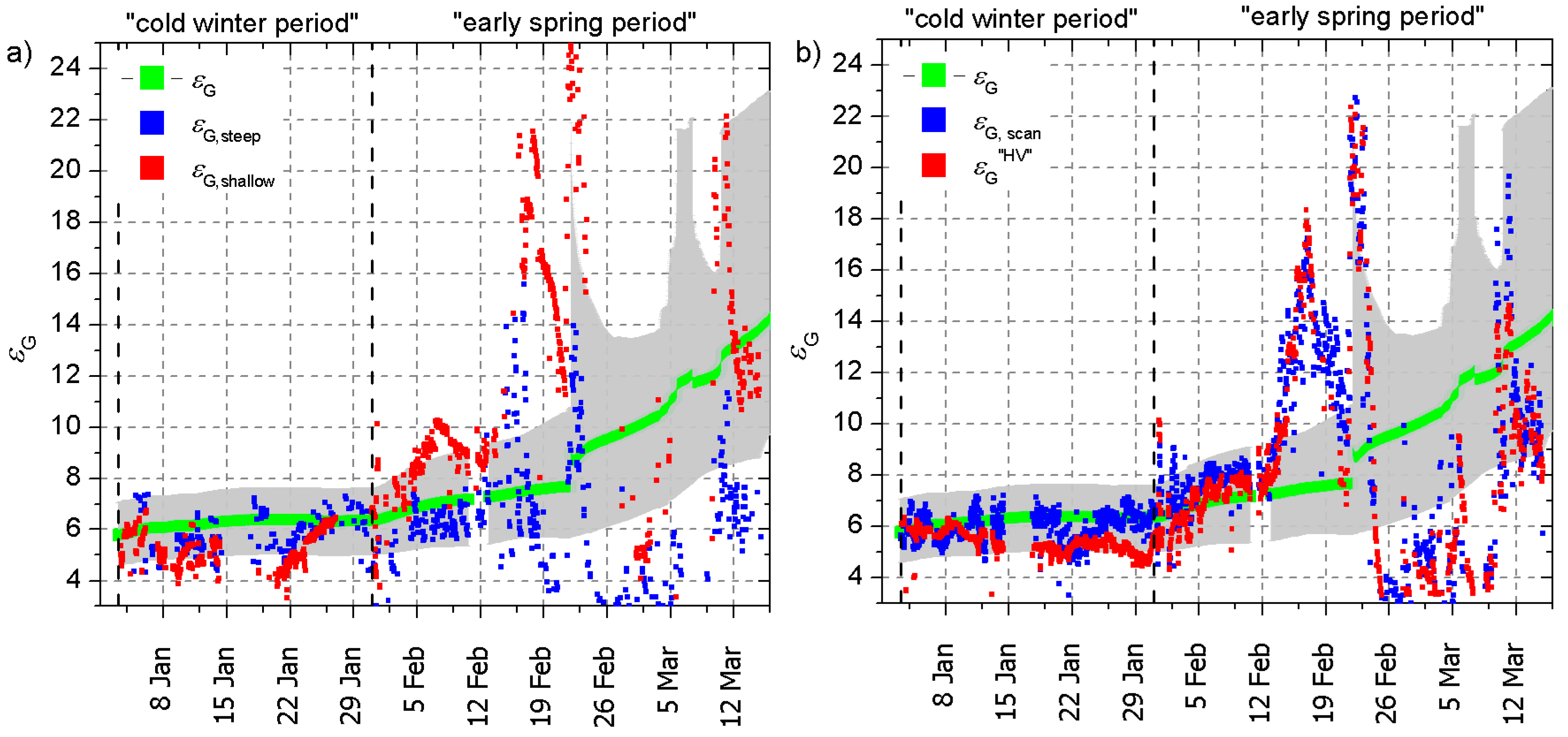
The differences between at different nadir angles observed in Figure 9a indicate spatial variability in ground permittivity among the footprint areas. Figure 10a shows the average of “successful” ground permittivity retrievals for (blue) and for (red) for the same time period as in Figure 9. In addition to the retrievals and , Figure 10a includes the references in green (same as in Figure 2a,b), representing the mean of all in-situ measurements that were performed along the two transects (Figure 1). The gray area shows their spread, representing the temporal evolution of ground permittivities’ spatial variability. Consequently, retrievals and that fall within, or in close proximity to the gray marked area are considered to be consistent with in-situ observations. An example of this takes place on 21 February (black dashed line in Figure 10a) where very high values are observed for , which are coincident with the high readings of the sensor d (Figure 2b) installed at the outer end of the in-situ transect 2. This suggests high ground permittivity of the shallow footprint observed at (Figure 1). However, the limited areal coverage of in-situ measured ground permittivities restricts our ability to claim with certainty whether the increased retrievals between 14 and 22 February are realistic or are otherwise caused by some kind of “geophysical noise”.
It is evident in Figure 10a that single-angle retrievals are very similar for all throughout the entire “cold winter period” (3–31 January), indicating a homogeneously deeply-frozen ground underneath the dry snowpack. However, it can be seen that, starting from 5 February, (red) are mostly greater than (blue). This again illustrates that the ground areas within shallower angle footprints start to thaw up sooner than ground areas within steeper angle footprints. Furthermore, the observed trend provides experimental evidence for the conclusion that is made in Section 4.2, that, given the employed “swath scanning” method, multi-angle retrievals perform best in comparison to in-situ for deeply frozen ground states. This is corroborated by the timing when differences between multi-angle retrievals and in-situ references grow (Figure 6) at the beginning of the “early spring period” (31 January) and the contemporaneous manifestation of the pronounced divergence of averaged single-angle retrievals and (Figure 10a), which indicate an increased variability among footprint permittivities.
Figure 10b shows single-angle retrievals (blue) averaged over the full range of azimuth angles considered in the multi-angle retrievals achieved with RM = “HV” and shown in red (the same as shown in Figure 6a). It can be seen that both (blue) and (red) estimate ground permittivities very similarly. This is because of the same representative ground area of both retrieval types corresponding to the total area that is covered by all of the footprints observed at .
It is noteworthy that through the “snow-free period” (not shown here), single-angle retrievals always have very low values (). They also detect the onset of the snow cover on 3 January by a marked increase to . Figure 9b shows the color-coded values of single-angle retrievals of snow mass-density over the snow-covered period from 3 January to 15 March. Single-angle retrievals , averaged over the entire nadir angle range , generally yield higher values than multi-angle retrievals . Furthermore, the shift of retrieval values in Figure 9b from (15 January–12 February) to (13–28 February) and then to (1–10 March) is similar to the over- and under-estimated multi-angle retrievals in Figure 6, which show that retrievals are heavily influenced by snowpack wetness and increased spatial heterogeneities. This matches with the synthetic sensitivity analysis results in Section 4.
Comparing Figure 9a,b reveals that the relative angular scatter of single-angle retrievals in the first half of January are more pronounced than the scatter of corresponding single-angle retrievals . This is because the ground beneath the dry snow is the major contributor to the footprint emission . With the ground being totally frozen in the “cold winter period”, its emission is relatively stable and similar over the entire observed footprint area. Thus, -variability of evanesce during the “cold winter period”. However, -variability of is most apparent during approximately the first 10 days of the “cold winter period”, starting with the first snowfall. This is because it takes time and more precipitation until the newly-formed snowpack becomes spatially homogeneous and thick enough to avoid single-angle retrievals given that they are affected by, for example, coherent effects that are not considered in the emission model “LS—MEMELS”. Therefore, for all have similar and stable values roughly after 13 January until the end of the “cold winter period” on 31 January.
Just as is the case for the ground permittivity retrievals , the -variability of increases with the beginning of the “early spring period” as a result of “melting effects” that are associated with increasing time-integrated heat-input to the snow covered ground. When comparing the color graphs in Figure 9a,b for the two consecutive weeks between 12 and 26 February reveals that retrievals start showing signs of heterogeneities among footprints sooner than . This is explained by the thermal insulation of the snowpack, which delays local thawing of the ground as compared to the faster thawing of upper parts of the snowpack. Towards the end of the “early spring period” (28 February–15 March), with its demonstrated high amounts of snow liquid water [40], the number of “successful” single-angle retrievals drops significantly. Nevertheless, the few remaining legitimate retrievals, which occur mostly during short-term freezing periods, can still provide a picture of snow and ground status. However, for the period 28 February–15 March, the amount of extractable information from retrievals is minimized down to the presence or absence of snow and the steady thaw-up of the ground.
6. Summary and Conclusions
The experimental L-band radiometry data, from the winter 2016/2017 campaign at the Davos-Laret Remote Sensing Field Laboratory, was successfully used to perform multi-angle and single-angle retrievals for the “snow-free period”, “cold winter period”, and “early spring period”. On the one hand, the content of the present paper can be seen as an additional experimental validation of the snow density and ground permittivity retrieval approach proposed in [30] and first validated by [31]. It has also been shown that the single-angle experimental retrievals , which were mainly performed to study the impact of spatially variable ground permittivity on multi-angle retrievals’ performance, perform reasonably well, and, once averaged over nadir angles , yield very similar results to the multi-angle retrievals . On the other hand, this work extends the analysis of retrieval approaches with respect to the sensitivity of multi-angle retrievals to “melting effects” that occur in the snowpack and the underlying ground. To demonstrate this, synthetic sensitivity analyses were conducted to study the impacts of “melting effects”, in the form of two types of “geophysical noise” (snow liquid water column and footprint-dependent ground permittivity ), on the retrievals . It should be recalled that the aforementioned “geophysical noise” sources are essentially caused by digressions from the assumptions of a dry snowpack over a homogeneous ground in the retrieval algorithm based on “LS—MEMLS”. It has been shown that increased snow liquid water, which—as demonstrated in the companion paper [40]—appears with the beginning of the “early spring period”, causes noticeable disturbances in , and even more in retrievals. Also, it has been demonstrated that footprint-dependent ground permittivities, as another source of “geophysical noise” due to “melting effects”, can cause significant disturbances in retrievals . Such disturbances, caused by the aforementioned “geophysical noise”, result in noticeably high correlations between retrievals . However, these heterogeneities are only relevant when radiometry is done in the “swath scanning” mode and mainly for the “early spring period” when the ground state gradually changes from a homogeneously frozen state to locally thawed. As an improvement to the first experimental two-parameter retrieval in [31], it is suggested that the coefficients of determination can be used as a “quality flag” for retrievals such that those with low are considered as acceptable, while retrievals with are flagged as potentially distorted by “geophysical noise” associated with “melting effects”.
In both of the aforementioned analyses, and according to the presented retrieval errors, retrievals are more prone than retrievals to “melting effects” (causing “geophysical noise”, i.e., snow liquid water and footprint-dependent ground permittivity). Additionally, retrievals with RM = “V” are generally less influenced by such “geophysical noise” than RM = “H”. This finding corroborates with the results of the earlier sensitivity analysis [39], which was dedicated to the investigation of the impact of ground roughness and varying mass-density across the snow profile, as other potential types of “geophysical noise”, on .
The comparison of the experimental retrievals , derived from elevation scan sets of tower-based “swath scanning” L-band radiometer measurements, with their in-situ measured counterparts , indicate that the most consistent retrievals are obtained for the “snow-free period” and “cold winter period” when “geophysical noise” is at its minimum and ground-snow emission system properties best match the retrieval algorithm assumptions of uniform dry snowpack over a homogenous ground. Furthermore, using the aforementioned “quality flag” significantly improves the degree of harmony between retrievals and in-situ data by successfully flagging inaccurate or unreal retrievals.
Our results also suggest the use of the retrieval modes RM = “V” for and RM = “HV” for retrievals. It has been shown that the latter takes advantage of RM = “H” in the detection of the presence of dry snow and its mass density, while RM = “V” is able to better capture the temporal variations of snow mass-density. Finally, it is suggested that the considerable drop in the population density of un-flagged retrievals can be used as an indicator of the start of the “early spring period”. This is a method that may be considered in addition to the retrieval of snow liquid water as is proposed in the companion paper [40].
When considering its promising performance, especially for “snow-free period” and “cold winter period”, as demonstrated in this paper and in [31], together with the introduction of “quality flags”, we suggest to test the presented two-parameter retrieval with space-borne L-band radiometry data, e.g., from SMOS, measured over northern latitudes. If successful, and can be implemented as new data products in a future version of SMOS processor, resulting in a further step towards the full exploitation of satellite L-band radiometry data.
Acknowledgments
This paper was supported in part by the Swiss National Science Foundation under Grant 200021L_156111 /1, and in part by ESA within the framework of ESA’s SMOS ‘Expert Support Laboratory’ (ESL) for Level 2. We would like to express our appreciation to Christian Mätzler for his valuable scientific inputs to the research presented. We also acknowledge the Forschungszentrum Jülich (FZJ) for providing the ELBARA-II radiometer funded via the German Helmholtz Association TERrestrial ENvironmental Observatories (TERENO) infrastructure project. We would also like to thank Matthias Jaggi from the WSL Institute for Snow and Avalanche Research SLF for conducting in-situ snow characterization measurements, Curtis Gautschi for editing the manuscript, and Manfred Stähli for his helpful comments.
Author Contributions
Mike Schwank and Reza Naderpour conceived, designed, and performed the experiments in equal shares. Likewise, they contributed equally to the data analyses and the writing of the manuscript.
Conflicts of Interest
The authors declare no conflict of interest.
References
- Malenovský, Z.; Rott, H.; Cihlar, J.; Schaepman, M.E.; García-Santos, G.; Fernandes, R.; Berger, M. Sentinels for science: Potential of Sentinel-1, -2, and -3 missions for scientific observations of ocean, cryosphere, and land. Remote Sens. Environ. 2012, 120, 91–101. [Google Scholar] [CrossRef]
- Hollmann, R.; Merchant, C.J.; Saunders, R.; Downy, C.; Buchwitz, M.; Cazenave, A.; Chuvieco, E.; Defourny, P.; de Leeuw, G.; Forsberg, R.; et al. The ESA Climate Change Initiative: Satellite Data Records for Essential Climate Variables. Bull. Am. Meteorol. Soc. 2013, 94, 1541–1552. [Google Scholar] [CrossRef] [Green Version]
- Mätzler, C. Applications of SMOS over terrestrial ice and snow. In Proceedings of the 3rd SMOS Workshop, DLR, Oberpfaffenhofen, Germany, 10–12 December 2001. [Google Scholar]
- Pulliainen, J.; Hallikainen, M. Retrieval of Regional Snow Water Equivalent from Space-Borne Passive Microwave Observations. Remote Sens. Environ. 2001, 75, 76–85. [Google Scholar] [CrossRef]
- Leduc-Leballeur, M.; Picard, G.; Mialon, A.; Arnaud, L.; Lefebvre, E.; Possenti, P.; Kerr, Y. Modeling L-Band Brightness Temperature at Dome C in Antarctica and Comparison With SMOS Observations. IEEE Trans. Geosci. Remote Sens. 2015, 53, 4022–4032. [Google Scholar] [CrossRef]
- Owe, M.; Jeu, R.d.; Walker, J. A methodology for surface soil moisture and vegetation optical depth retrieval using the microwave polarization difference index. IEEE Trans. Geosci. Remote Sens. 2001, 39, 1643–1654. [Google Scholar] [CrossRef]
- Meesters, A.G.C.A.; Jeu, R.A.M.D.; Owe, M. Analytical derivation of the vegetation optical depth from the microwave polarization difference index. IEEE Geosci. Remote Sens. Lett. 2005, 2, 121–123. [Google Scholar] [CrossRef]
- Kim, Y.; Kimball, J.S.; McDonald, K.C.; Glassy, J. Developing a Global Data Record of Daily Landscape Freeze/Thaw Status Using Satellite Passive Microwave Remote Sensing. IEEE Trans. Geosci. Remote Sens. 2011, 49, 949–960. [Google Scholar] [CrossRef]
- Rautiainen, K.; Parkkinen, T.; Lemmetyinen, J.; Schwank, M.; Wiesmann, A.; Ikonen, J.; Derksen, C.; Davydov, S.; Davydova, A.; Boike, J.; et al. SMOS prototype algorithm for detecting autumn soil freezing. Remote Sens. Environ. 2016, 180, 346–360. [Google Scholar] [CrossRef]
- Roy, A.; Toose, P.; Williamson, M.; Rowlandson, T.; Derksen, C.; Royer, A.; Berg, A.A.; Lemmetyinen, J.; Arnold, L. Response of L-Band brightness temperatures to freeze/thaw and snow dynamics in a prairie environment from ground-based radiometer measurements. Remote Sens. Environ. 2017, 191, 67–80. [Google Scholar] [CrossRef]
- Njoku, E.G.; Entekhabi, D. Passive microwave remote sensing of soil moisture. J. Hydrol. 1996, 184, 101–129. [Google Scholar] [CrossRef]
- Kerr, Y.; Waldteufel, P.; Wigneron, J.-P.; Martinuzzi, J.-M.; Font, J.; Berger, M. Soil moisture retrieval from space: The soil moisture and ocean salinity (SMOS) mission. IEEE Trans. Geosci. Remote Sens. 2001, 39, 1729–1735. [Google Scholar] [CrossRef]
- Njoku, E.G.; Jackson, T.J.; Lakshmi, V.; Chan, T.K.; Nghiem, S.V. Soil moisture retrieval from AMSR-E. IEEE Trans. Geosci. Remote Sens. 2003, 41, 215–229. [Google Scholar] [CrossRef]
- Melaas, E.K.; Richardson, A.D.; Friedl, M.A.; Dragoni, D.; Gough, C.M.; Herbst, M.; Montagnani, L.; Moors, E. Using FLUXNET data to improve models of springtime vegetation activity onset in forest ecosystems. Agric. For. Meteorol. 2013, 171–172, 46–56. [Google Scholar] [CrossRef]
- Xu, L.; Myneni, R.B.; Chapin, F.S., III; Callaghan, T.V.; Pinzon, J.E.; Tucker, C.J.; Zhu, Z.; Bi, J.; Ciais, P.; Tømmervik, H.; et al. Temperature and vegetation seasonality diminishment over northern lands. Nat. Clim. Chang. Lett. 2013, 3, 581–586. [Google Scholar] [CrossRef] [Green Version]
- Kim, Y.; Kimball, J.S.; Zhang, K.; McDonald, K.C. Satellite detection of increasing Northern Hemisphere non-frozen seasons from 1979 to 2008: Implications for regional vegetation growth. Remote Sens. Environ. 2012, 121, 472–487. [Google Scholar] [CrossRef]
- Fletcher, C.G.; Zhao, H.; Kushner, P.J.; Fernandes, R. Using models and satellite observations to evaluate the strength of snow albedo feedback. J. Geophys. Res. Atmos. 2012, 117. [Google Scholar] [CrossRef]
- Gouttevin, I.; Menegoz, M.; Dominé, F.; Krinner, G.; Koven, C.; Ciais, P.; Tarnocai, C.; Boike, J. How the insulating properties of snow affect soil carbon distribution in the continental pan-Arctic area. J. Geophys. Res. Biogeosci. 2012, 117. [Google Scholar] [CrossRef] [Green Version]
- Yang, D.; Robinson, D.; Zhao, Y.; Estilow, T.; Ye, B. Streamflow response to seasonal snow cover extent changes in large Siberian watersheds. J. Geophys. Res. Atmos. 2003, 108, 1–14. [Google Scholar] [CrossRef]
- Barnett, T.P.; Adam, J.C.; Lettenmaier, D.P. Potential impacts of a warming climate on water availability in snow-dominated regions. Nature 2005, 438, 303–309. [Google Scholar] [CrossRef] [PubMed]
- Papa, F.; Prigent, C.; Rossow, W.B. Ob’ River flood inundations from satellite observations: A relationship with winter snow parameters and river runoff. J. Geophys. Res. Atmos. 2007, 112. [Google Scholar] [CrossRef]
- Stewart, I.T. Changes in snowpack and snowmelt runoff for key mountain regions. Hydrol. Process. 2009, 23, 78–94. [Google Scholar] [CrossRef]
- Kerr, Y.H.; Waldteufel, P.; Wigneron, J.-P.; Delwart, S.; Cabot, F.; Boutin, J.; Escorihuela, M.-J.; Font, J.; Reul, N.; Gruhier, C.; et al. The SMOS mission: New tool for monitoring key elements of the global water cycle. Proc. IEEE 2010, 98, 666–687. [Google Scholar] [CrossRef] [Green Version]
- Mecklenburg, S.; Drusch, M.; Kerr, Y.H.; Font, J.; Martin-Neira, M.; Delwart, S.; Buenadicha, G.; Reul, N.; Daganzo-Eusebio, E.; Oliva, R.; et al. ESA’s Soil Moisture and Ocean Salinity Mission: Mission Performance and Operations. IEEE Trans. Geosci. Remote Sens. 2012, 50, 1354–1366. [Google Scholar] [CrossRef] [Green Version]
- Entekhabi, D.; Njoku, E.G.; O’Neill, P.E.; Kellogg, K.H.; Crow, W.T.; Edelstein, W.N.; Entin, J.K.; Goodman, S.D.; Jackson, T.J.; Johnson, J.; et al. The Soil Moisture Active Passive (SMAP) Mission. Proc. IEEE 2010, 98, 704–716. [Google Scholar] [CrossRef]
- Armstrong, R.L.; Brodzik, M.J. Recent northern hemisphere snow extent: A comparison of data derived from visible and microwave satellite sensors. Geophys. Res. Lett. 2001, 28, 3673–3676. [Google Scholar] [CrossRef]
- Dozier, J. Spectral signature of alpine snow cover from the landsat thematic mapper. Remote Sens. Environ. 1989, 28, 9–22. [Google Scholar] [CrossRef]
- Winther, J.G.; Gerland, S.; Ørbæk, J.; Ivanov, B.; Blanco, A.; Boike, J. Spectral reflectance of melting snow in a high Arctic watershed on Svalbard: Some implications for optical satellite remote sensing studies. Hydrol. Process. 1999, 13, 2033–2049. [Google Scholar] [CrossRef]
- Schwank, M.; Rautiainen, K.; Mätzler, C.; Stähli, M.; Lemmetyinen, J.; Pulliainen, J.; Vehviläinen, J.; Kontu, A.; Ikonen, J.; Ménard, C.B.; et al. Model for microwave emission of a snow-covered ground with focus on L band. Remote Sens. Environ. 2014, 154, 180–191. [Google Scholar] [CrossRef]
- Schwank, M.; Matzler, C.; Wiesmann, A.; Wegmuller, U.; Pulliainen, J.; Lemmetyinen, J.; Rautiainen, K.; Derksen, C.; Toose, P.; Drusch, M. Snow Density and Ground Permittivity Retrieved from L-Band Radiometry: A Synthetic Analysis. IEEE J. Sel. Top. Appl. Earth Obs. Remote Sens. 2015, 8, 3833–3845. [Google Scholar] [CrossRef]
- Lemmetyinen, J.; Schwank, M.; Rautiainen, K.; Kontu, A.; Parkkinen, T.; Mätzler, C.; Wiesmann, A.; Wegmüller, U.; Derksen, C.; Toose, P.; et al. Snow density and ground permittivity retrieved from L-band radiometry: Application to experimental data. Remote Sens. Environ. 2016, 180, 377–391. [Google Scholar] [CrossRef]
- Shi, J.; Dozier, J. Estimation of Snow Water Equivalence Using SIR-C/X-SAR, Part I: Inferring Snow Density and Subsurface Properties. IEEE Trans. Geosci. Remote Sens. 2000, 38, 2465–2473. [Google Scholar]
- Snehmani; Venkataraman, G.; Nigam, A.K.; Singh, G. Development of an inversion algorithm for dry snow density estimation and its application with ENVISAT-ASAR dual co-polarization data. Geocarto Int. 2010, 25, 597–616. [Google Scholar] [CrossRef]
- Thakur, P.K.; Aggarwal, S.P.; Garg, P.K.; Garg, R.D.; Mani, S.; Pandit, A.; Kumar, S. Snow physical parameters estimation using space-based Synthetic Aperture Radar. Geocarto Int. 2012, 27, 263–288. [Google Scholar] [CrossRef]
- Oh, Y.; Sarabandi, K.; Ulaby, F.T. An empirical model and an inversion technique for radar scattering from bare soil surfaces. IEEE Trans. Geosci. Remote Sens. 1992, 30, 370–381. [Google Scholar] [CrossRef]
- Shi, J.; Wang, J.; Hsu, A.Y.; O’Neill, P.E.; Engman, E.T. Estimation of Bare Surface Soil Moisture and Surface Roughness Parameter Using L-band SAR Image Data. IEEE Trans. Geosci. Remote Sens. 1997, 35, 1254–1266. [Google Scholar]
- Wiesmann, A.; Mätzler, C. Microwave emission model of layered snowpacks. Remote Sens. Environ. 1999, 70, 307–316. [Google Scholar] [CrossRef]
- Wigneron, J.-P.; Kerr, Y.; Waldteufel, P.; Saleh, K.; Escorihuela, M.-J.; Richaume, P.; Ferrazzoli, P.; de Rosnay, P.; Gurney, R.; Calvet, J.-C.; et al. L-band microwave emission of the biosphere (L-MEB) model: Description and calibration against experimental data sets over crop fields. Remote Sens. Environ. 2007, 107, 639–655. [Google Scholar] [CrossRef]
- Naderpour, R.; Schwank, M.; Mätzler, C.; Lemmetyinen, J.; Steffen, K. Snow Density and Ground Permittivity Retrieved From L-Band Radiometry: A Retrieval Sensitivity Analysis. IEEE J. Sel. Top. Appl. Earth Obs. Remote Sens. 2017, 10, 3148–3161. [Google Scholar] [CrossRef]
- Naderpour, R.; Schwank, M. Snow Wetness Retrieved from L-Band Radiometry. Remote Sens. 2018, 10, 359. [Google Scholar]
- Naderpour, R.; Schwank, M.; Mätzler, C. Davos-Laret Remote Sensing Field Laboratory: 2016/2017 Winter Season L-Band Measurements Data-Processing and Analysis. Remote Sens. 2017, 9, 1185. [Google Scholar] [CrossRef]
- Chang, A.; Rango, A.; Shiue, J. Remote sensing of snow properties by passive microwave. Microwave Remote Sens. Snowpack Prop. 1980, 169. Available online: https://ntrs.nasa.gov/search.jsp?R=19810010994. (accessed on 24 February 2018).
- Moeser, D.; Morsdorf, F.; Jonas, T. Novel forest structure metrics from airborne LiDAR data for improved snow interception estimation. Agric. For. Meteorol. 2015, 208, 40–49. [Google Scholar] [CrossRef]
- Bogena, H.R.; Huisman, J.A.; Schilling, B.; Weuthen, A.; Vereecken, H. Effective calibration of low-cost soil water content sensors. Sensors 2017, 17, 208. [Google Scholar] [CrossRef] [PubMed]
- Schwank, M.; Wiesmann, A.; Werner, C.; Mätzler, C.; Weber, D.; Murk, A.; Völksch, I.; Wegmüller, U. ELBARA II, An L-Band Radiometer System for Soil Moisture Research. Sensors 2010, 10, 584–612. [Google Scholar] [CrossRef] [PubMed]
- Schwank, M.; Wigneron, J.P.; Lopez-Baeza, E.; Völksch, I.; Mätzler, C.; Kerr, Y. L-Band Radiative Properties of Vine Vegetation at the SMOS Cal/Val Site MELBEX III. IEEE Trans. Geosci. Remote Sens. 2012, 50, 1587–1601. [Google Scholar] [CrossRef] [Green Version]
- Or, D.; Wraith, J.M. Temperature effects on soil bulk dielectric permittivity measured by time domain reflectometry: A physical model. Water Resour. Res. 1999, 35, 371–383. [Google Scholar] [CrossRef]
- Mironov, V.; Lukin, Y.I. A Physical Model of Dielectric Spectra of Thawed and Frozen Bentonitic Clay within the Frequency Range from 1 to 15 GHz. Russ. Phys. J. 2011, 53, 956–963. [Google Scholar] [CrossRef]
- Bernier, M.; Fortin, J.P.; Gauthier, Y.; Gauthier, R.; Roy, R.; Vincent, P. Determination of snow water equivalent using RADARSAT SAR data in eastern Canada. Hydrol. Process. 1999, 13, 3041–3051. [Google Scholar] [CrossRef]
- Ishikawa, M. Thermal regimes at the snow–ground interface and their implications for permafrost investigation. Geomorphology 2003, 52, 105–120. [Google Scholar] [CrossRef]
Figure 1.
Diagram of the footprint areas and the location of the in-situ sensors. ETH L-band Radiometer-II (ELBARA-II) was mounted atop an 8-m tower indicated by the hollow black square.
Figure 1.
Diagram of the footprint areas and the location of the in-situ sensors. ETH L-band Radiometer-II (ELBARA-II) was mounted atop an 8-m tower indicated by the hollow black square.
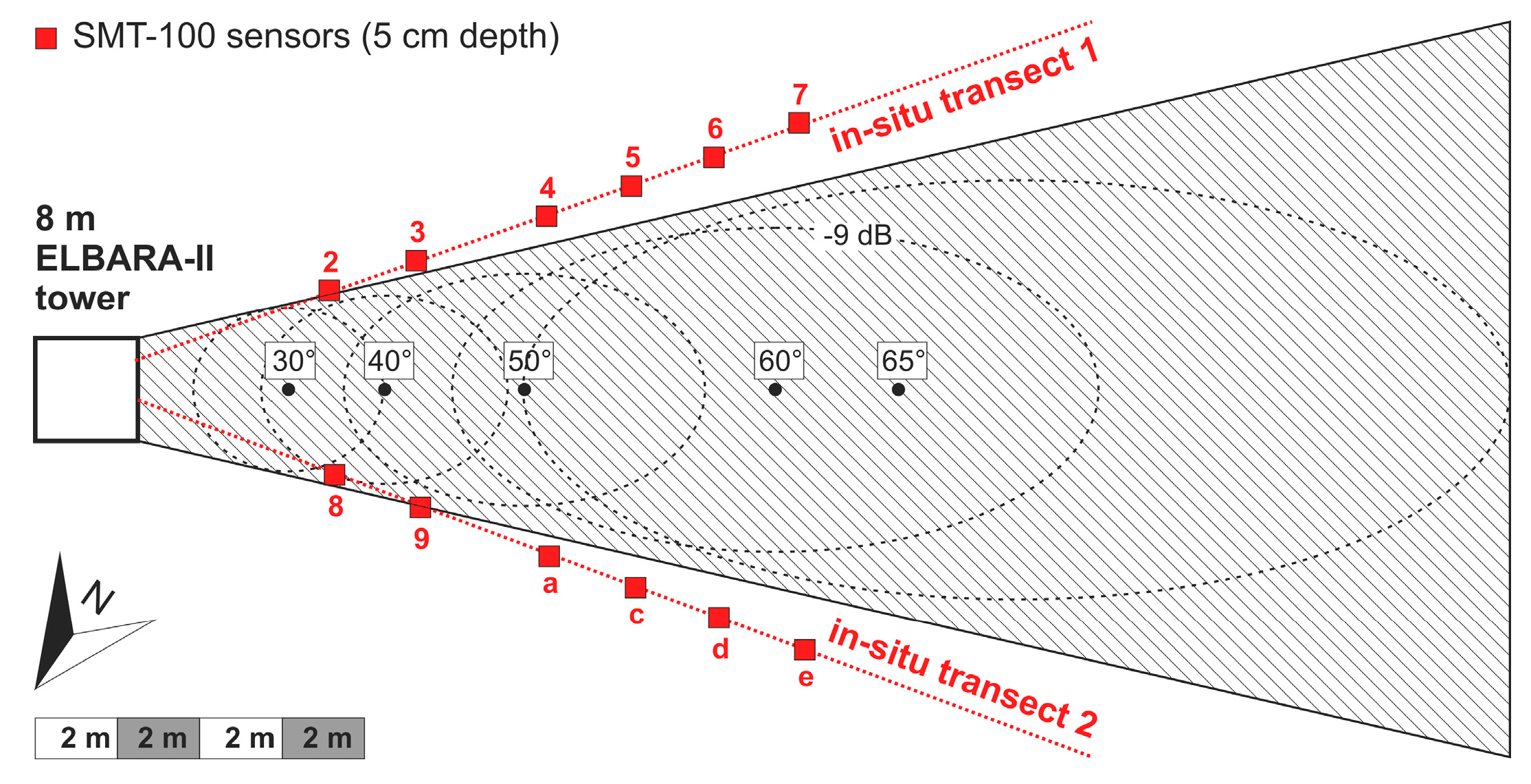
Figure 2.
Panels (a,b) show the time series of in-situ measured ground permittivities along transects 1 and 2 (shown in Figure 1), respectively. In panels (a,b), red indicates ground permittivitiy values resulting from averaging all 12 in-situ sensor readings. Panel (c) shows the average ground temperature measured by the 12 SMT-100 sensors. Panel (d) indicates temperatures , , and measured by ELBARA-II’s PT-100 temperature sensor and SMT-100 sensors placed 15 cm and 50 cm above ground, respectively. and show either air or snow temperatures depending on the snow height at the time of measurement. Panel (e) shows precipitation (both rain and snow). Panel (f) shows mass-density of the lowest 10 cm of the snowpack, as measured in-situ with a manual density cutter.

Figure 3.
Flowchart of the modeling approach used to infer sensitivities of retrieval pairs to “melting effects” such as: (a) snow liquid-water, and (b) spatial heterogeneity of ground permittivity.
Figure 3.
Flowchart of the modeling approach used to infer sensitivities of retrieval pairs to “melting effects” such as: (a) snow liquid-water, and (b) spatial heterogeneity of ground permittivity.

Figure 4.
Scatterplots of retrieval pairs (orange squares) for RM = “H” (panel (a)) and “V” (panel (b)) simulated for the two-dimensional space of “true” values (crossed black circles). For each snow liquid water column (the studied sensitive parameter) is varied within the range in steps of . Panels (c,d) show Root Mean Square Errors (solid blue dots), (open red dots) and retrievals’ coefficients of determination caused by .
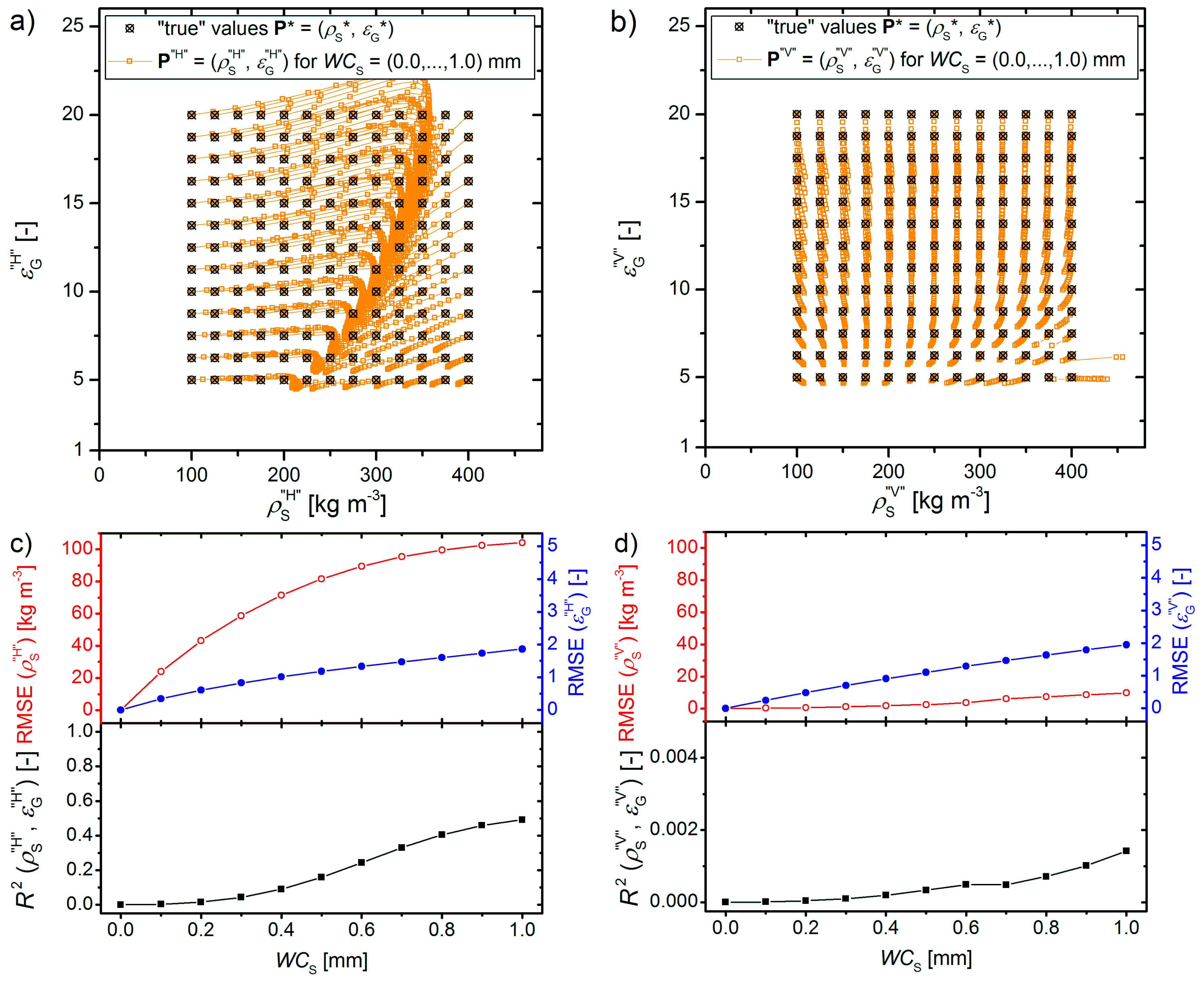
Figure 5.
Scatterplots of retrieval pairs for RM = “H” (panel (a)) and “V” (panel (b)) for “true” values (crossed black circles) and . For each the sensitive parameter in question is varied within (in steps of ). expresses -dependent ground permittivities ; “true” are defined as (averaging over ). Retrieval sensitivities to increasing (type = “inc.”, green) and decreasing (type = “dec.”, orange) are shown. Panels (c) and (d) show (blue), (red), and retrievals’ coefficients of determination (black) caused by .

Figure 6.
Multi-angle two-parameter retrievals for the time period 15 December, 2016–15 March, 2017. Panels (a,b) show the time series of and , respectively. Panels (c,d) and (e,f) show corresponding and for RM = “H” and “V”, respectively. Red markers show in-situ measured bottom-layer snow density and ground permittivity (same data as shown in Figure 2). The vertical dashed lines delimit the “snow-free period” (before 3 January), the “cold winter period” (3–31 January), and the “early spring period” (after 31 January).
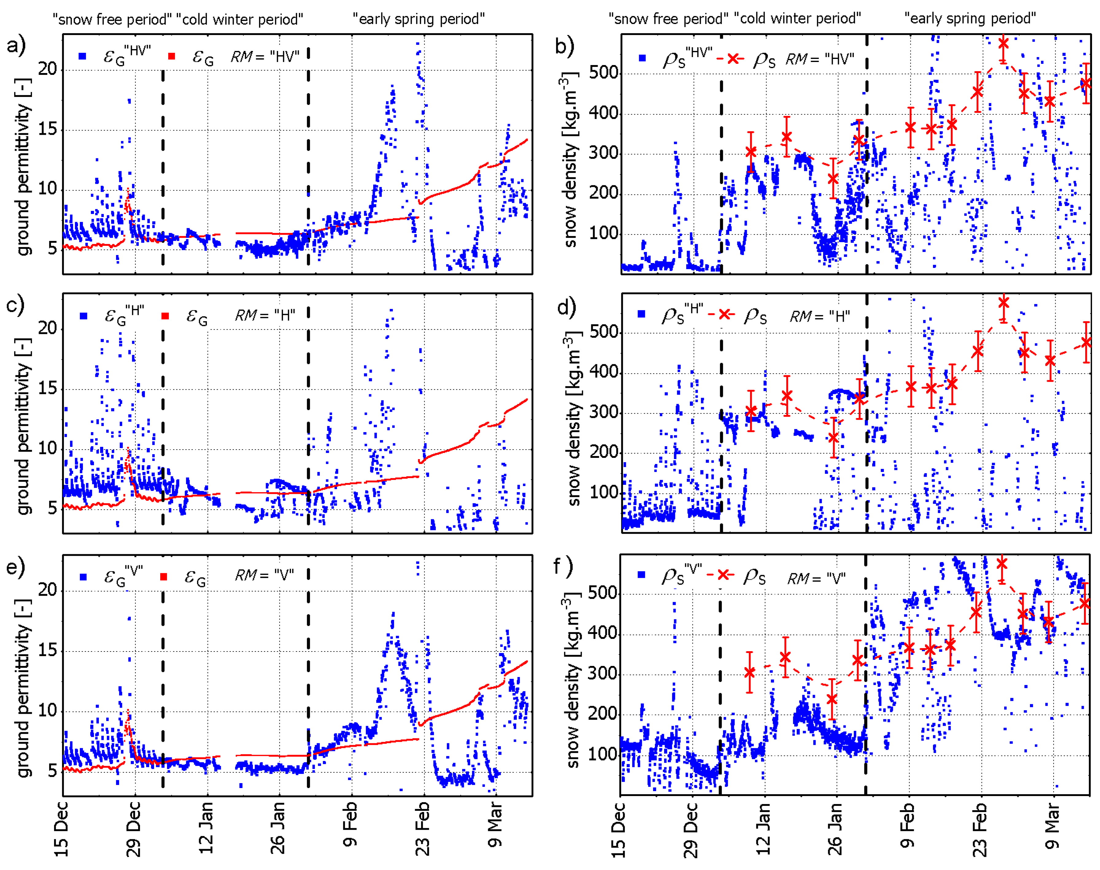
Figure 7.
Histograms of coefficients of determination for RM = “V” (a,b) and RM = “H” (c,d) of the retrieval pairs computed based on a sliding 12-h time window between 15 December, 2016 and 5 February, 2017. (a,c) are derived from “morning” (2:00–8:00) measurements, (b,d) are derived from “afternoon” (12:00–18:00) measurements.
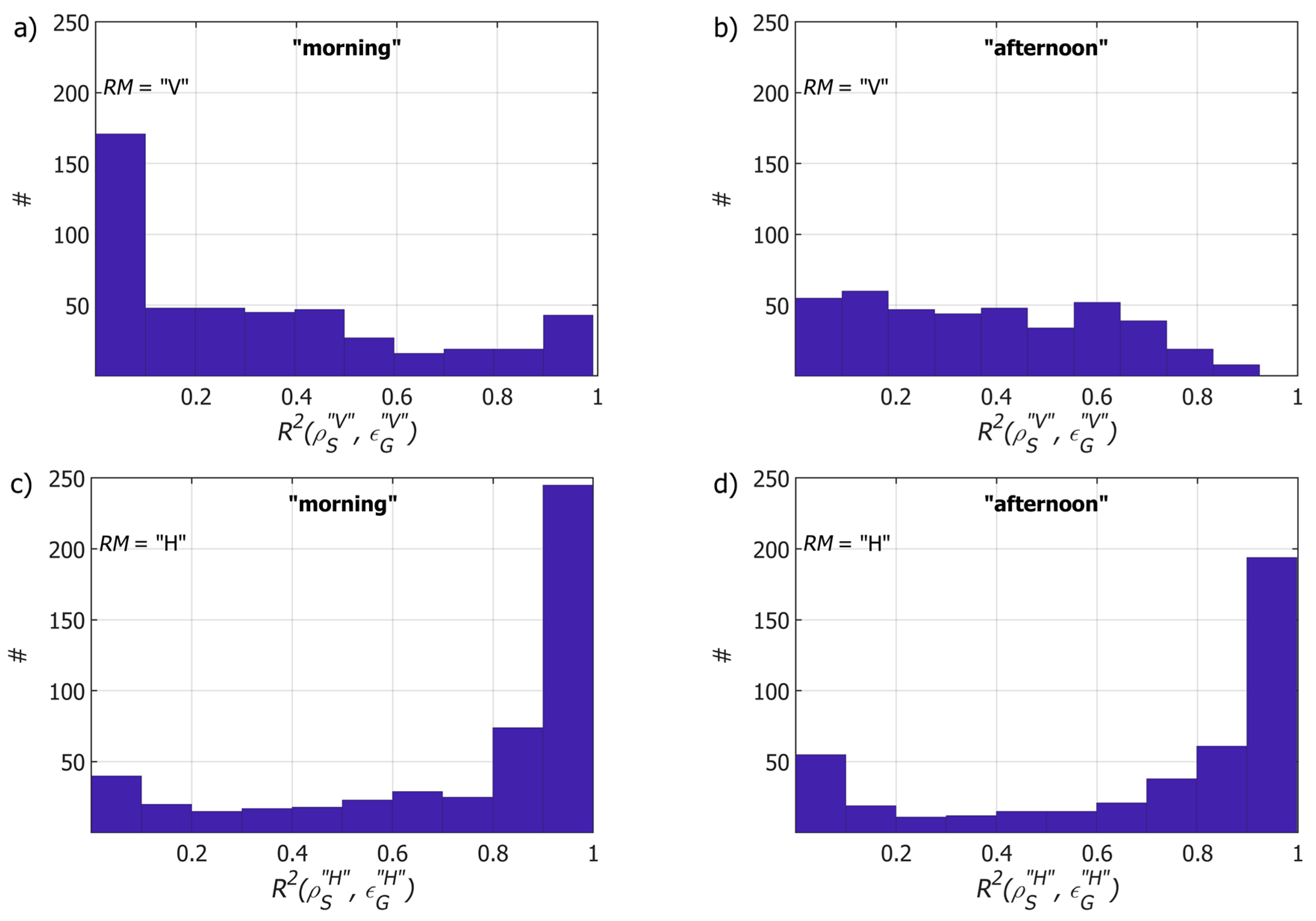
Figure 8.
Multi-angle two-parameter retrievals for the time period 15 December, 2016–15 March, 2017. Panels (a,b) show the time series of and , respectively. Panels (c,d) and (e,f) show corresponding and for RM = “H” and “V”, respectively. Red markers show in-situ measured bottom-layer snow density and ground permittivity (same data as shown in Figure 2). The vertical dashed lines delimit the “snow-free period” (before 3 January), the “cold winter period” (3–31 January), and the “early spring period” (after 31 January). Retrievals are in red when the “quality flag” is raised and in blue when not raised. The “quality flag” approach used employs the threshold between retrievals computed from 12-hour asymmetric sliding windows.

Figure 9.
(a,b) Time series of the footprint-specific and single-angle retrievals from 3 January (first snow event) to 15 March (end of measurement campaign). Colored bars show the color code of the retrievals performed at nadir angles labelled on the left vertical axes. Failed retrievals are shown in blue.

Figure 10.
(a) Single-angle retrievals for (blue) and for (red). (b) Comparison of single-angle retrievals for (blue) with multi-angle retrievals (red, same as in Figure 6a). Spatially averaged in-situ references (same as in Figure 2a,b) and their spatial variability are shown by the green lines and gray areas, respectively. The specific date 21 February is marked with the vertical dashed black line.

© 2018 by the authors. Licensee MDPI, Basel, Switzerland. This article is an open access article distributed under the terms and conditions of the Creative Commons Attribution (CC BY) license (http://creativecommons.org/licenses/by/4.0/).
Share and Cite
MDPI and ACS Style
Schwank, M.; Naderpour, R. Snow Density and Ground Permittivity Retrieved from L-Band Radiometry: Melting Effects. Remote Sens. 2018, 10, 354. https://doi.org/10.3390/rs10020354
AMA Style
Schwank M, Naderpour R. Snow Density and Ground Permittivity Retrieved from L-Band Radiometry: Melting Effects. Remote Sensing. 2018; 10(2):354. https://doi.org/10.3390/rs10020354
Chicago/Turabian StyleSchwank, Mike, and Reza Naderpour. 2018. "Snow Density and Ground Permittivity Retrieved from L-Band Radiometry: Melting Effects" Remote Sensing 10, no. 2: 354. https://doi.org/10.3390/rs10020354
Note that from the first issue of 2016, this journal uses article numbers instead of page numbers. See further details here.