Joint Sparse and Low-Rank Multitask Learning with Laplacian-Like Regularization for Hyperspectral Classification

Abstract

Multitask learning (MTL) has recently provided significant performance improvements in supervised classification of hyperspectral images (HSIs) by incorporating shared information across multiple tasks. However, the original MTL cannot effectively exploit both local and global structures of the HSI and the class label information is not fully used. Moreover, although the mathematical morphology (MM) has attracted considerable interest in feature extraction of HSI, it remains a challenging issue to sufficiently utilize multiple morphological profiles obtained by various structuring elements (SEs). In this paper, we propose a joint sparse and low-rank MTL method with Laplacian-like regularization (termed as sllMTL) for hyperspectral classification by utilizing the three-dimensional morphological profiles (3D-MPs) features. The main steps of the proposed method are twofold. First, the 3D-MPs are extracted by the 3D-opening and 3D-closing operators. Different SEs are adopted to result in multiple 3D-MPs. Second, sllMTL is proposed for hyperspectral classification by taking the 3D-MPs as features of different tasks. In the sllMTL, joint sparse and low-rank structures are exploited to capture the task specificity and relatedness, respectively. Laplacian-like regularization is also added to make full use of the label information of training samples. Experiments on three datasets demonstrate the OA of the proposed method is at least about 2% higher than other state-of-the-art methods with very limited training samples.

1. Introduction

By simultaneously acquiring hundreds of continuous narrow spectral wavelengths for each image pixel, hyperspectral remote sensors can generate three-dimensional (3D) hyperspectral cubes containing rich spectral and spatial information. Thanks to the high spectral and spatial resolution, hyperspectral images (HSIs) have opened up new avenues for the remote sensing applications, including earth observation [1], environmental science [2], agriculture [3], mineral identification [4], etc. Supervised classification [5,6,7,8], which aims at assigning each pixel in the HSI into an accurate class label with representative training samples, plays an important role in those applications. However, it still faces some challenges in the classification task. For example, a large number of labeled samples are crucial to producing good classification results due to the Hughes phenomenon, but in reality, it is extremely difficult even impossible to identify the labels of samples. Other difficulties, such as the spectral signature from identical material may vary while different materials may have similar signatures, will also give a negative effect on the classification performance.

Much work has been carried out in the literature to address the above-mentioned dilemmas. The first category is to design reliable classifiers, among which support vector machine (SVM) [9,10] is one of the state-of-the-art methods. The success of SVM stems from the fact that it is robust to the high spectral dimension by using kernel tricks. Variations of the SVM-based methods are proposed to improve the classification performance, such as incorporating spatial information by composite kernels (SVMCK) [11] or multiple kernels [12], combining the kernel matrices of a family of SVM classifiers by ensemble learning [13], and the semi-supervised learning extension [14,15] by exploiting both labeled and unlabeled samples, etc. However, the kernel tricks in the SVM require proper tuning of parameters. Sparse representation-based classification (SRC), which is pioneered by Wright et al. [16] for face recognition, has become another widely used hyperspectral classifier [17,18,19,20,21,22,23,24,25]. The SRC is suitable for classifying the HSIs because it relies on the assumption that the spectral signatures of hyperspectral pixels belonging to the same class approximately lie in the same low-dimensional subspace and the unknown test sample can be sparsely represented by a linear combination of a few atoms from the whole training dictionary. Haq et al. [26] propose a homotopy-based SRC to alleviate the problem introduced by the high-dimensional data with too few labeled samples. The contextual information of neighboring pixels can also be incorporated to solve the problem of lack of sufficient training samples [18,19,22,23]. Multitask learning (MTL) [27,28,29,30,31], which can learn shared information across multiple tasks, has also demonstrated to be very powerful. In [28], several complementary features (i.e., spectral, gradient, Gabor texture and shape) are combined in a MTL fusion to enhance the discrimination of hyperspectral pixels, while kernel joint collaborative representation with adaptive weighted MTL is proposed in [29] to obtain desirable classification results. A SVM-based MTL method is proposed in [31] to effectively utilize the rich information included in the extracted two-dimensional (2D) Gabor features. Although many contributions have been carried out to improve the classification performance of MTL, till now, existing MTL methods rarely exploit both the task specificity and relatedness, and the label information of the training samples is also not fully utilized.

The second category is to increase the class separability by feature extraction/selection. Apart from spectral profiles, the spatial context can be adopted to improve the classification results. Many spatial filters have been proposed over the past few years, such as the edge-preserving filtering [5,32] and the mathematical morphology (MM) processing [33,34], where the spatial-domain features are extracted by edge-preserving filter or opening/closing operators. In [32], the edge-preserving filtering is conducted on the probability maps (i.e., probability presentation of the classification maps) and the label of a test sample is determined by maximum probability. In [5], a principal component analysis (PCA)-based edge-preserving method is proposed to highlight the separability of pixels. This simple yet powerful filtering approach has announced impressive results for hyperspectral classification. The MM-based method proposed in [33,34] is termed as extended morphological profile (EMP), where the opening and closing operators with different sizes of structuring elements (SEs) are performed on the first several principal components. It is worth stressing that a HSI data is naturally formed as a 3D cube consisting of a spectral dimension and two spatial dimensions. However, the above-mentioned methods ignore the 3D nature of the HSI.

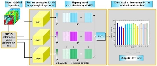
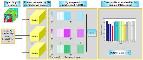
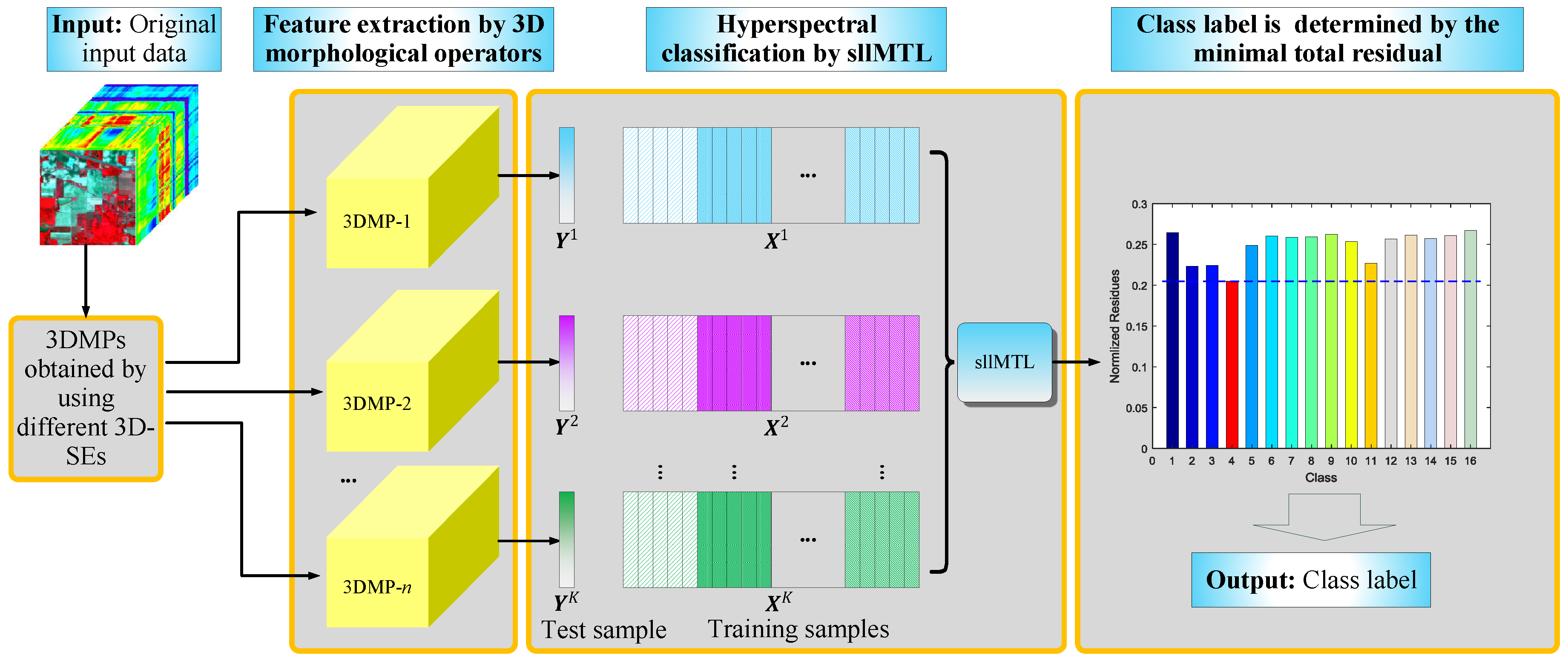
In this paper, we propose a joint sparse and low-rank MTL method with Laplacian-like regularization (abbreviated as sllMTL) for classification of HSI by utilizing the 3D morphological profiles (3D-MPs). The visual illustration of the proposed method is shown in Figure 1, which is consisted of two major steps. In the feature extraction step, the 3D-MPs [35] of the HSI are obtained by the 3D-opening and 3D-closing operators with various SEs. Each SE can produce two corresponding 3D-MPs (one is obtained by the 3D-opening and another is generated by the 3D-closing). The significant difference between the existing 3D-MPs-based method [35] and our proposed method is that: other than simply stacking multiple 3D-MPs together, we make full use of the 3D-MPs cubes simultaneously in a MTL manner. In the classification step, the sllMTL is proposed to exploit the joint sparse and low-rank structures by treating each 3D-MP as the feature of a specific task. Both sparse and low-rank constraints are added to the representation coefficients so as to capture the task specificity and relatedness. A Laplacian-like regularization is also adopted to take advantage of the class label information. Finally, the class label of the test sample can be determined by the minimal total residual.

The advantages of the proposed method lie in the following two aspects:

• 3D-MPs are adopted for feature extraction of the HSI cube. Compared to the vector/image-based methods, we respect the 3D nature of the HSI and take the HSI cube as a whole entity to simultaneously extract the spectral-spatial features. Different from the existing 3D-MPs-based method, we do not simply stack multiple 3D-MPs but fully exploit the spectral-spatial feature of each 3DMP in a novel MTL framework.
• sllMTL is proposed to simultaneously classify the 3D-MPs by taking each 3D-MP as the feature of a specific task. Compared to the existing MTL, the proposed sllMTL can capture both specificities and shared factors of the tasks by utilizing the sparse and low-rank constraints. Moreover, the Laplacian-like regularization can improve the classification performance further by making full use of the class label information.

The remainder of this paper is organized as follows. Section 2 introduces two types of 3D mathematical morphology methods (i.e., 3D-opening and 3D-closing operators) to obtain multiple 3D-MPs. Section 3 describes the proposed sllMTL for hyperspectral classification in detail. Section 4 shows the experimental results, and discussions and conclusions are drawn in Section 5 and Section 6.

2. Multiple Morphological Profiles Extracted by 3D Mathematical Morphology

Although the EMP has been successfully employed in feature extraction of the HSI, it ignores the 3D nature of the hyperspectral cube and thus cannot fully investigate the 3D spectral-spatial dependence among pixels. In this section, 3D mathematical operators (i.e., 3D-opening and 3D-closing) are applied for multiple morphological profiles extraction of HSI.

MM is initially proposed as a rigorous theoretic framework for analyzing the spatial relationship of different pixels by using SEs with given shapes and sizes as input. The relationship and structural character of the image can be captured by keeping the SEs sliding over the image. In analogy to the 2D MM operators, the 3D extension ones learn the structural characters through the moving of 3D-SEs in the image. The major advantage of the 3D-SEs lies in that they can effectively explore the spectral-spatial structure of the 3D images (e.g., HSI). It is noteworthy that erosion and dilation are two basic morphological operators. Suppose the original HSI cube is represented as $\mathit{I}\in {\mathbb{R}}^{m\times n\times b}$, where $m,n$ and b refer to the number of rows, columns and spectral bands, respectively, the value in the cube $\mathit{I}$ for a given coordinate $(x_0,y_0,z_0)$ is $\mathit{I}(x_0,y_0,z_0)$ with $\mathit{I}(x_0,y_0,z_0)\in \mathbb{R}$, $\mathit{B}$ is a 3D-SE and $\mathit{B}(x_0,y_0,z_0)$ indicates a set of values centered at the coordinate $(x_0,y_0,z_0)$ of $\mathit{I}$, the 3D-erosion ${ϵ}_{\mathit{B}}^{3D}(\mathit{I}(x_0,y_0,z_0))$ of the cube $\mathit{I}$ at the coordinate $(x_0,y_0,z_0)$ with the 3D-SE $\mathit{B}$ is determined by the minimum value of pixels inside $\mathit{B}(x_0,y_0,z_0)$

$${ϵ}_{\mathit{B}}^{3D}(\mathit{I}(x_0,y_0,z_0))=\mathit{I}\ominus \mathit{B}=\underset{(x,y,z)}{min}(\mathit{I}(x,y,z)\in \mathit{B}(x_0,y_0,z_0))$$

(1)

where “⊖” indicates the 3D-erosion operator.

The 3D-dilation ${\delta }_{\mathit{B}}^{3D}(\mathit{I}(x_0,y_0,z_0))$ can be regarded as the dual operator, which switches the minimum operator to the maximum one

$${\delta }_{\mathit{B}}^{3D}(\mathit{I}(x_0,y_0,z_0))=\mathit{I}\oplus \mathit{B}=\underset{(x,y,z)}{max}(\mathit{I}(x,y,z)\in \mathit{B}(x_0,y_0,z_0))$$

(2)

where “⊕” indicates the 3D-dilation operator.

The 3D-erosion can expand objects of the HSI cube that are darker than their neighborhoods, while the 3D-dilation shrinks them, and vice versa for the objects that are brighter than their neighborhoods. The 3D-opening and 3D-closing operators can be derived from the combination of 3D-erosion and 3D-dilation. In greater detail, the 3D-opening ${\gamma }_{\mathit{B}}^{3D}(\mathit{I})$ is calculated by the 3D-erosion of the HSI cube $\mathit{I}$ with $\mathit{B}$ followed by the 3D-dilation with $\mathit{B}$

$${\gamma }_{\mathit{B}}^{3D}(\mathit{I})=\mathit{I}\circ \mathit{B}=(\mathit{I}\ominus \mathit{B})\oplus \mathit{B}={\delta }_{\mathit{B}}^{3D}({ϵ}_{\mathit{B}}^{3D}(\mathit{I}))$$

(3)

where “∘” indicates the 3D-opening operator.

Similarly, the 3D-closing ${\varphi }_{\mathit{B}}^{3D}(\mathit{I})$ can be obtained by the 3D-dilation of the HSI cube $\mathit{I}$ with $\mathit{B}$ followed by the 3D-erosion with $\mathit{B}$

$${\varphi }_{\mathit{B}}^{3D}(\mathit{I})=\mathit{I}•\mathit{B}=(\mathit{I}\oplus \mathit{B})\ominus \mathit{B}={ϵ}_{\mathit{B}}^{3D}({\delta }_{\mathit{B}}^{3D}(\mathit{I}))$$

(4)

where “•” indicates the 3D-closing operator.

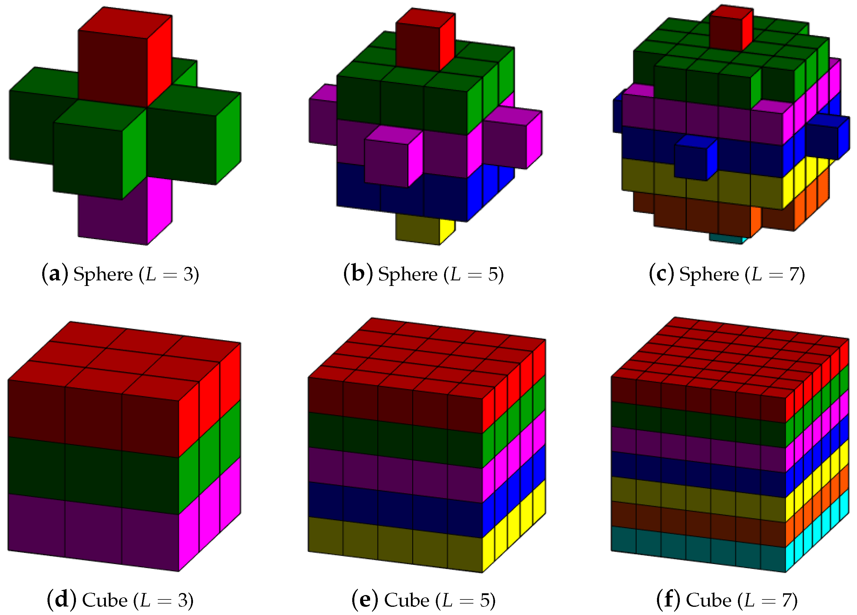
The multiple 3D-MPs of $\mathit{I}$ in our proposed method are generated by performing a series of 3D-opening and 3D-closing operators with different 3D-SEs. As an example, Figure 2 depicts a set of 3D-SEs with various shapes (e.g., cube, sphere) and sizes (e.g., side length (L) is set to 3, 5 and 7). Each 3D-SE can produce two corresponding 3D-MPs in merit of the 3D-opening and 3D-closing, respectively.

3. Joint Sparse and Low-Rank Multitask Learning with Laplacian-Like Regularization

In this section, we propose the sllMTL method to exploit both the local and global structures of the HSI by taking the 3D-MPs obtained from the 3D-opening and 3D-closing morphological operators as features of multiple tasks. Both sparse and low-rank constraints are considered in the sllMTL to capture the task specificity and relatedness. Moreover, Laplacian-like regularization is also added to improve the classification performance by taking full advantage of the label information of training samples. Suppose K 3D-MPs are generated by the 3D morphological operators, there are K tasks in the sllMTL. For each task index $k=1,2,\dots ,K$, represent ${\mathit{X}}^k=[{\mathit{X}}_1^k,{\mathit{X}}_2^k,\dots ,{\mathit{X}}_J^k]$ as the training feature matrix, in which ${\mathit{X}}_j^k\in {\mathbb{R}}^{m_k\times p_j},j=1,2,\dots ,J$ is related to the jth class, J indicates the total number of classes contained in the HSI, $m_k$ refers to the dimensionality of the kth task (note that no feature reduction is performed, $m_k$ equals to the number of spectral bands b), $p_j$ denotes the number of training samples belong to class j, and ${\sum }_{j=1}^J{p}_j=P$ is the total number of training samples. Given the unlabeled test sample $\mathit{Y}=[{\mathit{Y}}^1,{\mathit{Y}}^2,\dots ,{\mathit{Y}}^K]$, the sllMTL method is formulated as the solution to the following problem

$$\begin{array}{cc}\underset{\mathit{Z}}{min}& {\parallel \mathit{Z}\parallel }_{\ast }+\lambda {\parallel \mathit{Z}\parallel }_{1,2}+\beta \mathrm{tr}({\mathit{Z}}^{\mathrm{T}}\mathit{L}\mathit{Z})\hfill \\ s.t.& {\mathit{Y}}^k={\mathit{X}}^k{\mathit{Z}}^k,k=1,2,\dots ,K\hfill \end{array}$$

(5)

where $\mathit{Z}$ denotes the coefficient matrix to be calculated, joint sparse and low-rank constraints are added to $\mathit{Z}$, ${\parallel \mathit{Z}\parallel }_{\ast }$ refers to the trace norm (also known as the nuclear norm, i.e., the sum of singular values of a matrix), which can be utilized to identify the shared characters among multiple tasks, ${\parallel \mathit{Z}\parallel }_{1,2}$ indicates the row-sparse constraint to identify the task specificities, $\mathit{L}$ is the Laplacian-like matrix, $\mathrm{tr}(·)$ is the trace of a matrix, i.e., the sum of the elements on the main diagonal. The matrix $\mathit{L}$ is generated by the natural assumption that the coefficients ${\mathit{Z}}_p$ and ${\mathit{Z}}_{\tilde{p}}$, $p,\tilde{p}=1,2,\dots ,P$ from the same class are more closer or similar than those belong to different classes. This assumption can be realized in terms of similarity. In mathematics, a reasonable way is to minimize the following function

$$\begin{array}{ccc}\frac{1}{2}{\displaystyle \sum _{p,\tilde{p}=1}^P}{\parallel {\mathit{Z}}_p-{\mathit{Z}}_{\tilde{p}}\parallel }_2^2{\mathit{W}}_{p\tilde{p}}\hfill & =\hfill & {\displaystyle \sum _{p=1}^P}{\mathit{Z}}_p{\mathit{Z}}_p^{\mathrm{T}}{\mathit{D}}_{pp}-{\displaystyle \sum _{p,\tilde{p}=1}^P}{\mathit{Z}}_p{\mathit{Z}}_{\tilde{p}}^{\mathrm{T}}{\mathit{W}}_{p\tilde{p}}\hfill \\ & =\hfill & \mathrm{tr}({\mathit{Z}}^{\mathrm{T}}\mathbf{DZ})-\mathrm{tr}({\mathit{Z}}^{\mathrm{T}}\mathit{WZ})\hfill \\ & =\hfill & \mathrm{tr}({\mathit{Z}}^{\mathrm{T}}\mathit{LZ})\hfill \end{array}$$

(6)

where $\mathit{D}$ is a diagonal matrix in which ${\mathit{D}}_{pp}={\sum }_{\tilde{p}=1}^P{\mathit{W}}_{p\tilde{p}}$, $\mathit{L}$ is the Laplacian-like matrix obtained by $\mathit{L}=\mathit{D}-\mathit{W}$, and ${\mathit{W}}_{p\tilde{p}}=\left\{\begin{array}{cc}1& \mathrm{if}\mathrm{the}p\mathrm{th}\mathrm{and}\tilde{p}\mathrm{th}\mathrm{training}\mathrm{samples}\mathrm{belong}\mathrm{to}\mathrm{the}\mathrm{same}\mathrm{class}\hfill \\ 0& \mathrm{otherwise}\hfill \end{array}\right.$. To give an intuitive explanation, Figure 3 visually shows the $\mathit{W}$ used in the three HSI datasets. It should be mentioned that the label information of the training samples are adopted to obtain the matrix $\mathit{W}$, which can then be utilized to generate $\mathit{L}$ ($\mathit{L}=\mathit{D}-\mathit{W}$) in Equation (5). Therefore, the training samples are utilized more fully in the proposed method. Moreover, although we add a Laplacian-like regularization in the joint sparse and low-rank multitask learning method, it cannot state that the Laplacian-like regularization is more effective than the sparse and low-rank regularizations. Actually, the Laplacian-like regularization is complementary to the sparse and low-rank regularizations. Note that the usage of the low-rank and sparsity priors have achieved great success in HSI classification, we also use the joint sparse and low-rank regularizations (i.e., ${\parallel \mathit{Z}\parallel }_{\ast }$ and ${\parallel \mathit{Z}\parallel }_{1,2}$) in the proposed method (see Equation (5)).

To solve Equation (5), we first introduce two auxiliary matrices $\mathit{P}$ and $\mathit{Q}$ to make the optimization problem in Equation (5) separable and simplify the solution procedure, in this regard, the problem in Equation (5) can be rewritten as

$$\begin{array}{cc}\underset{\mathit{Z},\mathit{P},\mathit{Q}}{min}& {\parallel \mathit{P}\parallel }_{\ast }+\lambda {\parallel \mathit{Q}\parallel }_{1,2}+\beta \mathrm{tr}({\mathit{P}}^{\mathrm{T}}\mathit{L}\mathit{P})\hfill \\ s.t.& {\mathit{Y}}^k={\mathit{X}}^k{\mathit{Z}}^k,{\mathit{Z}}^k={\mathit{Q}}^k,{\mathit{Z}}^k={\mathit{P}}^k,k=1,2,\dots ,K\hfill \end{array}$$

(7)

Linearized alternating direction method with Adaptive Penalty (LADMAP) [36] can be adopted to solve the above-mentioned problem, whose augmented Lagrangian function yields

$$\begin{array}{ccc}\mathcal{L}(\mathit{Z},\mathit{P},\mathit{Q})& =\hfill & {\parallel \mathit{P}\parallel }_{\ast }+\lambda {\parallel \mathit{Q}\parallel }_{1,2}+\beta \mathrm{tr}({\mathit{P}}^{\mathrm{T}}\mathit{L}\mathit{P})\hfill \\ & +\hfill & {\displaystyle \sum _{k=1}^K}\{<{\mathit{M}}_1^k,{\mathit{Y}}^k-{\mathit{X}}^k{\mathit{Z}}^k>+<{\mathit{M}}_2^k,{\mathit{Z}}^k-{\mathit{Q}}^k>+<{\mathit{M}}_3^k,{\mathit{Z}}^k-{\mathit{P}}^k>\hfill \\ & +\hfill & \frac{\mu }{2}\left(\parallel {\mathit{Y}}^k-{\mathit{X}}^k{\mathit{Z}}^k{\parallel }_{\mathrm{F}}^2+\parallel {\mathit{Z}}^k-{\mathit{Q}}^k{\parallel }_{\mathrm{F}}^2+{\parallel {\mathit{Z}}^k-{\mathit{P}}^k\parallel }_{\mathrm{F}}^2\right)\}\hfill \end{array}$$

(8)

where $\mu >0$ is a penalty parameter, ${\mathit{M}}_1^k,{\mathit{M}}_2^k,k=1,2,\cdots ,K$ are Lagrange multipliers, ${\mathit{Z}}^k,{\mathit{P}}^k,{\mathit{Q}}^k$ are the kth column of $\mathit{Z},\mathit{P},\mathit{Q}$, respectively, and ${\parallel ·\parallel }_{\mathrm{F}}$ is the Frobenius norm obtained by the square root of the sum of the absolute squares of matrix elements, e.g., ${\parallel \mathit{A}\parallel }_{\mathrm{F}}=\sqrt{{\sum }_i{\sum }_j{\left|a_{ij}\right|}^2}$.

The variables $\mathit{Z},\mathit{P}$ and $\mathit{Q}$ can be updated alternately by minimizing the augmented Lagrangian function (see Equation (8)) with other variables fixed. In case the augmented Lagrangian function is difficult to minimize with a specific variable, we will linearize the corresponding smooth component. Specifically, the updating process is as follows.

Fix other variables, and the variable $\mathit{P}$ in the $(t+1)$th iteration can be updated by minimizing $\mathcal{L}({\mathit{Z}}^{(t)},\mathit{P},{\mathit{Q}}^{(t)})$

$$\begin{array}{ccc}{\mathit{P}}^{(t+1)}& =\hfill & \arg \underset{\mathit{P}}{min}\mathcal{L}({\mathit{Z}}^{(t)},\mathit{P},{\mathit{Q}}^{(t)})\hfill \\ & =\hfill & \arg \underset{\mathit{P}}{min}{\parallel \mathit{P}\parallel }_{\ast }+\beta \mathrm{tr}({\mathit{P}}^{\mathrm{T}}\mathit{L}\mathit{P})+\frac{\mu }{2}{\displaystyle \sum _{k=1}^K}\left\{\frac{2}{\mu }<{\mathit{M}}_3^{k,(t)},{\mathit{Z}}^{k,(t)}-{\mathit{P}}^k>+{\parallel {\mathit{Z}}^{k,(t)}-{\mathit{P}}^k\parallel }_{\mathrm{F}}^2\right\}\hfill \\ & =\hfill & \arg \underset{\mathit{P}}{min}{\parallel \mathit{P}\parallel }_{\ast }+\beta \mathrm{tr}({\mathit{P}}^{\mathrm{T}}\mathit{L}\mathit{P})+\frac{\mu }{2}{\displaystyle \sum _{k=1}^K}\left\{\parallel {\mathit{Z}}^{k,(t)}-{\mathit{P}}^k+\frac{{\mathit{M}}_3^{k,(t)}}{\mu }{\parallel }_{\mathrm{F}}^2\right\}\hfill \\ & =\hfill & \arg \underset{\mathit{P}}{min}{\parallel \mathit{P}\parallel }_{\ast }+\beta \mathrm{tr}({\mathit{P}}^{\mathrm{T}}\mathit{L}\mathit{P})+\frac{\mu }{2}\parallel {\mathit{Z}}^{(t)}-\mathit{P}+\frac{{\mathit{M}}_3^{(t)}}{\mu }{\parallel }_{\mathrm{F}}^2\hfill \\ & =\hfill & \arg \underset{\mathit{P}}{min}{\parallel {\mathit{P}}^{\mathrm{T}}\parallel }_{\ast }+\beta \mathrm{tr}({\mathit{P}}^{\mathrm{T}}\mathit{L}\mathit{P})+\frac{\mu }{2}\parallel {\left({\mathit{Z}}^{(t)}-\mathit{P}+\frac{{\mathit{M}}_3^{(t)}}{\mu }\right)}^{\mathrm{T}}{\parallel }_{\mathrm{F}}^2\hfill \\ & =\hfill & \arg \underset{\tilde{\mathit{P}}}{min}{\parallel \tilde{\mathit{P}}\parallel }_{\ast }+\beta \mathrm{tr}(\tilde{\mathit{P}}\mathit{L}{\tilde{\mathit{P}}}^{\mathrm{T}})+\frac{\mu }{2}\parallel {\mathit{Z}}^{(t)\mathrm{T}}-\tilde{\mathit{P}}+\frac{{\mathit{M}}_3^{(t)\mathrm{T}}}{\mu }{\parallel }_{\mathrm{F}}^2\hfill \end{array}$$

(9)

where $\tilde{\mathit{P}}={\mathit{P}}^{\mathrm{T}}$.

Note that Equation (9) does not have a closed-form solution, we express the smooth component of $\mathcal{L}({\mathit{Z}}^{(t)},\mathit{P},{\mathit{Q}}^{(t)})$ as

$$\begin{array}{ccc}\hfill q(\tilde{\mathit{P}})& =& \beta \mathrm{tr}(\tilde{\mathit{P}}\mathit{L}{\tilde{\mathit{P}}}^{\mathrm{T}})+\frac{\mu }{2}\parallel {\mathit{Z}}^{(t)\mathrm{T}}-\tilde{\mathit{P}}+\frac{{\mathit{M}}_3^{(t)\mathrm{T}}}{\mu }{\parallel }_{\mathrm{F}}^2\hfill \end{array}$$

(10)

Inspired by the LADMAP method, minimizing $\mathcal{L}({\mathit{Z}}^{(t)},\mathit{P},{\mathit{Q}}^{(t)})$ can be approximately substituted by solving the following problem

$$\begin{array}{ccc}{\tilde{\mathit{P}}}^{(t+1)}& \approx \hfill & \arg \underset{\mathit{P}={\tilde{\mathit{P}}}^{\mathrm{T}}}{min}\parallel \tilde{\mathit{P}}{\parallel }_{\ast }+<{\nabla }_{\tilde{\mathit{P}}}q({\tilde{\mathit{P}}}^{(t)}),\tilde{\mathit{P}}-{\tilde{\mathit{P}}}^{(t)}>+\frac{\eta }{2}\parallel \tilde{\mathit{P}}-{\tilde{\mathit{P}}}^{(t)}{\parallel }_{\mathrm{F}}^2\hfill \\ & =\hfill & \arg \underset{\mathit{P}={\tilde{\mathit{P}}}^{\mathrm{T}}}{min}\frac{1}{\eta }\parallel \tilde{\mathit{P}}{\parallel }_{\ast }+\frac{1}{\eta }<{\nabla }_{\tilde{\mathit{P}}}q({\tilde{\mathit{P}}}^{(t)}),\tilde{\mathit{P}}-{\tilde{\mathit{P}}}^{(t)}>+\frac{1}{2}\parallel \tilde{\mathit{P}}-{\tilde{\mathit{P}}}^{(t)}{\parallel }_{\mathrm{F}}^2\hfill \\ & =\hfill & \arg \underset{\mathit{P}={\tilde{\mathit{P}}}^{\mathrm{T}}}{min}\frac{1}{\eta }{\parallel \tilde{\mathit{P}}\parallel }_{\ast }+\frac{1}{2}\left\{\frac{2}{\eta }<{\nabla }_{\tilde{\mathit{P}}}q({\tilde{\mathit{P}}}^{(t)}),\tilde{\mathit{P}}-{\tilde{\mathit{P}}}^{(t)}>+\parallel \tilde{\mathit{P}}-{\tilde{\mathit{P}}}^{(t)}{\parallel }_{\mathrm{F}}^2\right\}\hfill \\ & =\hfill & \arg \underset{\mathit{P}={\tilde{\mathit{P}}}^{\mathrm{T}}}{min}\frac{1}{\eta }{\parallel \tilde{\mathit{P}}\parallel }_{\ast }+\frac{1}{2}\left(\parallel \tilde{\mathit{P}}-{\tilde{\mathit{P}}}^{(t)}+\frac{1}{\eta }{\nabla }_{\tilde{\mathit{P}}}q({\tilde{\mathit{P}}}^{(t)}){\parallel }_{\mathrm{F}}^2\right)\hfill \end{array}$$

(11)

where $q(\tilde{\mathit{P}})$ is approximated by its linearization $<{\nabla }_{\tilde{\mathit{P}}}q({\tilde{\mathit{P}}}^{(t)}),\tilde{\mathit{P}}-{\tilde{\mathit{P}}}^{(t)}>$ at ${\tilde{\mathit{P}}}^{(t)}$ plus a proximal term $\frac{\eta }{2}{\parallel \tilde{\mathit{P}}-{\tilde{\mathit{P}}}^{(t)}\parallel }_{\mathrm{F}}^2$, and ${\nabla }_{\tilde{\mathit{P}}}q({\tilde{\mathit{P}}}^{(t)})$ denotes the gradient of q w.r.t. $\tilde{\mathit{P}}$. As long as ${\eta >2\beta \parallel \mathit{L}\parallel }_2+\mu$, the above substitution is valid. Therefore, the Equation (11) has a closed-form solution formulated as

$$\begin{array}{ccc}{\tilde{\mathit{P}}}^{(t+1)}& =\hfill & {\mathcal{D}}_{{\mu }^{-1}}\left({\tilde{\mathit{P}}}^{(t)}-\frac{1}{\eta }{\nabla }_{\tilde{\mathit{P}}}q({\tilde{\mathit{P}}}^{(t)})\right)\hfill \\ & =\hfill & \mathit{U}{\mathcal{D}}_{{\mu }^{-1}}(\Sigma ){\mathit{V}}^{\mathrm{T}}\hfill \\ & =\hfill & \mathit{U}\mathrm{diag}\left({\left\{{\left({\pi }_i-\frac{1}{\mu }\right)}_{+}\right\}}_{1\le i\le \tilde{r}}\right){\mathit{V}}^{\mathrm{T}}\hfill \end{array}$$

(12)

where $\mathit{U}$ and $\mathit{V}$ are the matrices with orthogonal columns, ${(·)}_{+}=max(·,0)$, $\tilde{r}$ and ${\pi }_i$ refer to the rank and singular values of $\left({\tilde{\mathit{P}}}^{(t)}-\frac{1}{\eta }{\nabla }_{\tilde{\mathit{P}}}q({\tilde{\mathit{P}}}^{(t)})\right)$, respectively, and ${\mathit{P}}^{(t+1)}={\tilde{\mathit{P}}}^{(t+1)\mathrm{T}}$.

Fix the others, and the variable $\mathit{Q}$ in the $(t+1)$th iteration can be updated by

$$\begin{array}{ccc}{\mathit{Q}}^{(t+1)}& =\hfill & \arg \underset{\mathit{Q}}{min}\mathcal{L}({\mathit{Z}}^{(t)},{\mathit{P}}^{(t+1)},\mathit{Q})\hfill \\ & =\hfill & \arg \underset{\mathit{Q}}{min}\frac{\lambda }{\mu }{\parallel \mathit{Q}\parallel }_{1,2}+\frac{1}{2}\parallel \mathit{Q}-\left({\mathit{Z}}^{(t)}+\frac{{\mathit{M}}_2^{(t)}}{\mu }\right){\parallel }_{\mathrm{F}}^2\hfill \end{array}$$

(13)

which has the closed-form solution represented by the row-shrinkage thresholding operator.

Finally, fix the others and the variable $\mathit{Z}$ in the $(t+1)$th iteration can be updated by

$$\begin{array}{ccc}{\mathit{Z}}^{(t+1)}& =\hfill & \arg \underset{\mathit{Z}}{min}\mathcal{L}(\mathit{Z},{\mathit{P}}^{(t+1)},{\mathit{Q}}^{(t+1)})\hfill \\ & =\hfill & \arg \underset{\mathit{Z}}{min}{\displaystyle \sum _{k=1}^K}\{{\mathit{Z}}^{k,(t+1)\mathrm{T}}\left({\mathit{X}}^{k,(t+1)\mathrm{T}}{\mathit{X}}^{k,(t+1)}+2\mathit{I}\right){\mathit{Z}}^{k,(t+1)}-2{\mathit{Z}}^{k,(t+1)\mathrm{T}}({\mathit{X}}^{k,(t+1)\mathrm{T}}{\mathit{Y}}^{k,(t+1)}\hfill \\ & -\hfill & \frac{{\mathit{X}}^{k,(t+1)\mathrm{T}}{\mathit{M}}_1^{k,(t)}}{\mu }+{\mathit{Q}}^{k,(t+1)}-\frac{{\mathit{M}}_2^{k,(t)}}{\mu }+{\mathit{P}}^{k,(t+1)}-\frac{{\mathit{M}}_3^{k,(t)}}{\mu })\}\hfill \end{array}$$

(14)

According to Equation (14), the kth column of ${\mathit{Z}}^{(t+1)}$ yields

$$\begin{array}{ccc}\hfill {\mathit{Z}}^{k,(t+1)}& =& {\left({\mathit{X}}^{k,(t+1)\mathrm{T}}{\mathit{X}}^{k,(t+1)}+2\mathit{I}\right)}^{-1}{\mathit{H}}^{k,(t+1)}\hfill \end{array}$$

(15)

where ${\mathit{H}}^{k,(t+1)}={\mathit{X}}^{k,(t+1)\mathrm{T}}{\mathit{Y}}^{k,(t+1)}-\frac{{\mathit{X}}^{k,(t+1)\mathrm{T}}{\mathit{M}}_1^{k,(t)}}{\mu }+{\mathit{Q}}^{k,(t+1)}-\frac{{\mathit{M}}_2^{k,(t)}}{\mu }+{\mathit{P}}^{k,(t+1)}-\frac{{\mathit{M}}_3^{k,(t)}}{\mu }$ and $\mathit{I}$ is an identity matrix.

The above-mentioned equations are the major steps for updating the variables $\mathit{Z},\mathit{P},\mathit{Q}$. The detailed procedure for solving the optimization problem (see Equation (5)) in the proposed sllMTL method is summarized in Algorithm 1, in which $\mu$ is adjusted using an adaptive updating strategy [36] for faster convergence. As long as the coefficient matrix $\mathit{Z}$ is obtained, the label of the unlabeled test sample $\mathit{Y}$ can be determined by the minimal total residual

$$\begin{array}{ccc}\hfill \mathrm{Class}\mathit{Y}& =& arg\underset{j}{min}{r}_j=arg\underset{j}{min}{\displaystyle \sum _k^K}\parallel {\mathit{Y}}^k-{\mathit{X}}_j^k{\mathit{Z}}_j^k{\parallel }_2^2\hfill \end{array}$$

(16)

where ${\mathit{X}}_j^k$ and ${\mathit{Z}}_j^k$ are associated with the jth ($j=1,2,\dots ,J$) class.

Algorithm 1: LADMAP for Solving the Optimization Problem (see Equation (5)) in the Proposed sllMTL Method

Require:  The test feature matrix $\mathit{Y}$, the training feature matrix ${\mathit{X}}^k,k=1,2,\dots ,K$, and the parameters $\lambda$ and $\beta$ Ensure:  The solution $\mathit{Z}$ and class label of the unlabeled test sample $\mathit{Y}$   1: Initialize: $\mathit{Z}=\mathit{P}=\mathit{Q}={\mathit{M}}_2={\mathit{M}}_3=0$, ${\mathit{M}}_1=0$, $\rho =1.1$, $\mu ={10}^{-6}$, ${\mu }_{max}={10}^6$ and $t=0$   2: while Convergence is not attained do   3:  Fix the others and update the variable $\mathit{P}$ by Equation (12)   4:  Fix the others and update the variable $\mathit{Q}$ by Equation (13)   5:  Fix the others and update the variable $\mathit{Z}$ by Equation (15)   6:  Update the Lagrange multipliers ${\mathit{M}}_1,{\mathit{M}}_2$ and ${\mathit{M}}_3$ by     ${\mathit{M}}_1^{k,(t+1)}={\mathit{M}}_1^{k,(t)}+\mu ({\mathit{Y}}^{k,(t+1)}-{\mathit{X}}^{k,(t+1)}{\mathit{Z}}^{k,(t+1)})$     ${\mathit{M}}_2^{k,(t+1)}={\mathit{M}}_2^{k,(t)}+\mu ({\mathit{Z}}^{k,(t+1)}-{\mathit{Q}}^{k,(t+1)})$     ${\mathit{M}}_3^{k,(t+1)}={\mathit{M}}_3^{k,(t)}+\mu ({\mathit{Z}}^{k,(t+1)}-{\mathit{P}}^{k,(t+1)})$   7:  Update the parameter $\mu$ by $\mu =min({\mu }_{max},\rho \mu )$   8:  Update t by $t=t+1$   9: end while    10: Determine the class label of $\mathit{Y}$ by Equation (16)

4. Experiments

4.1. Dataset Description

In the experiments, we verify the performance of the proposed hyperspectral classification method on three benchmark datasets, i.e., the Indian Pines data, the University of Pavia data and the Salinas data. All the three hyperspectral datasets used in the experiments have been preprocessed by distortion correction. Details of each dataset are given below.

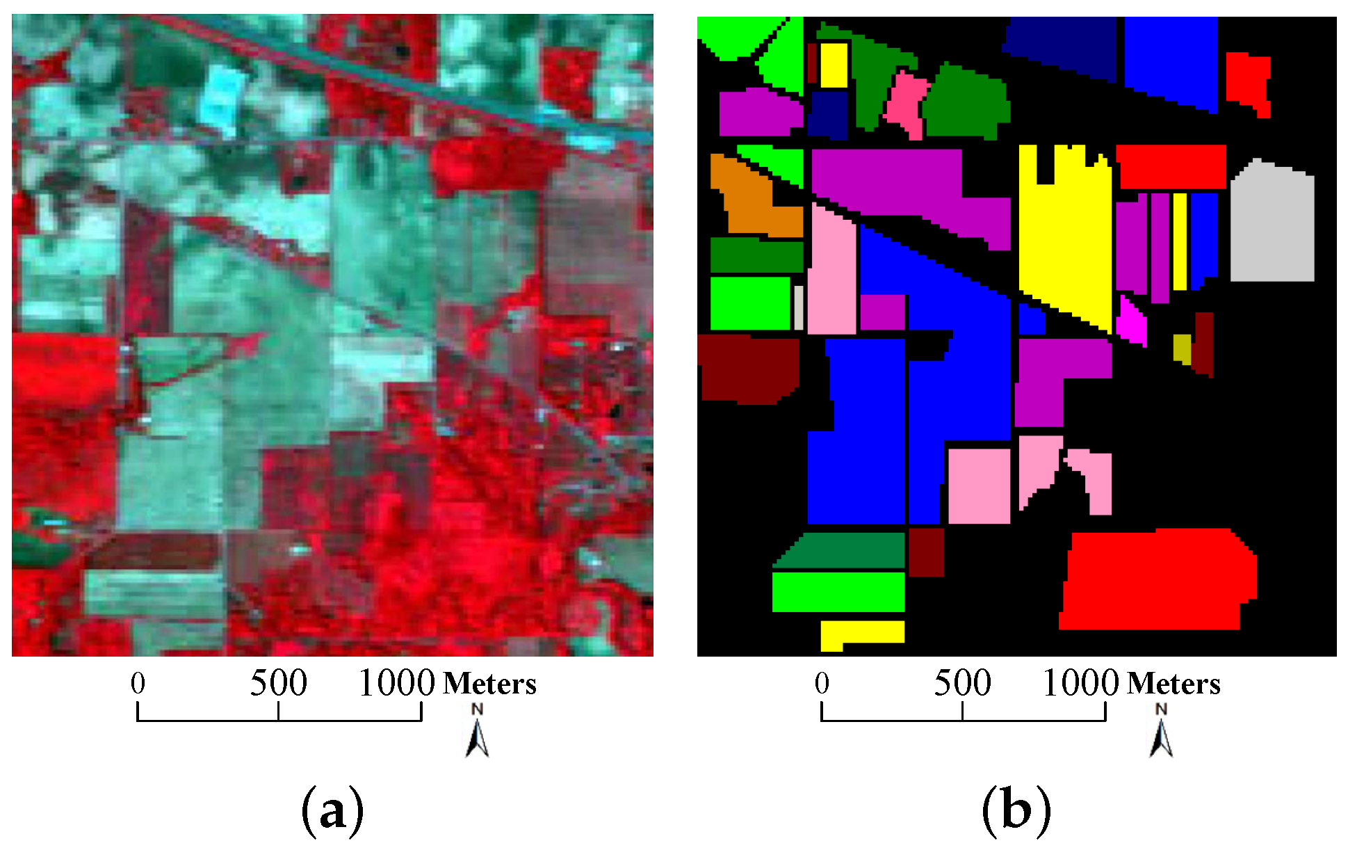
• Indian Pines data: the first data was gathered by the National Aeronautics and Space Administration’s (NASA) Airborne Visible/Infrared Imaging Spectrometer (AVIRIS) sensor on 12 June 1992 over the Indian Pines test site in Northwest Indiana, and it consists of $145\times 145$ pixels and 220 spectral reflectance bands cover the wavelength range of 0.4–2.5 $\mathsf{\mu }$m. The number of bands is reduced to 200 by removing the noisy and water-vapor absorption bands (bands 104–108, 150–163, and 220). The spatial resolution is about 20 m per pixel. Figure 4 depicts the three-band false color composite image together with its corresponding ground truth. The data contains 16 classes of interest land-covers and 10366 labeled pixels ranging unbalanced from 20 to 2468, which poses a big challenge to the classification problem.

  Table 1. Number of samples (NoS) used in the Indian Pines data.

  displays the detailed number of samples of each class, and the background color represents different classes of land-covers.
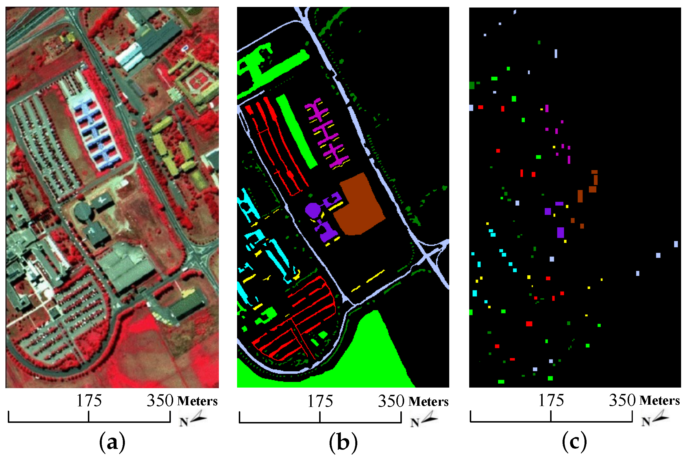
• University of Pavia data: the second dataset was captured by the Reflective Optics System Imaging Spectrometer (ROSIS) sensor on 8 July 2002 over an urban area surrounding the University of Pavia, Italy. It contains $610\times 340$ pixels with a spatial resolution of 1.3 m per pixel. The original dataset has 115 spectral channels with a coverage range from 0.43 to 0.86 $\mathsf{\mu }$m. 12 most noisy bands are removed before experiments, remaining 103 bands for experiments. 9 classes of interest are considered in this dataset. The color composite image, the ground truth data as well as the available training samples are depicted in Figure 5. As shown in

  Table 2. NoS and available training samples (NoATS) used in the University of Pavia data.

  , there are more than 900 pixels in each class, but the available training samples of each class are less than 600. In analogy to the Indian Pines data, the background color in Table 2 also agrees with that in Figure 5b,c.
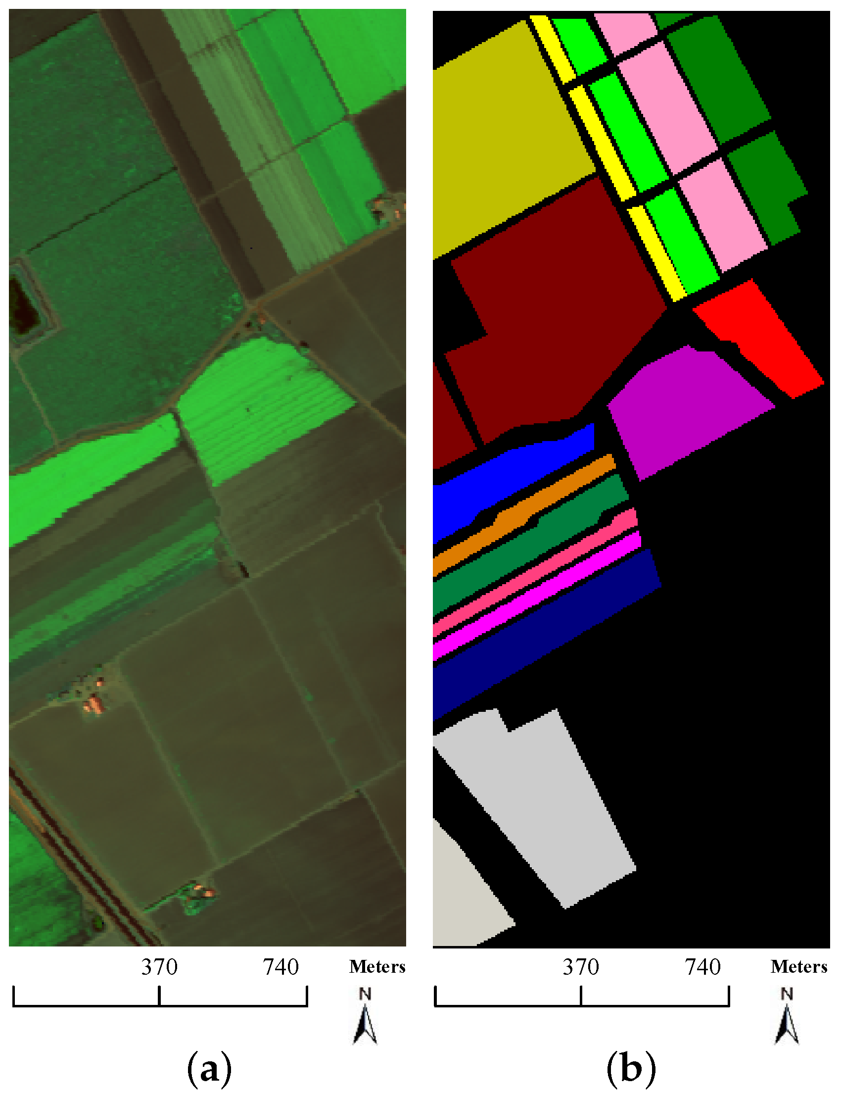
• Salinas data: the third dataset was acquired by the AVIRIS sensor on 8 October 1998 over the Salinas Valley, Southern California, USA. There are 224 bands in the original dataset, and 24 bands (bands 108–112, 154–167, and 224) are removed for the water absorption. The size of each band is $512\times 217$ pixels with a spatial resolution of 3.7 m per pixel. The color composite image and the ground truth are plotted in Figure 6. This dataset contains 16 classes of ground truth, and the detailed number of samples in each class is listed in

  Table 3. NoS used in the Salinas data.

  , whose background color corresponds to different classes of land-covers.

4.2. Experimental Design

To evaluate the effectiveness of the proposed method for hyperspectral classification, we compare our method with several baseline approaches, including the EMP [34], 3D discrete wavelet transform (3D-DWT) [37], SVM [9], SVMCK [11] and MTL [27]. The original spectral features (abbreviated as “Spec”) are also taken into consideration in the experiments. It is worthwhile to note that the “Spec”, EMP, 3D-DWT and 3D-MPs are feature extraction methods, whereas the SVM, SVMCK, MTL and sllMTL are classification methods. To investigate the performance of the proposed method in both feature extraction and classification, we compare the 3D-MPs with the “Spec”, EMP and 3D-DWT by fixing the classifier as sllMTL. Moreover, the sllMTL is compared with the SVM, SVMCK and MTL by utilizing the 3D-MPs-based features.

In greater detail, the 3D-MPs-based feature extraction method is validated by comparing with other widely-used methods, i.e., the original “Spec”, the multiple features obtained by the EMP, as well as the multiple features generated by the 3D-DWT. As to the above-mentioned feature extraction methods, (1) the original “Spec” features can be viewed as a special case of the sllMTL classifier with $K=1$. (2) The EMP does not use the PCA for dimensional reduction but obtains the morphological profiles by performing the opening/closing operators with various SEs on all of the bands. (3) The 3D-DWT-based multiple cubes consisted of the subcubes with different scales, frequencies and orientations are also used for comparison. (4) The 3D-MPs-based multiple cubes are obtained by directly performing the 3D-opening and 3D-closing on the HSI cubes using different 3D-SEs. The 3D-SEs adopted in 3D-MPs are the cube and sphere shapes. Note that there are large areas of homogeneous regions in the Indian Pines data and Salinas data, the side lengths of the 3D-SEs are set to $L=5,9,13,17$ and 21. Since many narrow regions are present in the University of Pavia data, smaller side lengths of 3D-SEs are chosen, i.e., $L=3,5,9,13$ and 17.

On the other hand, we test the performance of the sllMTL by fixing the input features as 3D-MPs and comparing the sllMTL with the SVM, SVMCK and MTL. Note that no nonlinear kernel is used in the proposed sllMTL, we adopt linear kernel in the SVM, SVMCK and MTL for consistency. For the SVM, which cannot handle the multiple-feature-based scenario, the multiple 3D-MPs are stacked together to form a single cube. For the SVMCK, the composite weight is set to $\frac{1}{K}$ for all of the 3D-MPs cubes. The penalty term in both SVM and SVMCK is set to 60. For the MTL, the regularization parameter $\lambda$ is selected from $[0.01,0.05,0.1,0.2,\dots ,1]$. For the sllMTL, three situations are taken into account: (1) $\lambda =\beta =0$ (abbreviated as sllMTL${}_1$), i.e., only low-rank constraint is considered; (2) $\lambda \ne 0,\beta =0$ (abbreviated as sllMTL${}_2$), i.e., joint sparse and low-rank constraints are considered; (3) $\lambda \ne 0,\beta \ne 0$ (abbreviated as sllMTL${}_3$), i.e., all the sparse, low-rank and Laplacian-like constraints are considered. In the sllMTL${}_2$ and sllMTL${}_3$, the nonzero parameters ($\lambda$ or $\beta$) are chosen from $[0.01,0.05,0.1,0.2,\dots ,1]$.

Moreover, all the classification experiments are conducted on the aforementioned three hyperspectral datasets (see Section 4.1). Since the class labels are difficult to identify in reality, very limited number of labeled samples are utilized in the experiments. That means, 1% samples per class are randomly selected as training samples and the rest are for testing in the Indian Pines data and Salinas data. In case 1% samples of some classes are less than 2, we randomly choose 2 samples as training samples. Regarding to the University of Pavia data, whose available training samples (see Figure 5c) are separate from the whole ground truth data, 1% samples per class from the available training samples are randomly chosen for training. It should be highlighted that the experimental results in the tables are the average results of 10 independent trials to avoid possible bias. Three popular indexes (overall accuracy (OA), average accuracy (AA) and kappa coefficient ($\kappa$)) are adopted to compare different methods quantitatively.

4.3. Experimental Results

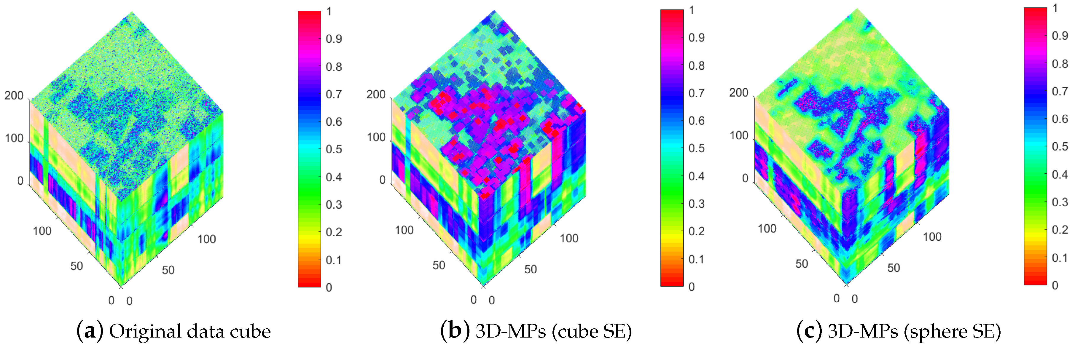
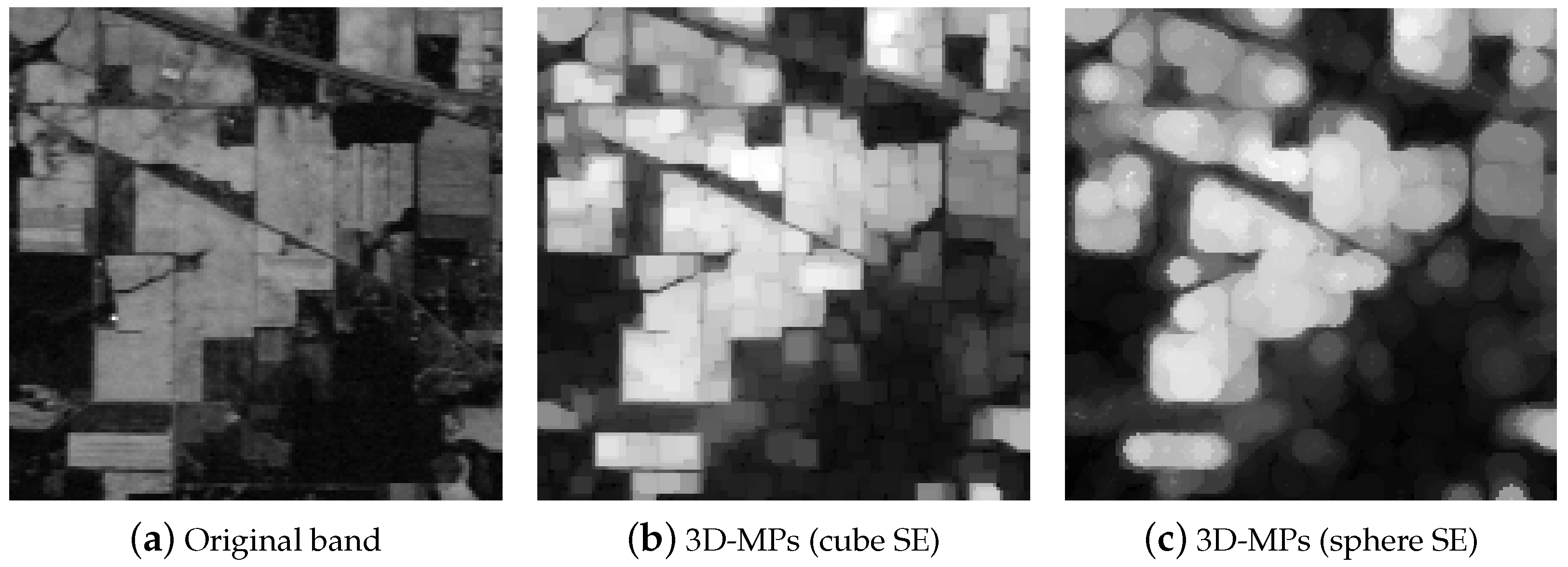
In this section, the experimental results are provided to assess the performance of the 3D-MPs for spectral-spatial feature extraction and the sllMTL for hyperspectral classification. To this end, the 3D-MPs are compared with the “Spec”, EMP and 3D-DWT. The “Spec” utilizes the original spectral features, the EMP can incorporate spatial features, while 3D-DWT and 3D-MPs respect the 3D nature of the HSI and exploit spectral-spatial features. As an example, Figure 7 depicts the 3D-MPs obtained by 3D-opening with both cube and sphere 3D-SEs of side length $L=5$, while Figure 8 plots the 3D-MPs of the 150th band. It can be observed from Figure 7 and Figure 8 that the 3D-MPs highlight the structural characteristics of the HSI cube and provide smoother features in both spectral and spatial domains.

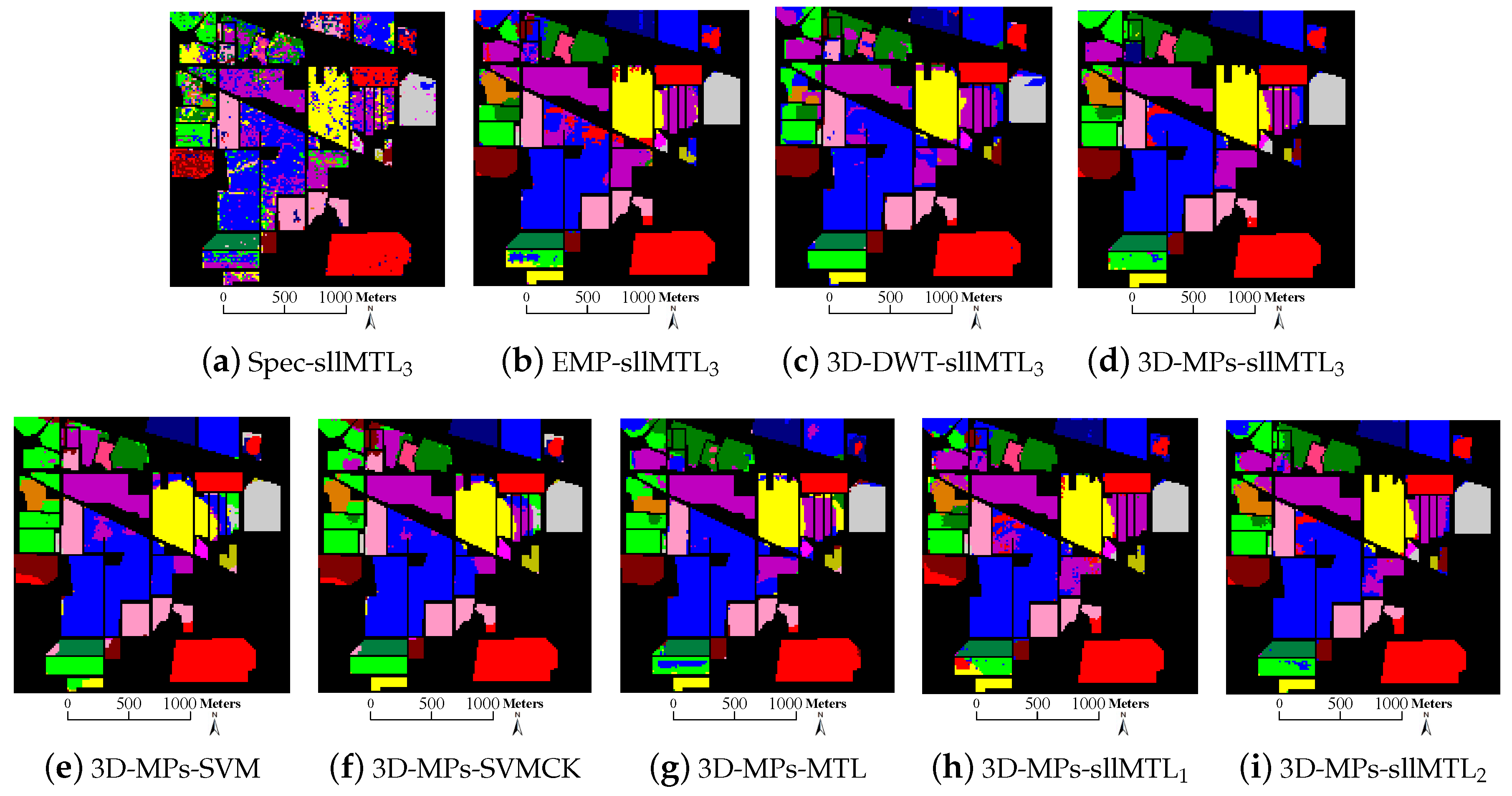
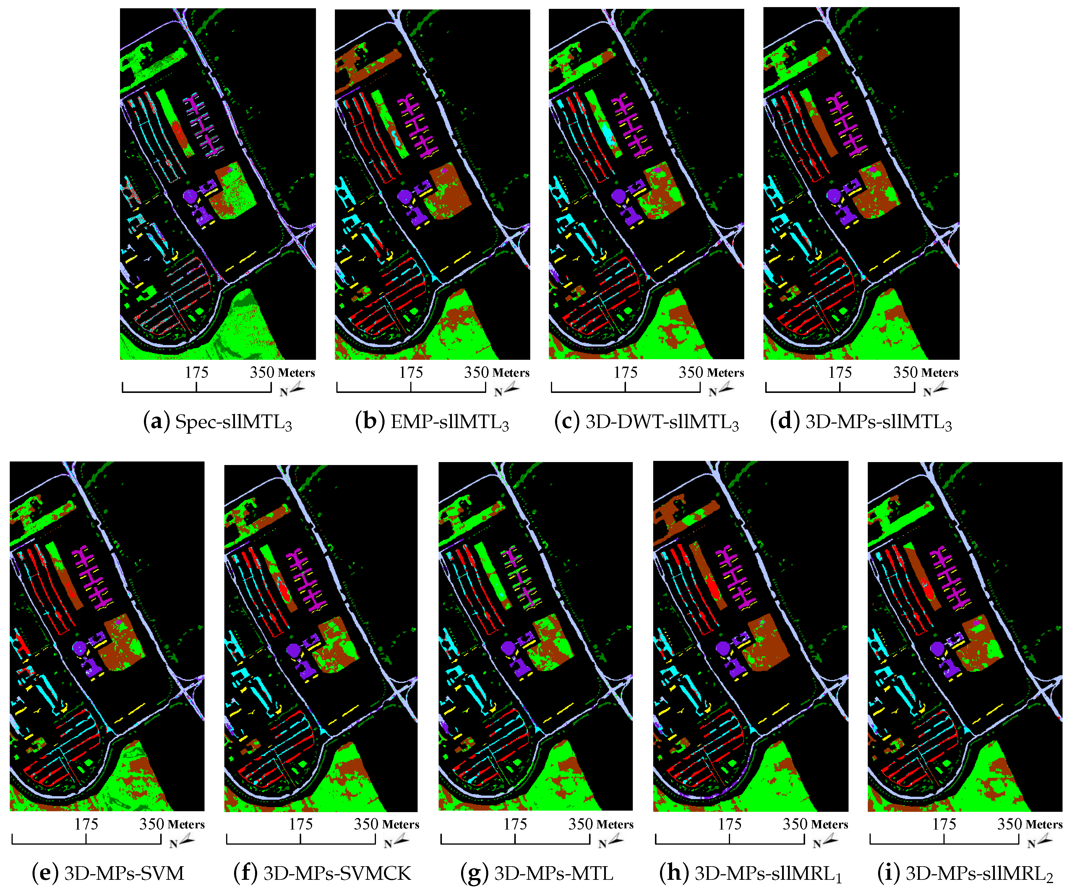
The thematic maps of those methods in a trial are visually reported in Figure 9, Figure 10 and Figure 11, while the detailed average classification accuracies are listed and compared in

Table 4. Classification accuracy (%) of different methods for the Indian Pines data, bold values indicate the best result for a row.

Class	sllMTL${}_3$					3D-MPs
	Spec	EMP	3D-DWT	3D-MPs		SVM	SVMCK	MTL	sllMTL${}_1$	sllMTL${}_2$	sllMTL${}_3$
1	25.38	59.13	63.46	88.46		93.27	93.27	70.77	70.43	73.72	88.46
2	63.90	80.36	82.52	70.68		57.49	61.79	78.27	77.03	74.44	70.68
3	48.85	71.70	70.29	78.42		87.79	85.83	75.61	66.39	73.09	78.42
4	26.54	73.86	74.68	86.15		69.96	76.45	53.46	72.35	73.30	86.15
5	73.70	72.23	73.81	74.59		65.73	67.30	75.94	63.08	72.49	74.59
6	88.44	91.90	92.35	95.81		89.53	90.37	93.25	90.12	92.11	95.81
7	53.75	100.00	100.00	100.00		95.42	100.00	100.00	99.48	100.00	100.00
8	92.98	99.20	99.20	99.17		98.62	98.60	97.19	99.07	99.17	99.17
9	46.67	95.14	93.75	88.89		47.22	80.00	70.56	84.03	87.04	88.89
10	64.06	75.89	76.62	89.98		70.52	75.72	75.82	78.05	82.64	89.98
11	73.24	91.17	91.21	94.35		90.23	90.69	93.78	91.84	96.64	94.35
12	36.39	74.63	74.79	86.33		60.02	63.82	65.85	74.16	74.30	86.33
13	94.16	99.46	99.46	99.52		97.94	98.42	93.21	98.50	98.41	99.52
14	92.58	97.45	97.38	99.53		98.17	98.24	97.66	97.10	99.17	99.53
15	26.81	82.18	83.18	85.11		80.72	83.38	70.19	78.32	84.13	85.11
16	50.00	99.73	99.56	100.00		91.72	95.70	89.57	99.33	98.57	100.00
OA	68.54	85.40	85.84	88.55		81.35	83.11	84.62	84.07	86.93	88.55
AA	59.84	85.25	85.77	89.81		80.90	84.97	81.32	83.71	86.20	89.81
$\kappa$	63.92	83.28	83.79	86.90		78.73	80.76	82.35	81.73	85.00	86.90

,

Table 5. Classification accuracy (%) of different methods for the University of Pavia data, bold values indicate the best result for a row.

Class	sllMTL${}_3$					3D-MPs
	Spec	EMP	3D-DWT	3D-MPs		SVM	SVMCK	MTL	sllMTL${}_1$	sllMTL${}_2$	sllMTL${}_3$
1	68.90	87.91	88.13	92.04		86.62	89.64	87.20	86.07	91.25	92.04
2	77.85	67.59	70.63	69.31		69.31	68.13	73.70	65.15	67.74	69.31
3	51.60	65.60	73.70	82.99		72.46	74.85	73.56	66.22	71.80	82.99
4	86.85	63.94	82.21	97.81		72.06	83.58	80.29	79.96	88.19	97.81
5	72.19	99.93	99.93	79.33		59.70	76.58	60.59	99.85	98.74	79.33
6	38.38	72.94	61.13	76.72		55.90	63.59	58.62	75.98	69.85	76.72
7	89.77	93.08	96.84	93.01		96.69	96.54	91.20	95.34	94.74	93.01
8	41.01	78.79	61.68	74.99		63.25	63.82	69.07	83.41	74.96	74.99
9	59.13	97.99	95.67	99.26		96.09	98.63	96.20	99.47	99.37	99.26
OA	67.79	74.45	74.73	78.62		71.39	73.82	74.71	75.14	76.43	78.62
AA	65.08	80.86	81.10	85.05		74.68	79.48	76.71	83.49	84.07	85.05
$\kappa$	58.03	67.42	67.54	73.02		62.68	66.36	66.74	68.67	70.02	73.02

and

Table 6. Classification accuracy (%) of different methods for the Salinas data, bold values indicate the best result for a row.

Class	sllMTL${}_3$					3D-MPs
	Spec	EMP	3D-DWT	3D-MPs		SVM	SVMCK	MTL	sllMTL${}_1$	sllMTL${}_2$	sllMTL${}_3$
1	97.48	98.54	99.35	99.90		99.45	98.09	98.29	98.64	99.30	99.90
2	99.78	99.16	99.02	100.00		97.97	99.13	99.70	99.54	99.78	100.00
3	98.01	98.11	97.14	99.54		98.77	97.65	98.62	98.21	99.64	99.54
4	98.12	98.99	99.35	99.71		98.70	97.61	99.28	98.70	98.99	99.71
5	98.53	97.81	96.57	98.83		96.57	96.34	97.51	96.83	98.30	98.83
6	99.95	99.95	99.13	99.97		99.16	98.72	99.72	99.92	99.92	99.97
7	99.72	98.50	99.41	99.86		95.96	99.27	99.63	99.69	99.77	99.86
8	89.56	88.19	91.49	93.85		83.82	87.42	91.76	90.10	93.37	93.85
9	99.45	99.67	99.25	99.90		99.59	99.09	99.35	99.54	99.79	99.90
10	89.65	95.10	93.93	98.34		87.70	92.70	96.21	96.09	95.93	98.34
11	91.49	98.01	94.99	99.62		90.26	95.65	88.55	92.90	96.78	99.62
12	99.58	99.42	99.79	100.00		99.63	99.58	99.84	99.84	99.79	100.00
13	98.45	98.34	99.12	99.45		97.90	98.12	98.23	94.81	99.45	99.45
14	94.81	95.85	97.26	99.34		96.79	93.67	93.86	97.92	97.54	99.34
15	57.05	85.24	83.16	86.46		82.34	81.26	80.93	81.14	81.42	86.46
16	98.04	97.26	98.49	99.22		96.98	96.48	98.27	98.64	97.54	99.22
OA	90.67	94.54	94.80	96.64		92.33	93.34	94.66	94.43	95.46	96.64
AA	94.35	96.76	96.71	98.37		95.10	95.67	96.24	96.39	97.33	98.37
$\kappa$	89.57	93.93	94.20	96.25		91.45	92.59	94.05	93.79	94.94	96.25

. A few observations can be made based on the above-mentioned experimental results.

It can be first seen that, the original “Spec”, which is based only on spectral characteristics, provides poor classification results compared with other methods. For instance, the OA of SVM in the Indian Pines data (see Table 4) is 16.86%, 17.30% and 20.01% lower than those of the EMP, 3D-DWT and 3D-MPs, respectively. As shown in Figure 9, the Spec-sllMTL${}_3$ produces much more “salt-and-pepper” phenomenon than its counterparts. Similar properties can also be found in the University of Pavia data and the Salinas data. Note that the “Spec” utilizes the original spectral features without a spatial prior, it is not hard to infer that the spatial information can be utilized to alleviate the spectral variations and stabilize the pixel-based features. Therefore, the above-mentioned phenomena stress yet again the importance of spatial information for HSI classification.

Second, the 3D-based feature extraction methods (i.e., 3D-DWT and 3D-MPs) achieve comparable or better performance than the 2D-based one (i.e., EMP). For instance, as observed from Table 5, the OA, AA and $\kappa$ of 3D-DWT are slightly better than the EMP, while the OA, AA and $\kappa$ of 3D-MPs are 4.17%, 4.19%, 5.60% higher than the EMP, respectively. The classification results of the 3D-DWT and 3D-MPs are also comparable or better than the EMP in Table 4 and Table 6. The reason for good results of 3D-DWT and 3D-MPs-based feature extraction methods is that they can respect the 3D nature of the HSI cube by taking the HSI cube as a whole entity to extract the spectral-spatial features.

Third, the 3D-MPs yields the best classification performance in all the feature extraction methods by fixing the sllMTL${}_3$ as classifier. For instance, in the Indian Pines data (see Table 4), the OA of 3D-MPs is 20.01%, 3.15% and 2.71% higher than those of the “Spec”, EMP and 3D-DWT, respectively. In the University of Pavia data (see Table 5), the OA of 3D-MPs is also 10.83%, 4.17% and 3.89% higher than those of the “Spec”, EMP and 3D-DWT, respectively. In the Salinas data (see Table 6), the OA of 3D-MPs is 5.97%, 2.10% and 1.84% higher than other feature extraction methods. Similarly, the AA and $\kappa$ of the 3D-MPs are also much higher than its counterparts on the three HSI datasets. It demonstrates that multiple features obtained by varying the shapes and sizes of SEs can offer additional complementary information, and thus, effectively improve the performance of hyperspectral classification.

Fourth, the classification results of the SVM are inferior to other ones. For instance, it can be observed from Table 4 that the OA of SVM is about 2% to 7% lower than other classifiers (i.e., SVMCK, MTL, sllMTL${}_1$, sllMTL${}_2$ and sllMTL${}_3$), the AA (or $\kappa$) of SVM is also about 0.4% to 9% (or 2% to 8%) lower than its competitors. It is notable that the classification results of the University of Pavia data (see Table 5) and the Salinas data (see Table 6) also yield similar properties. This is due to the fact that the SVM cannot able to cope with the multiple-feature-based scenario but simple stacks the multiple 3D-MPs together to generate a single cube, while the other methods can make full use of the multiple 3D-MPs features by taking each 3D-MPs cube as the feature of a task.

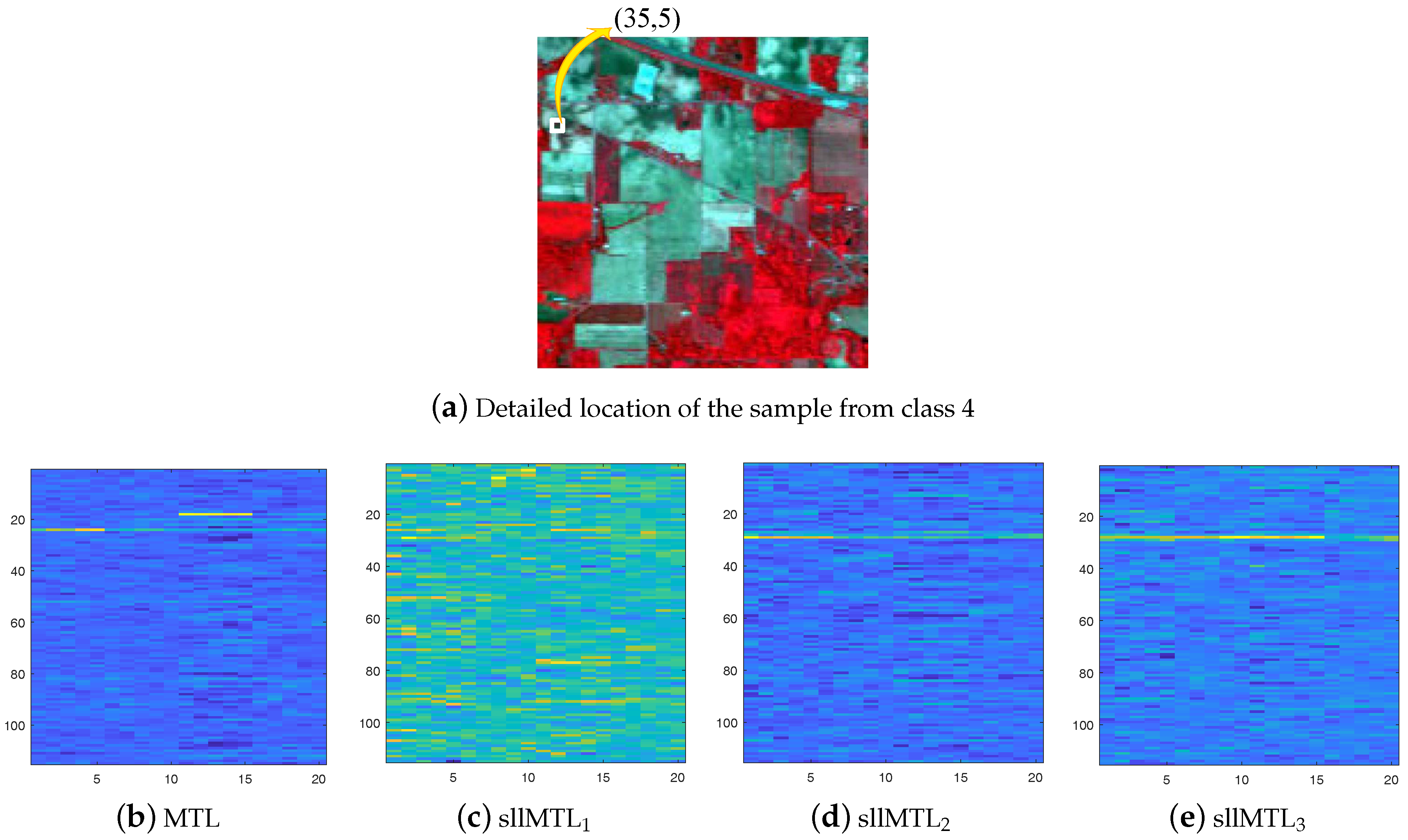
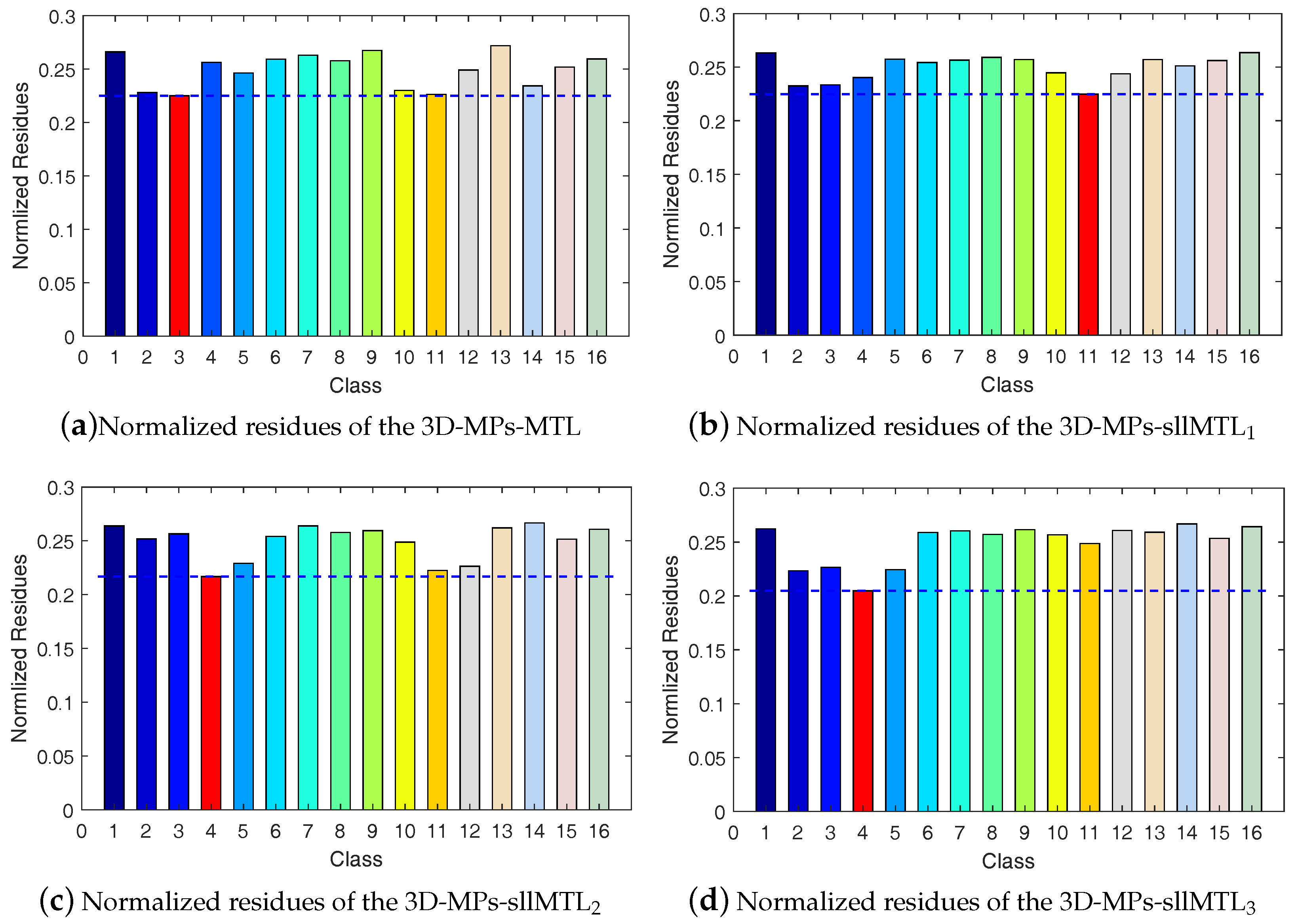
Fifth, we compare the multitask-based classifiers (i.e., MTL, sllMTL${}_1$, sllMTL${}_2$ and sllMTL${}_3$) by utilizing the 3D-MPs-based features. To provide intuitive insight, the coefficient matrices of a test sample from class 4 (i.e., corn) located at (35,5) in the Indian Pines data are compared in Figure 12. The x-axis labels the task number and the y-axis labels the representation number. We can see from Figure 12 that, for an instance in a certain class of data, a distinctive training feature is active in the sllMTL${}_2$ and sllMTL${}_3$. The joint sparse and low-rank constraints in the sllMTL${}_2$ and sllMTL${}_3$ can effectively capture the task specificity and relatedness, and thus alleviate the misclassification problem. The normalized residues of the same sample from class 4 (i.e., corn) located at (35,5) are plotted in Figure 13, from which one can observe that, by utilizing the 3D-MPs features, the sllMTL${}_2$ and sllMTL${}_3$ yield more accurate classification results than the MTL and sllMTL${}_1$. Moreover, it is shown in Table 4, Table 5 and Table 6 that the sllMTL${}_2$ and sllMTL${}_3$ outperform the MTL and sllMTL${}_1$, and the sllMTL${}_3$ performs much better than the sllMTL${}_2$ since a Laplacian-like regularization is added in the sllMTL${}_3$ to take full advantage of the label information of training samples. In addition, as displayed in Figure 9, Figure 10 and Figure 11, the classification maps of sllMTL${}_3$ are more close to the ground truth (see Figure 4a, Figure 5b and Figure 6b) than other methods.

Finally, it is worthwhile to note that the proposed method is much better than those in previous work (e.g., [17,34]). Although we use the same hyperspectral datasets as [17,34], the number of training and test samples are completely different. For instance, in the Indian Pines data, around 10% of the labeled samples are chosen for training in [17], while only 1% samples per class are selected as training samples in this paper. Therefore, it is not very surprising to see that the OA of our proposed method is much lower than the results shown in Table 2 of [17]. As can be seen in Figure 5 of [17], the OA is lower than 75% when only 1% labeled samples in each class are chosen as training samples, while the OA of 3D-MPs-sllMTL${}_3$ achieves to 88.55% with the same number of training samples. Similarly, in the University of Pavia data, the number of training samples is 3921 in [34], while very limited training samples (1% samples from the available 3921 training samples are chosen for training, i.e., about 39 samples in total) are chosen in this paper. It is observed from Table 5 that the classification performance of 3D-MPs is better than the EMP with the same classifier.

5. Discussion

5.1. Statistical Significance Analysis of the Results

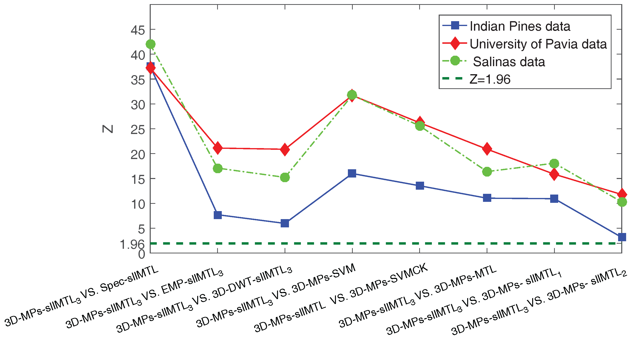
To discuss whether the proposed method significantly outperforms its counterparts, we apply the McNemar’s test to evaluate the statistical significance in accuracy improvement. The McNermar’s test is a non-parametric test based upon the standardized normal test statistic

$$Z=\frac{f_{12}-f_{21}}{\sqrt{f_{12}+f_{21}}}$$

(17)

where $f_{ij}$ indicates the number of samples classified correctly by the classifier i but incorrectly by the classifier j. This test allows two methods to be compared. In this paper, we compare the 3D-MPs-sllMTL${}_3$ with the other methods one by one. If the absolute of the McNemar’s value Z is greater than 1.96 (i.e., $\left|Z\right|>1.96$), the difference in accuracy between the ith and jth classifiers is considered statistically significant at the 5% level of significance. The average McNemar’s values Z of the proposed method and other methods by utilizing the afore-mentioned three experimental datasets are depicted in Figure 14. It is clearly shown in Figure 14 that the Z is larger than 1.96 in all cases, and therefore, the 3D-MPs-sllMTL${}_3$ performs significantly better than the other methods according to the McNemar’s test.

5.2. Sensitivity Analysis of the Parameters

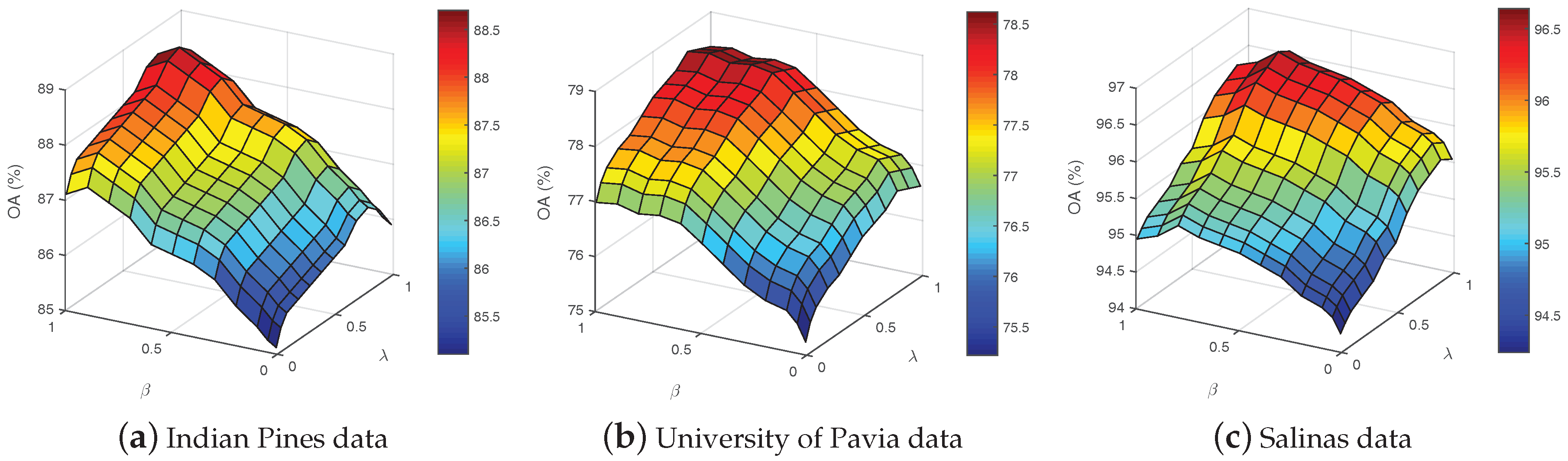
Another important issue is to discuss the sensitivity of the parameters in the proposed 3D-MPs-sllMTL${}_3$. There are two key parameters in the 3D-MPs-sllMTL${}_3$: $\lambda$ and $\beta$. The impacts of the parameters $\lambda$ and $\beta$ are shown in Figure 15, whose x-axis and y-axis are the value ranges of the corresponding parameters and the z-axis denotes the OA (%) of various hyperspectral datasets. It can be seen from Figure 15 that the classification accuracies for the three datasets generally improve slowly as the parameters $\lambda$ and $\beta$ increase, and then, begin to decrease after obtaining the maximum values. When the parameters $\lambda$ and $\beta$ are very small, the low-rank constraint term will dominate the optimization process and the sparse and Laplacian-like regularizations will be weakened. The influence of the sparse and Laplacian-like regularizations will become strong with the increase of $\lambda$ and $\beta$. Based on the above analysis, it is better to make a tradeoff among the three constraints so as to achieve satisfactory classification performance.

5.3. Influence Analysis of the 3D-SEs

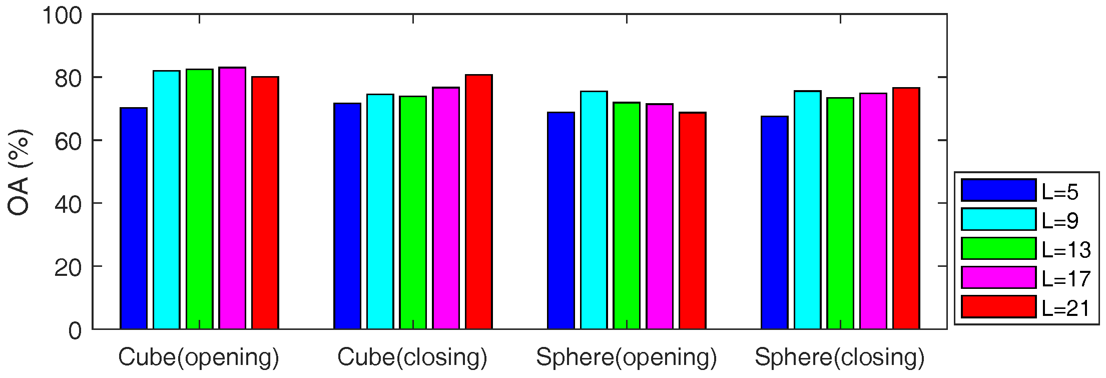
Note that one can extract different structure features of the HSI by applying a series of 3D-SEs, it is interesting to analyze the influence of the 3D-SEs with different shapes and sizes. As an example, we discuss the influence of the 3D-SEs in the Indian Pines data. Both cube and sphere shapes with side length $L=5,9,13,17$ and 21 are adopted in the experiments. We set $K=1$ in the sllMTL${}_3$ and analyze the influence of the 3D-SEs by classifying each 3D-MP feature separately. The classification results of different 3D-MPs is shown in Figure 16, from which we can observe that the sphere(closing) with $L=5$ provides the lowest classification accuracy, while cube(opening) with $L=17$ achieves the highest classification accuracy among all the 3D-MPs. However, it is shown in Table 4 that the combination of multiple 3D-MPs gives much better performance than using each 3D-MP feature separately. The reason is that a single 3D-MP can only reflect the characteristic of the HSI in one aspect, while multiple features can represent the characteristic of the HSI more effectively from different perspectives.

6. Conclusions

In this paper, we have proposed a 3D-MPs-based MTL framework, namely, 3D-MPs-sllMTL, for hyperspectral imagery classification. On the one hand, the 3D-opening and 3D-closing operators are applied for feature extraction of the HSI cubes. Multiple SEs with different shapes and sizes are used to extract the spectral-spatial features from different aspects. Comparing against the vector/image-based methods in the literature, the proposed 3D-MPs-based method respects the 3D nature of the HSI by taking the HSI cube as a whole entity. On the other hand, the sllMTL method is proposed in this paper to exploit the joint sparse and low-rank structures by taking each 3D-MP as features of a specific task. Comparing against the existing MTL methods, the proposed sllMTL can capture both specificities and shared factors of the tasks by adopting the joint sparse and low-rank constraints. The Laplacian-like regularization can also improve the classification performance further by making full use of the class label information. We have validated the superiority of the 3D-MPs-sllMTL approach on three benchmark hyperspectral datasets and compared our method with a number of alternatives, i.e., the original “Spec”, EMP, 3D-DWT, SVM, SVMCK and MTL. The experimental results consistently demonstrate the effectiveness of the proposed method. Quantitatively, by utilizing the 3D-MPs features, the OA of sllMTL${}_3$ is at least about 4%, 3% and 2% higher than the SVM, SVMCK and MTL, respectively. By utilizing the sllMTL${}_3$, the OA of 3D-MPs is at least about 6%, 2% and 2% higher than the “Spec”, EMP and 3D-DWT, respectively. Note that the sllMTL considers an equal contribution for any 3D-MPs-based features in the classification process, a future research direction is to investigate the importance of different features by assigning different weights to the features. Extending the sllMTL to its kernel versions is also a promising research topic for further improving the classification performance. Moreover, as to other kinds of images (e.g., the sequence of the 2D images or medical images), we can also take them as 3D cubes, whose 3D-MPs features can be extracted by the 3D MM. However, the sllMTL cannot be directly used for classification of those images because a pixel in those images usually comes from different classes. One should extract and arrange the features from the same class together before applying the sllMTL. Therefore, applying the proposed method to classify other images (e.g., the sequence of the 2D images or medical images) is also an interesting area of future work.

References

- Guanter, L.; Kaufmann, H.; Segl, K.; Foerster, S.; Rogass, C.; Chabrillat, S.; Kuester, T.; Hollstein, A.; Rossner, G.; Chlebek, C.; et al. The EnMAP spaceborne imaging spectroscopy mission for Earth Observation. Remote Sens. 2015, 7, 8830–8857. [Google Scholar] [CrossRef] [Green Version]
- Angelliaume, S.; Ceamanos, X.; Viallefont-Robinet, F.; Baqué, R.; Déliot, P.; Miegebielle, V. Hyperspectral and Radar airborne imagery over controlled release of oil at sea. Sensors 2017, 17, 1772. [Google Scholar] [CrossRef] [PubMed]
- Fu, Y.; Zhao, C.; Wang, J.; Jia, X.; Yang, G.; Song, X.; Feng, H. An improved combination of spectral and spatial features for vegetation classification in hyperspectral images. Remote Sens. 2017, 9, 261. [Google Scholar] [CrossRef]
- Schneider, S.; Murphy, R.J.; Melkumyan, A. Evaluating the performance of a new classifier-the GP-OAD: A comparison with existing methods for classifying rock type and mineralogy from hyperspectral imagery. ISPRS J. Photogramm. Remote Sens. 2014, 98, 145–156. [Google Scholar] [CrossRef]
- Sun, B.; Kang, X.; Li, S.; Benediktsson, J.A. Random-walker-based collaborative learning for hyperspectral image classification. IEEE Trans. Geosci. Remote Sens. 2017, 55, 212–222. [Google Scholar] [CrossRef]
- Kang, X.; Xiang, X.; Li, S.; Benediktsson, J.A. PCA-based edge-preserving features for hyperspectral image classification. IEEE Trans. Geosci. Remote Sens. 2017, 55, 7140–7151. [Google Scholar] [CrossRef]
- Gao, L.; Zhao, B.; Jia, X.; Liao, W.; Zhang, B. Optimized kernel minimum noise fraction transformation for hyperspectral image classification. Remote Sens. 2017, 9, 548. [Google Scholar] [CrossRef]
- Zhong, Y.; Jia, T.; Zhao, J.; Wang, X.; Jin, S. Spatial-spectral-emissivity land-cover classification fusing visible and thermal infrared hyperspectral imagery. Remote Sens. 2017, 9, 910. [Google Scholar] [CrossRef]
- Vapnik, V. The Nature of Statistical Learning Theory; Springer Science & Business Media: New York, NY, USA, 2013. [Google Scholar]
- Kuo, B.C.; Ho, H.H.; Li, C.H.; Hung, C.C.; Taur, J.S. A kernel-based feature selection method for SVM with RBF kernel for hyperspectral image classification. IEEE J. Sel. Top. Appl. Earth Obs. Remote Sens. 2014, 7, 317–326. [Google Scholar]
- Camps-Valls, G.; Gomez-Chova, L.; Muñoz-Marí, J.; Vila-Francés, J.; Calpe-Maravilla, J. Composite kernels for hyperspectral image classification. IEEE Geosci. Remote Sens. Lett. 2006, 3, 93–97. [Google Scholar] [CrossRef]
- Gu, Y.; Wang, C.; You, D.; Zhang, Y.; Wang, S.; Zhang, Y. Representative multiple kernel learning for classification in hyperspectral imagery. IEEE Trans. Geosci. Remote Sens. 2012, 50, 2852–2865. [Google Scholar] [CrossRef]
- Gurram, P.; Kwon, H. Sparse kernel-based ensemble learning with fully optimized kernel parameters for hyperspectral classification problems. IEEE Trans. Geosci. Remote Sens. 2013, 51, 787–802. [Google Scholar] [CrossRef]
- Maulik, U.; Chakraborty, D. Learning with transductive SVM for semisupervised pixel classification of remote sensing imagery. ISPRS J. Photogramm. Remote Sens. 2013, 77, 66–78. [Google Scholar] [CrossRef]
- Wang, L.; Hao, S.; Wang, Q.; Wang, Y. Semi-supervised classification for hyperspectral imagery based on spatial-spectral label propagation. ISPRS J. Photogramm. Remote Sens. 2014, 97, 123–137. [Google Scholar] [CrossRef]
- Wright, J.; Yang, A.; Ganesh, A.; Sastry, S.; Ma, Y. Robust face recognition via sparse representation. IEEE Trans. Pattern Anal. Mach. Intell. 2009, 31, 210–227. [Google Scholar] [CrossRef] [PubMed]
- Chen, Y.; Nasrabadi, N.M.; Tran, T.D. Hyperspectral image classification using dictionary-based sparse representation. IEEE Trans. Geosci. Remote Sens. 2011, 49, 3973–3985. [Google Scholar] [CrossRef]
- Chen, Y.; Nasrabadi, N.M.; Tran, T.D. Hyperspectral image classification via kernel sparse representation. IEEE Trans. Geosci. Remote Sens. 2013, 51, 217–231. [Google Scholar] [CrossRef]
- Zhang, H.; Li, J.; Huang, Y.; Zhang, L. A nonlocal weighted joint sparse representation classification method for hyperspectral imagery. IEEE J. Sel. Top. Appl. Earth Obs. Remote Sens. 2014, 7, 2056–2065. [Google Scholar] [CrossRef]
- Srinivas, U.; Suo, Y.; Dao, M.; Monga, V.; Tran, T.D. Structured sparse priors for image classification. IEEE Trans. Image Process. 2015, 24, 1763–1776. [Google Scholar] [CrossRef] [PubMed]
- Dao, M.; Nguyen, N.H.; Nasrabadi, N.M.; Tran, T.D. Collaborative multi-sensor classification via sparsity-based representation. IEEE Trans. Signal Process. 2016, 64, 2400–2415. [Google Scholar] [CrossRef]
- Bian, X.; Chen, C.; Xu, Y.; Du, Q. Robust hyperspectral image classification by multi-layer spatial-spectral sparse representations. Remote Sens. 2016, 8, 985. [Google Scholar] [CrossRef]
- Zhang, S.; Li, S.; Fu, W.; Fang, L. Multiscale superpixel-based sparse representation for hyperspectral image classification. Remote Sens. 2017, 9, 139. [Google Scholar] [CrossRef]
- Xue, Z.; Du, P.; Su, H.; Zhou, S. Discriminative sparse representation for hyperspectral image classification: a semi-supervised perspective. Remote Sens. 2017, 9, 386. [Google Scholar] [CrossRef]
- Dao, M.; Kwan, C.; Koperski, K.; Marchisio, G. A joint sparsity approach to tunnel activity monitoring using high resolution satellite images. In Proceedings of the IEEE 8th Annual Ubiquitous Computing, Electronics and Mobile Communication Conference (UEMCON), New York, NY, USA, 19–21 October 2017; pp. 322–328. [Google Scholar]
- Ul Haq, Q.S.; Tao, L.; Sun, F.; Yang, S. A fast and robust sparse approach for hyperspectral data classification using a few labeled samples. IEEE Trans. Geosci. Remote Sens. 2012, 50, 2287–2302. [Google Scholar] [CrossRef]
- He, Z.; Wang, Q.; Shen, Y.; Sun, M. Kernel sparse multitask learning for hyperspectral image classification with empirical mode decomposition and morphological wavelet-based features. IEEE Trans. Geosci. Remote Sens. 2014, 52, 5150–5163. [Google Scholar]
- Li, J.; Zhang, H.; Zhang, L.; Huang, X.; Zhang, L. Joint collaborative representation with multitask learning for hyperspectral image classification. IEEE Trans. Geosci. Remote Sens. 2014, 52, 5923–5936. [Google Scholar] [CrossRef]
- Li, J.; Zhang, H.; Zhang, L. A nonlinear multiple feature learning classifier for hyperspectral images with limited training samples. IEEE J. Sel. Topics Appl. Earth Observ. Remote Sens. 2015, 8, 2728–2738. [Google Scholar] [CrossRef]
- Zhang, Y.; Wu, K.; Du, B.; Zhang, L.; Hu, X. Hyperspectral target detection via adaptive joint sparse representation and multi-task learning with locality information. Remote Sens. 2017, 9, 482. [Google Scholar] [CrossRef]
- Jia, S.; Deng, B.; Zhu, J.; Jia, X.; Li, Q. Superpixel-based multitask learning framework for hyperspectral image classification. IEEE Trans. Geosci. Remote Sens. 2017, 55, 2575–2588. [Google Scholar] [CrossRef]
- Kang, X.; Li, S.; Benediktsson, J.A. Spectral-spatial hyperspectral image classification with edge-preserving filtering. IEEE Trans. Geosci. Remote Sens. 2014, 52, 2666–2677. [Google Scholar] [CrossRef]
- Benediktsson, J.; Palmason, J.; Sveinsson, J. Classification of hyperspectral data from urban areas based on extended morphological profiles. IEEE Trans. Geosci. Remote Sens. 2005, 43, 480–491. [Google Scholar] [CrossRef]
- Fauvel, M.; Tarabalka, Y.; Benediktsson, J.A.; Chanussot, J.; Tilton, J.C. Advances in spectral-spatial classification of hyperspectral images. Proc. IEEE 2013, 101, 652–675. [Google Scholar] [CrossRef]
- Hou, B.; Huang, T.; Jiao, L. Spectral-spatial classification of hyperspectral data using 3-D morphological profile. IEEE Geosci. Remote Sens. Lett. 2015, 12, 2364–2368. [Google Scholar]
- Lin, Z.; Liu, R.; Su, Z. Linearized alternating direction method with adaptive penalty for low-rank representation. In Advances in Neural Information Processing Systems 24 (NIPS 2011); Curran Associates, Inc.: Granada, Spain, 2011; pp. 612–620. [Google Scholar]
- Qian, Y.; Ye, M.; Zhou, J. Hyperspectral image classification based on structured sparse logistic regression and three-dimensional wavelet texture features. IEEE Trans. Geosci. Remote Sens. 2013, 51, 2276–2291. [Google Scholar] [CrossRef]
Figure 1.
Schematic illustration of the proposed HSI classification method.
Figure 2.
3D-SEs examples with various shapes (e.g., cube, sphere) and sizes (e.g., side length (L) is set to 3, 5 and 7). (a–c) are spheres with different sizes, and (d–f) are cubes with different sizes
Figure 3.
TheW used in (a) Indian Pines data, (b) University of Pavia data and (c) Salinas data.
Figure 4.
Indian Pines data. (a) Three-band false color composite and (b) ground truth data with 16 classes.
Figure 5.
University of Pavia data. (a) Three-band false color composite, (b) ground truth data with 9 classes and (c) available training samples.
Figure 6.
Salinas data. (a) Three-band false color composite and (b) ground truth data with 16 classes.
Figure 7.
3D-MPs 3D-MPs obtained by 3D-opening with both cube and sphere SEs of side length L = 5. (a) is the original Indian Pines data, (b) is the 3D-MPs obtained by the cube SE, and (c) is the 3D-MPs obtained by the sphere SE.(sphere SE)
Figure 8.
Spatial scenes of the 150th band. (a) is chosen from the original Indian Pines data, and (b,c) are chosen from the 3D-MPs.
Figure 9.
Classification maps of the Indian Pines data obtained by different methods.
Figure 10.
Classification maps of the University of Pavia data obtained by different methods.
Figure 11.
Classification maps of the Salinas data obtained by different methods.
Figure 12.
The coefficient matrices of a test sample from class 4 (i.e., corn) located at (35,5) in the Indian Pines data for (b) MTL, (c) sllMTL1, (d) sllMTL2, and (e) sllMTL3. The x-axis labels the task number and the y-axis labels the representation number.
Figure 13.
Normalized residues of a sample from class 4 (i.e., corn) located at (35,5). (a–d) are the normalized residues of the 3D-MPs-MTL, 3D-MPs-sllMTL1, 3D-MPs-sllMTL2, and 3D-MPs-sllMTL3, respectively.
Figure 14.
McNemar’s test between 3D-MPs-sllMTL and other methods.
Figure 15.
The impact of parameters λ and β on the OA in (a) Indian Pines data, (b) University of Pavia data and (c) Salinas data.
Figure 16.
Classification results the sllMTL by using different 3D-MPs.