The Correlation Coefficient as a Simple Tool for the Localization of Errors in Spectroscopic Imaging Data


1
Flight Research Laboratory, National Research Council of Canada, Ottawa, ON K1A 0R6, Canada
2
Applied Remote Sensing Laboratory, Department of Geography, McGill University, Montréal, QC H3A 0B9, Canada
*
Author to whom correspondence should be addressed.
Remote Sens. 2018, 10(2), 231; https://doi.org/10.3390/rs10020231
Submission received: 1 December 2017
/
Revised: 24 January 2018
/
Accepted: 29 January 2018
/
Published: 2 February 2018
(This article belongs to the Section Remote Sensing Image Processing)
Abstract
:The correlation coefficient (CC) was substantiated as a simple, yet robust statistical tool in the quality assessment of hyperspectral imaging (HSI) data. The sensitivity of the metric was also characterized with respect to artificially-induced errors. The CC was found to be sensitive to spectral shifts and single feature modifications in hyperspectral ground data despite the high, artificially-induced, signal-to-noise ratio (SNR) of 100:1. The study evaluated eight airborne hyperspectral images that varied in acquisition spectrometer, acquisition date and processing methodology. For each image, we identified a uniform ground target region of interest (ROI) that was comprised of a single asphalt road pixel from each column within the sensor field-of-view (FOV). A CC was calculated between the spectra from each of the pixels in the ROI and the data from the center pixel. Potential errors were located by reductions in the CCs below a designated threshold, which was derived from the results of the sensitivity tests. The spectral range associated with each error was established using a windowing technique where the CCs were recalculated after removing the spectral data within various windows. Errors were isolated in the spectral window that removed the previously-identified reductions in the CCs. Finer errors were detected by calculating the CCs across the ROI in the spectral range surrounding various atmospheric absorption features. Despite only observing deviations in the CCs from the 3rd–6th decimal places, non-trivial errors were detected in the imagery. An error was detected within a single band of the shortwave infrared imagery. Errors were also observed throughout the visible-near-infrared imagery, especially in the blue end. With this methodology, it was possible to immediately gauge the spectral consistency of the HSI data across the FOV. Consequently, the effectiveness of various processing methodologies and the spectral consistency of the imaging spectrometers themselves could be studied. Overall, the research highlights the utility of the CC as a simple, low monetary cost, analytical tool for the localization of errors in spectroscopic imaging data.

1. Introduction
In imaging spectroscopy, contiguous narrow-band spectrographic information is collected for each spatial pixel in an imaging system. The technology is presently synonymous with hyperspectral imaging (HSI) and is commonly implemented within the discipline of remote sensing to characterize the physical and chemical properties of observed materials. This is preformed via spectroscopic and spatial analysis methodologies [1]. Imaging spectroscopy technologies have shown their utility in numerous remote sensing applications in geology [2,3,4], defense [5,6], agriculture [7,8,9], forestry [10,11,12], oceanography [13,14,15], forensics [16,17,18] and ecology [15,19,20], among others. In theory, spectrographic imaging data are spectrally and spatially piece-wise smooth; neighboring locations and wavelengths are well-correlated due to the high spatial-spectral resolution allowed by the narrow band criterion [21,22].
With such an abundance of information, the processing and analysis of HSI data are not trivial. Relevant spectral signatures are often difficult to identify, especially given the presence of signal noise, which further impedes information extraction [23]. Spatial and spectral correlations can be exploited to aid in the analysis of imaging spectroscopy data with a correlation metric. The Pearson product-moment correlation coefficient (CC) is one of the simplest statistical tools that has been widely implemented to measure levels of correlation [24].
The CC is a measure of linear association between two variables. It is formally given [24] by Equation (1):
where , , , represent the two variables of interest and their means, respectively. In mathematical terms, the CC represents the sum of the centered and normalized cross-product of x and y [24]. Each variable is centered by removing its mean. The denominator normalizes the numerator by the variance of the studied variables. Using the Cauchy–Swartz inequality, it can be shown [24] that the numerator is always less than or equal to the denominator. Therefore, the value of the CC is bounded between −1 and 1. The boundary values represent a perfect linear correlation between and . A value of zero corresponds to no linear correlation between the variables. Values greater than zero indicate a positive correlation between the variables of interest; the opposite is true for values less than zero. The CC is a useful descriptive measure of correlation since its value does not depend on the scales of measurement for the studied variables [24]. It is important to note that the calculation of the CC is not limited by any statistical assumptions; however, its value as an input to other statistical metrics may need to conform to certain restraints (e.g., normally-distributed data).
To date, the CC has been widely implemented to investigate spectrographic imaging data [11,25,26,27,28,29,30,31,32,33,34,35]. In these efforts, the literature has concentrated on applying the statistical tool to establish bands that linearly associate with quantifiable physical and chemical properties. Exploiting the linear relation, this method of band selection has been used to create and improve predictive models that associate hyperspectral data with useful parameters [11,25,27,29,30,31,32,34,35]. For example, Peng et al. [11] applied the CC to establish bands that strongly correlate with forest leaf area index, improving predictive models at the landscape level. To a lesser extent, the CC has been applied for the purposes of data reduction and correction [25,28,33,36]. In 2011, Richter et al. [33] outlined a corrective method for HSI data that relied, in part, on the CC. The correction accounted for the effects of the spectral smile, a spectral non-uniformity in the cross-track direction that is caused by the optical design of the spectrometer and results in per pixel changes in wavelength registration across the field-of-view (FOV) [33]. In the study, the CC was used to measure uniformity levels across the FOV, indirectly assessing the effects of the spectral smile defect. A corrective solution was selected by maximizing this metric. From this application, the CC was shown to be a useful tool in the assessment of HSI data. Following this example, the CC can be used for the detection and quantification of other errors. This was exemplified by Tanabe and Saeki [26], who rigorously quantified the sensitivity of the CC to spectral shifts in infrared spectra. Such research was fundamental to the application of the CC for error detection in infrared spectroscopy. Unfortunately, the findings were somewhat limited in their application to hyperspectral remote sensing as the study was conducted in an ideal environment with a laboratory-grade spectrometer. Earth observation (EO) remotely-sensed measurements are most often collected with airborne spectrometers under less than the ideal conditions. Before the CC can be confidently applied to hyperspectral EO data, the sensitivity of the tool needs to be characterized with respect to various potential errors and noise levels.
The purpose of this study was to use the CC to develop an easy to implement methodology to detect issues with HSI data. The methodology was intended explicitly for the detection of errors, not for the identification of their origin. Although other error detection methodologies exist (e.g., [37,38,39,40]), they can be expensive to implement and rely on a higher level of mathematical understanding. To develop a novel method, the CC was first characterized with respect to artificially-induced errors in ground data. Afterwards, this information was applied to locate the spatial location and spectral bands associated with errors in real HSI data. The overall objective of this study was to substantiate the CC metric as a low monetary cost, robust and simple statistical tool in the quality assessment of EO HSI data through the detection of errors.
2. Materials and Methods
2.1. In-Situ Ground Hyperspectral Data
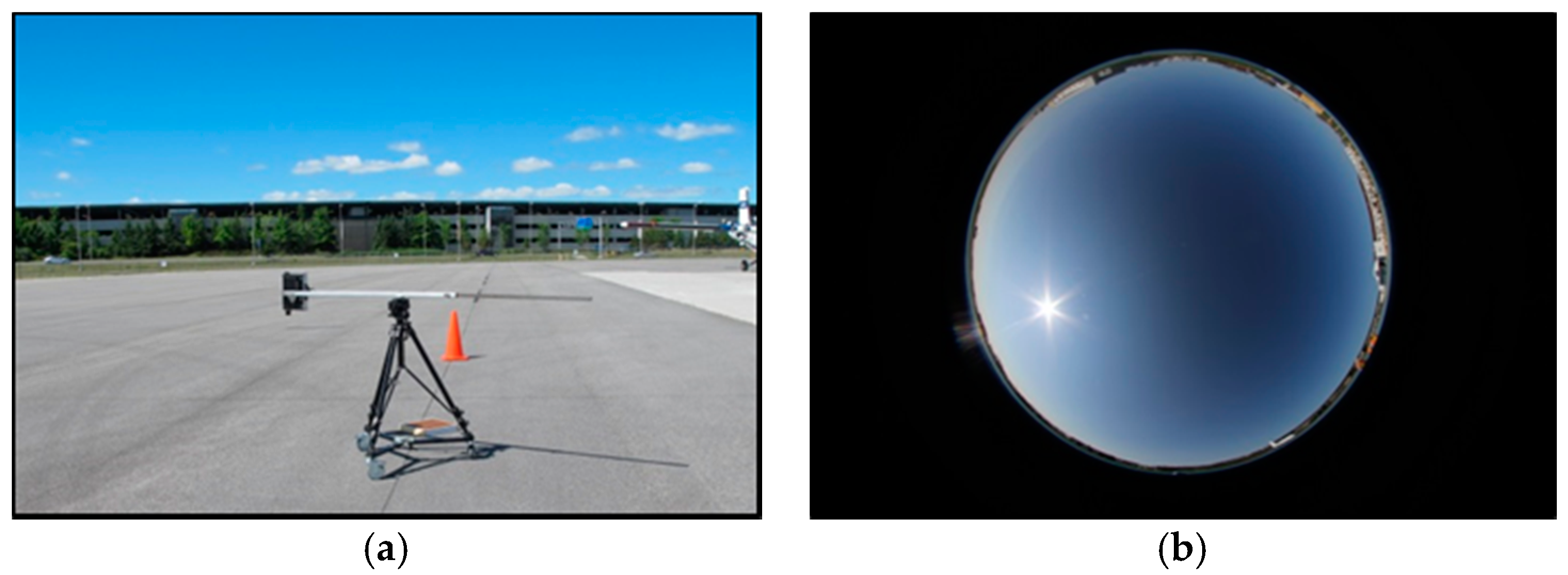
In-situ hyperspectral radiance measurements were collected on 23 June 2016, from 16:54:19 to 17:00:36 GMT with a Spectra Vista Corporation (Poughkeepsie, NY, USA) HR-1024i ground spectrometer at the Flight Research Laboratory of the National Research Council of Canada (NRC) under stable illumination conditions (Figure 1). The HR-1024i is a solid-state device that collects radiance data in a circular FOV. The device collects spectral data over 1024 spectral bands, which are non-uniformly distributed between 350 and 2500 nm using three independent detectors: a single 512-chanel silicon photodiode array and two 256-channel indium gallium arsenide arrays. The three detectors are characterized by nominal spectral resolutions of ≤3.5 nm (340 nm–1014 nm), ≤9.5 nm (971 nm–1911 nm) and ≤6.5 nm (1897 nm–2523 nm), respectively. In this study, spectral measurements were acquired with a 4° FOV fore-optics from a height of 1 m at 10 different locations on an asphalt target. Each measurement covered a single 38.3 cm2 segment of asphalt that was contained within the area imaged by the airborne HSI systems (ITRES Research Limited, Calgary, AB, Canada) described in Section 2.2. The in-situ datasets were used to provide ground truth measurements for the characterization of the CC.
A wavelength ()-dependent, interpolated and normalized mean in-situ radiance spectrum for asphalt, , was derived from the collected ground measurements for use in Section 2.3. In particular, ten asphalt radiance spectra were averaged, normalized by the maximum and then resampled at 0.1 nm intervals using the Akima interpolation method [41] to produce the “true” spectral signature of asphalt to be used in the characterization phase of the CC tool. The Akima interpolation method was selected due to its robust ability to provide a smooth interpolation that closely matched the original input signal [41]. The spectrum was interpolated to place on a uniform wavelength array and increase the density of spectral information while preserving the overall shape and content of the original signal.
2.2. Airborne Hyperspectral Image Acquisition and Processing
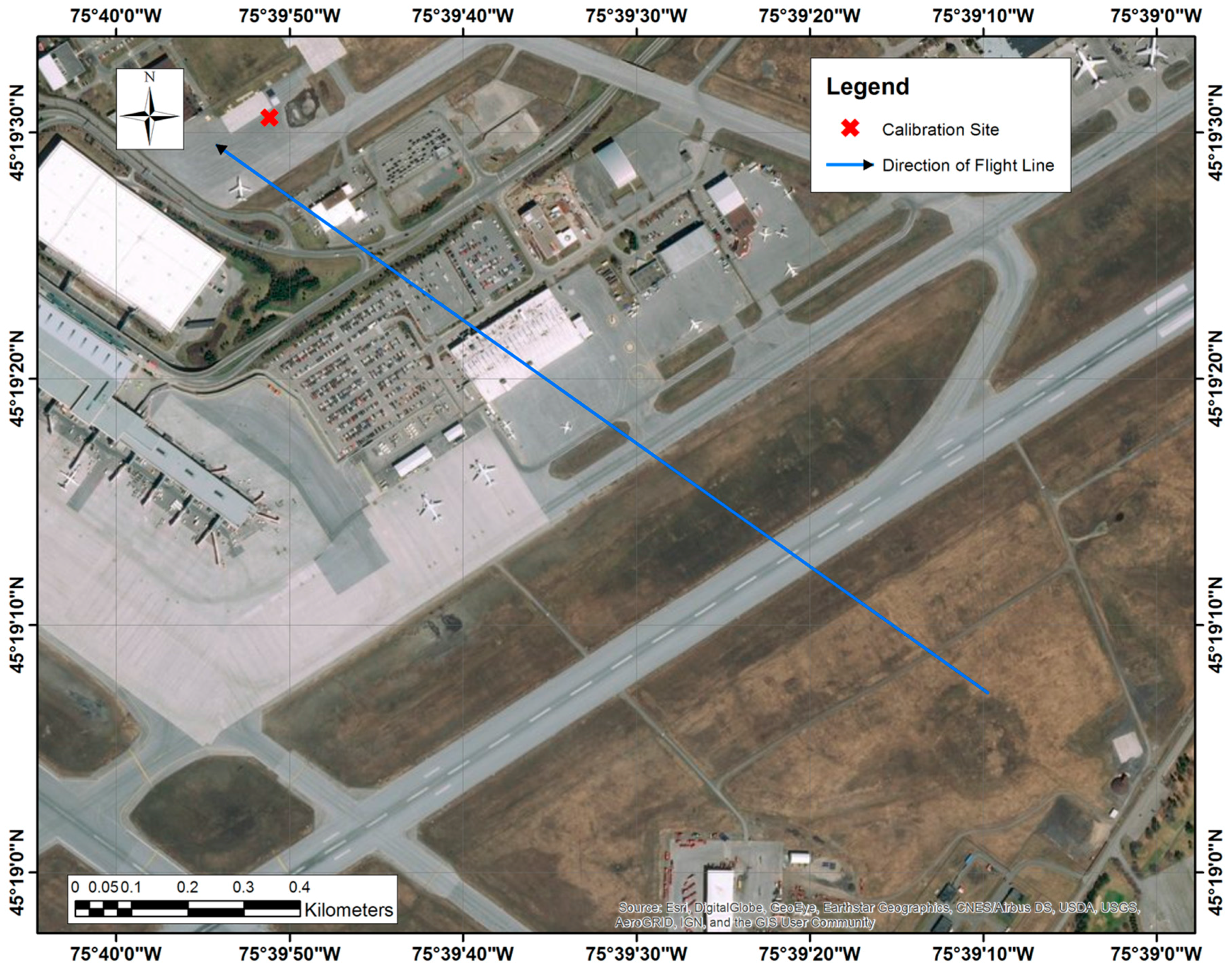
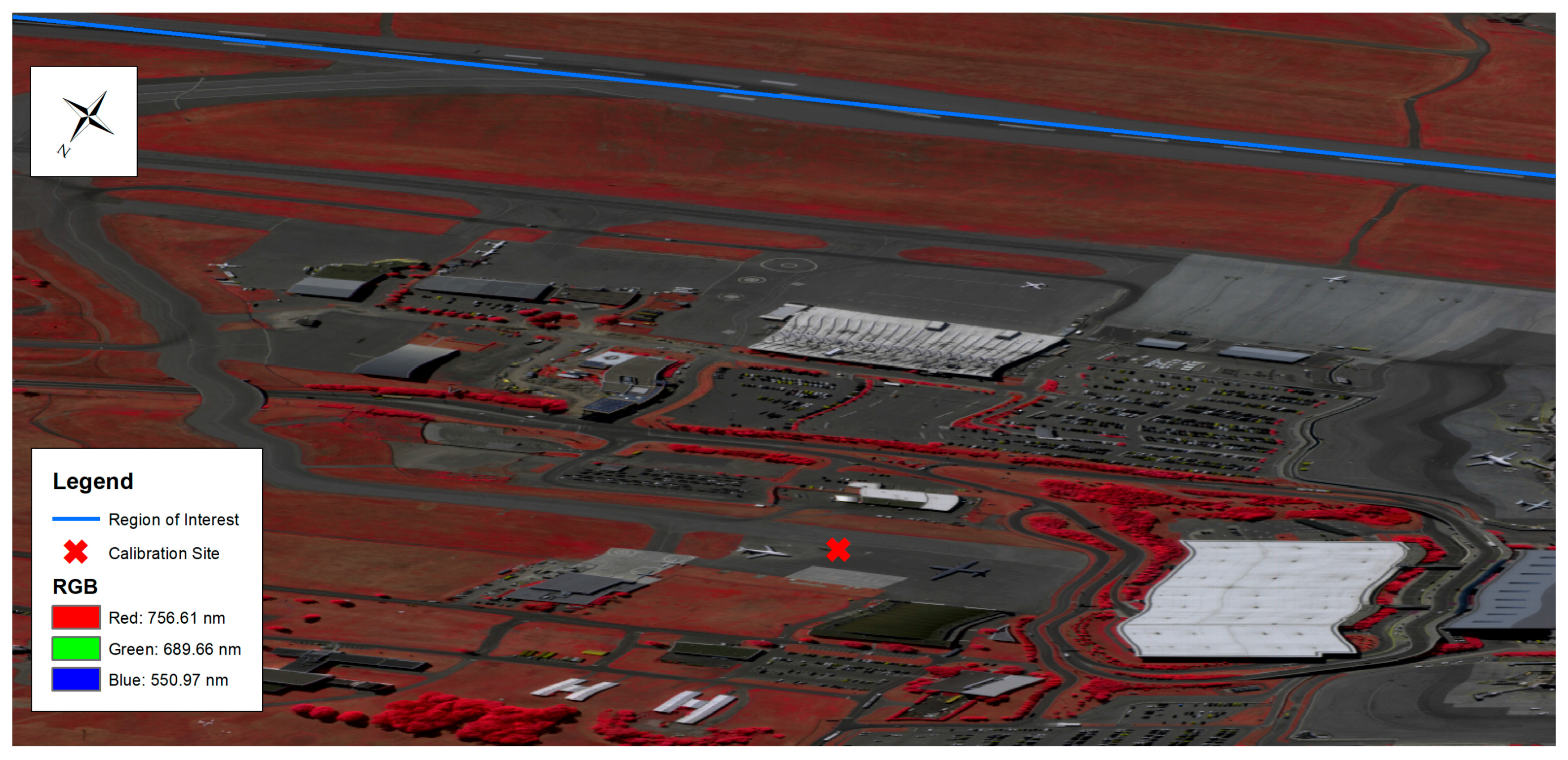
Airborne HSI data were acquired on 23 June 2016 at 14:53:13 GMT and 24 June 2016 at 13:24:16 GMT over the Macdonald–Cartier International Airport (containing the Flight Research Laboratory calibration site) in Ottawa, ON, Canada (Figure 2). Asphalt is an ideal target for real airborne acquisition as it is effectively ubiquitous in urban settings and can be found on the roadway systems surrounding the studied area. Furthermore, the surface reflectance of the material has a low amplitude (nearly flat), smoothly varying spectral response and is thus useful for in-field pseudo-calibration and validation [42].
Airborne imaging spectrometry data were acquired aboard the NRC’s Twin Otter fixed-wing aircraft with two complimentary HSI systems. The imagers each recorded an adjacent and partially-overlapping portion of the reflective electromagnetic spectrum between 366 nm and 2530 nm. Both imagers were manufactured by ITRES Research Limited. The first sensor system, the Compact Airborne Spectrographic Imager 1500 (CASI), acquired 288 bands (wavelength samples) within the 366–1053 nm range. The CASI is a variable frame rate, grating-based, pushbroom imager with a 39.7° FOV across 1500 spatial pixels. The device has a 0.49-mrad instantaneous FOV with a variable f-number aperture, configurable between 3.5 and 18.0. The second imaging system was the Shortwave Airborne Spectrographic Imager (SASI). The SASI is a prism-based pushbroom imager that acquires data from 160 spectral bands within the 885–2530 nm range with 640 spatial pixels across a 39.8° FOV. The device has an instantaneous FOV of 1.14 mrad and an aperture with a constant f-number of 1.8. Imagery is acquired at a fixed frame rate of 60 hertz with a programmable integration time of ≤16.6 ms. On both data acquisition days, imagery was obtained from a nominal height of 1115 m AGL with an approximate heading of 306.5° True North (Figure 2).
Prior to CC analysis, the HSI data underwent three pre-processing steps. The first step was a correction in the calibration to take into consideration the effects of small, but measurable pressure and temperature-induced shifts in the spatial-spectral sensor alignment. The second step was a spectroradiometric calibration that, following removal of estimated signal offset contributions (electronic offset, dark current, frame shift smear (CASI only), internal scattered light (CASI only) and 2nd order (CASI only)), converted the resulting radiance-induced digital pixel signal into units of spectral radiance (uW⋅cm−2·sr−1·nm−1). The final step was implemented to remove the laboratory-measured spectral smile by resampling the data from each spatial pixel to a uniform wavelength array. Although most of the spectral smile effects are removed by this pre-processing, extremely small residual effects may remain. Geocorrection of the data was not performed in order to preserve the original spectral response per pixel.
The described pre-processing methodologies utilized NIST traceable calibration data provided by the sensor manufacturer. Using the initial calibration data, various artefacts were identified in the resulting calibrated imagery. Independent of this study, the processing methodology was updated to refine the steps described above, resulting in new calibration programs and calibration data files. This refined processing removed many of the identified artefacts in the data. The CC analysis was performed on the raw imagery after being processed with both the initial and refined calibration files and methodologies. Overall, the study examined 8 datasets: the four raw hyperspectral images collected by the CASI and SASI over the two acquisition dates processed with both the original and refined processing methodologies.
2.3. Characterization of the Correlation Coefficient with Averaged and Interpolated In-Situ Radiance Hyperspectral Data
Before the CC was applied to the airborne imagery, the sensitivity of the statistical tool needed to be characterized with respect to the natural variances within asphalt spectra. This was accomplished by calculating the CC between each of 10 raw in-situ hyperspectral radiance measurements and their averaged spectral response.
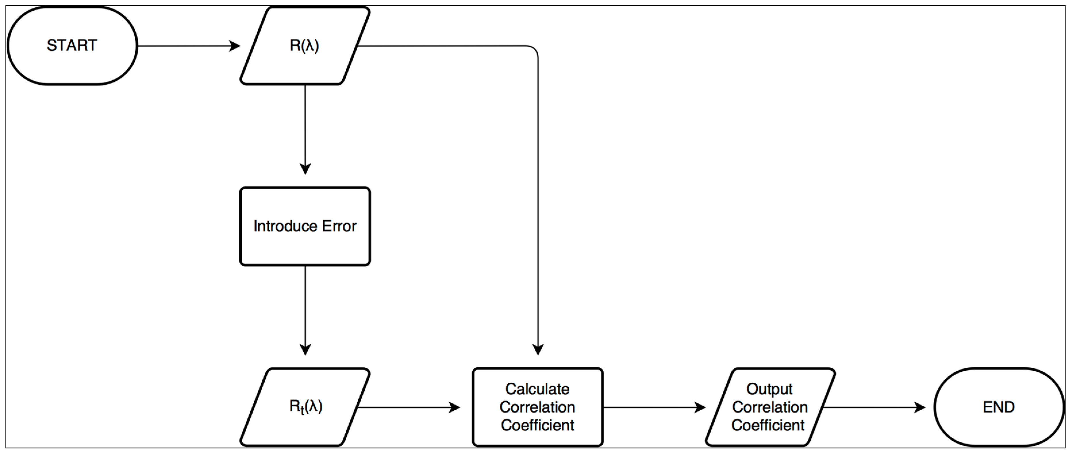
The sensitivity of the CC to common signal issues in HSI data was also characterized by artificially inducing errors in , the spectral response derived in Section 2.1. Five artificial errors were introduced independently by modifying in accordance with Table 1 to generate a variety of transformed signals, . The following modifications were applied: introduction of additive white Gaussian noise (AWGN), additive transformation, multiplicative transformation, introduction of spectral shift and multiplicative transformation of a single feature. The transformation models in Table 1 were developed to mediate the desired modifications. Parameters were carefully selected to mimic realistic potential errors. The AWGN modification was applied to generate a transformed spectral response with a specified signal-to-noise ratio, SNR. SNR designates the ratio between the energy of the original signal and the generated noise. For example, to obtain an SNR of 100:1, 4.31% AWGN was added to the signal. , and represent the additive factor, multiplicative factor and spectral shift (in nm), respectively, used to carry out each modification. Although there was no reason for the additive and multiplicative modifications to influence the CC, these tests were included to help provide a clear understanding of the approach. The multiplicative transformation of a single spectral feature was mediated through a normal distribution scaled by and vertically shifted with a minimum value of 1. and corresponded to the standard deviation and mean values, respectively, of the distribution. A normal distribution was used for the multiplicative factor to ensure the feature remained continuous along the edges of the spectral feature. was selected to capture the atmospheric absorption feature centered at 935 nm. The of 12 nm was chosen to ensure that the shoulders of the feature between 899 nm and 971 nm were within 3 of . α was varied from 1–50 to control the degree to which the absorption feature was modified.
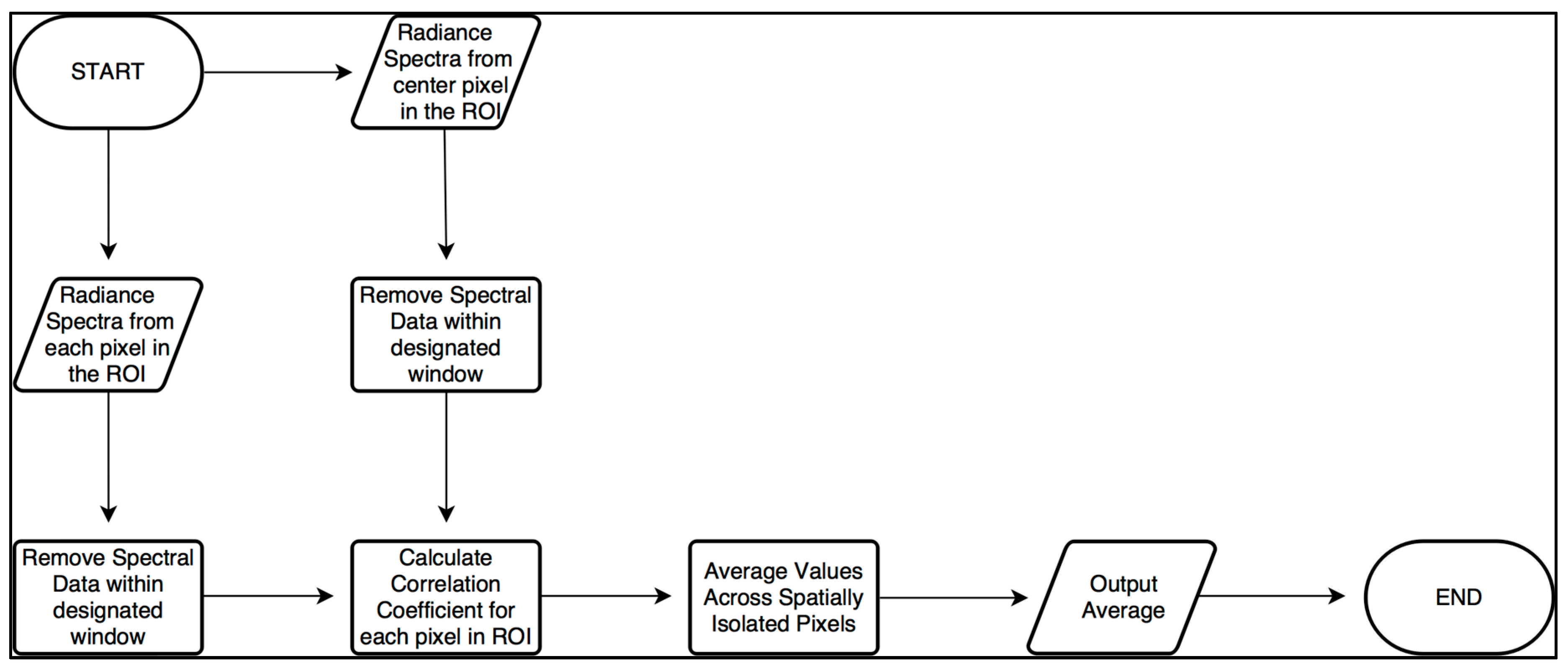
The tested ranges of values for SNR, , and were selected to introduce nominal to substantial errors. The CC was calculated between and each of the transformed datasets, , in accordance with Figure 3.
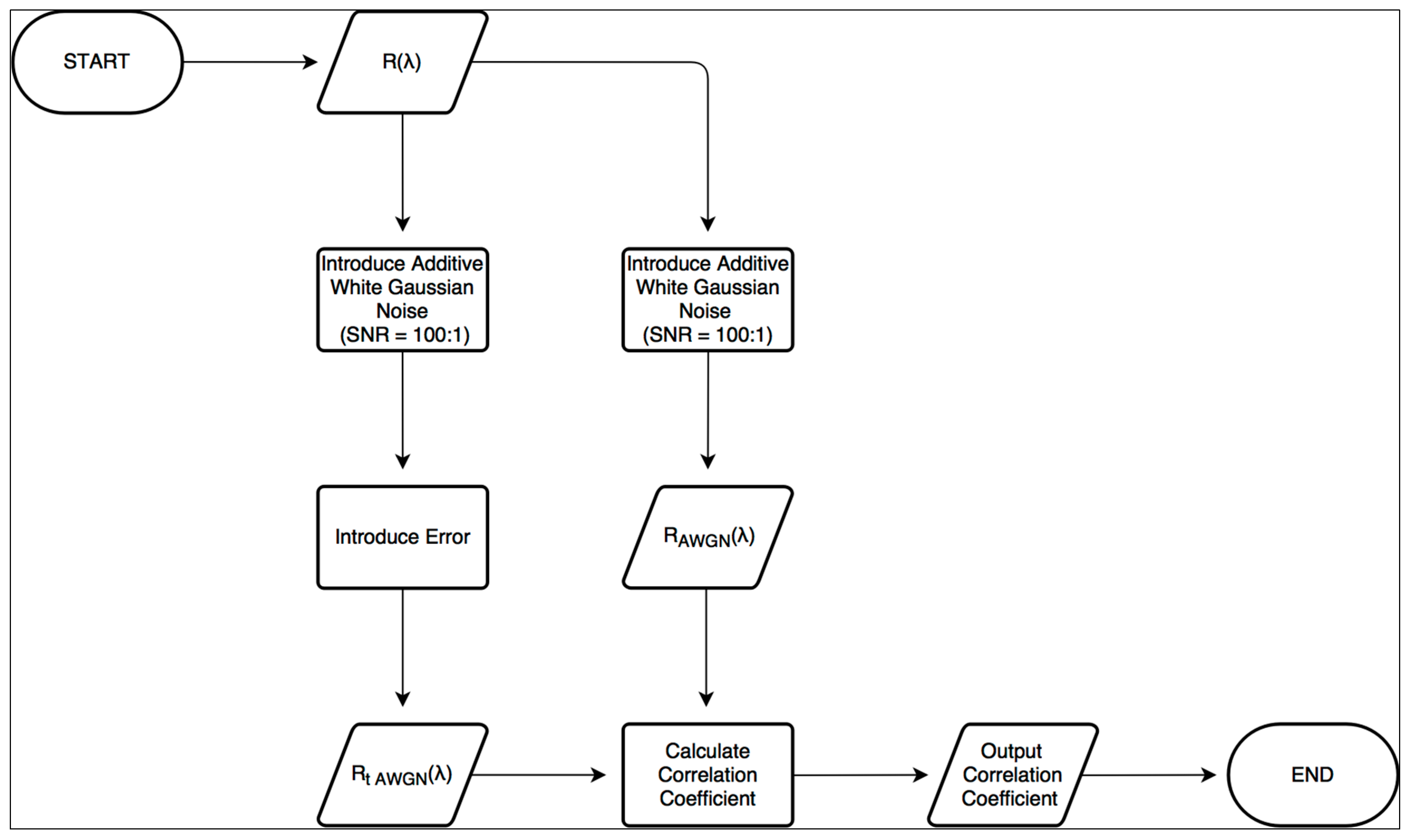
To test the persistence of the acquired trends with the presence of signal noise, the CC calculations for the last four modifications were repeated with AWGN. In particular, 4.31% AWGN was introduced to to acquire a new radiance signal, , with an SNR of 100:1, a reasonable value for airborne HSI data. A new transformed signal, , was acquired by applying transformation models from the last four rows of Table 1 to after introducing AWGN to generate a signal with an SNR of 100:1. The CC was calculated between and each in accordance with Figure 4.
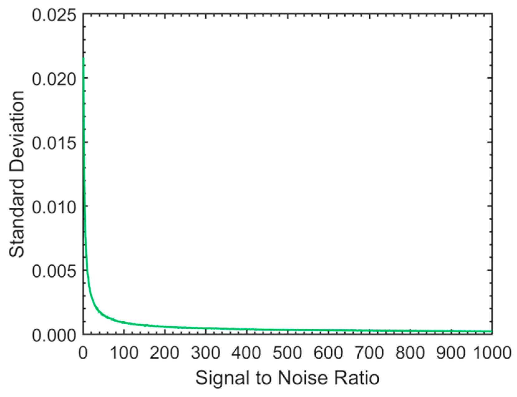
As a final test of consistency, the standard deviation of the CC was assessed in the presence of noise. In particular, the AWGN transformation in Table 1 was applied to 1000 times. A CC was calculated between and each of its transformations. The standard deviation of the CCs from each distinct SNR was calculated.
2.4. Application of the Correlation Coefficient to Airborne Hyperspectral Imagery (Error Detection)
Before applying the CC, a region of interest (ROI) (blue line in Figure 5) was identified across the FOV, along the taxiway located directly south of the calibration site. The ROI was comprised of a single asphalt road pixel from each column within the sensor FOV. Every attempt was made to acquire spectra from asphalt pixels that were uncontaminated by non-asphalt substances such as paint, vegetation and other non-asphalt hydrocarbons. “Wobbles” in the imagery in Figure 5 are caused by the movement of the aircraft and can be readily accounted for through various geocorrective methodologies. In this work, it was fundamental to preserve the original sensor geometry in the analysis, so no geocorrection process was applied.
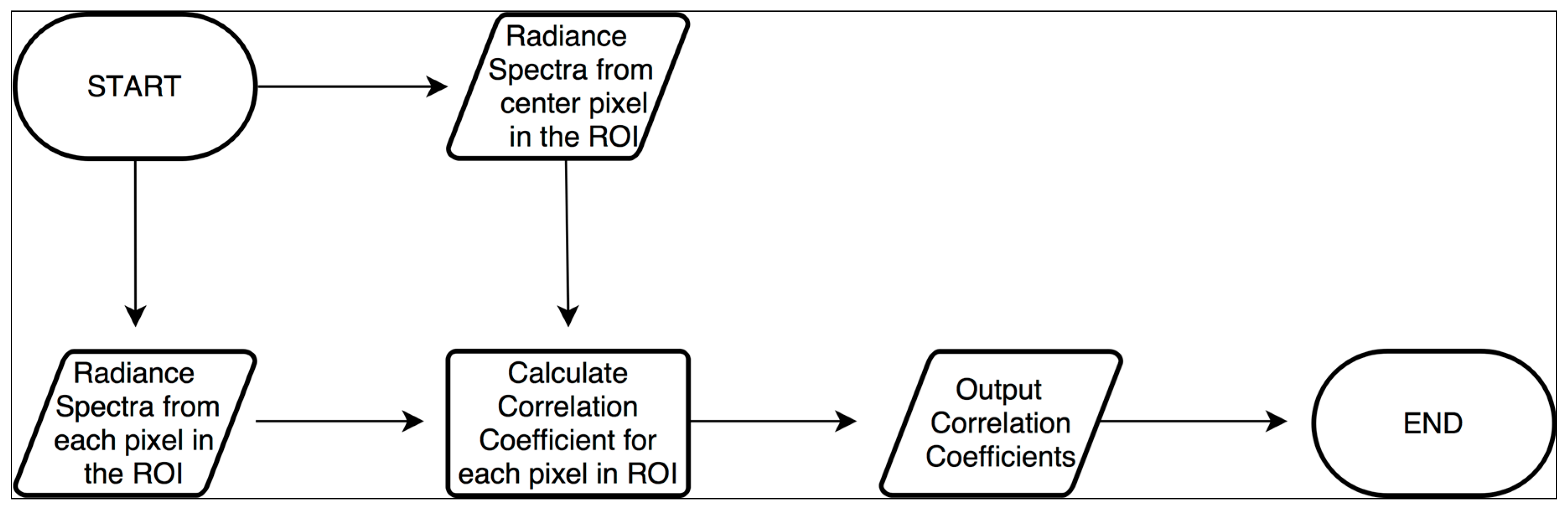
The spectrum from the center asphalt pixel in the ROI was designated as the reference for the application of the CC since it was the center of the instruments’ FOV. The center pixel was evaluated to ensure that it was a reasonable reference that contained no obvious errors. A CC was calculated between the spectrum from each pixel in the ROI and the designated central pixel reference in accordance with Figure 6.
Theoretically, the CCs should be exactly 1 across the FOV. Although this is not the case in real data, the CC between well-behaved target spectra will vary around a mean value that is still quite close to 1. The spatial pixels associated with substantial reductions in the CCs were recorded as potential locations for errors in the HSI data. Substantial reductions were characterized by CCs that fell below a designated threshold that was derived from the sensitivity testing.
To calculate the threshold, a stable spatial region was manually identified by consistent CCs that varied around a constant mean. Using the mean CC of this region, the SNR of a stable spectrum was approximated using the noise sensitivity data derived in Section 2.3. With the approximate SNR, the data from the final test in Section 2.3 were used to estimate the expected standard deviation of the CCs derived from stable spectra. Using the estimated standard deviation and the mean value of the CCs in the stable region, potential errors were detected by reductions more than below the mean. A threshold was selected to ensure that at least 99.7% of the stable data were not flagged as a potential error. Consequently, CCs below the threshold were likely associated with errors in the HSI data.
To spectrally isolate the potential errors in the recorded spatial locations, the CCs across the ROI were recalculated after removing the data in pre-defined spectral windows. The schematic in Figure 7 was carried out for various spectral windows. The spectral windows were designed to vary in size and spectral location. The window sizes were selected to ensure that windows contained anywhere from 1 to half of the total spectral bands. For any given size, the window was spectrally located beginning at the lower boundary of the spectral range. Each window was shifted by 5 nm until its edge surpassed the upper boundary of the dataset. For each window size and location, the average CC was calculated across the spatial regions associated with the detected potential errors. By maximizing the average CC over these regions, it was possible to identify the spectral window that was associated with a majority of the studied potential error.
To verify the spectral window and specify the nature of the potential errors, the imagery was visualized for a single band within the identified spectral ranges. In this visualization, image intensities were histogram equalized to enhance contrast by making the histogram of the resulting image equalized to a constant value. To verify that the reductions in the CCs were associated with these errors, the CCs were calculated across the FOV with respect to the center pixel after the removal of the identified spectral region.
Atmospheric absorption features were used to locate finer errors in the imagery that might not be easily visible in the CCs when calculated with the entire spectrum. These features were manually identified in the spectrum of the center asphalt pixel using the theoretical locations in Table 2 for guidance.
Atmospheric absorption features are distinctive and constant under stable conditions [45]. As such, the CC was thought to be able to detect inconsistencies in these regions since error-induced changes located within these features are more easily identifiable. As depicted in Figure 8, a CC was calculated between the spectrum from each pixel in the ROI and the designated central reference pixel using only the hyperspectral data that corresponded to each of the approximate wavelength regions identified in Table 2.
For each spectral range, the imagery was visualized for a single band within the specified window to study the nature of any detected errors. Once again, image intensities were histogram equalized to enhance contrast and clearly display potential errors. The methodologies presented in this section were repeated for each of the 8 processed images described in Section 2.2.
3. Results
3.1. In-Situ Ground Hyperspectral Data
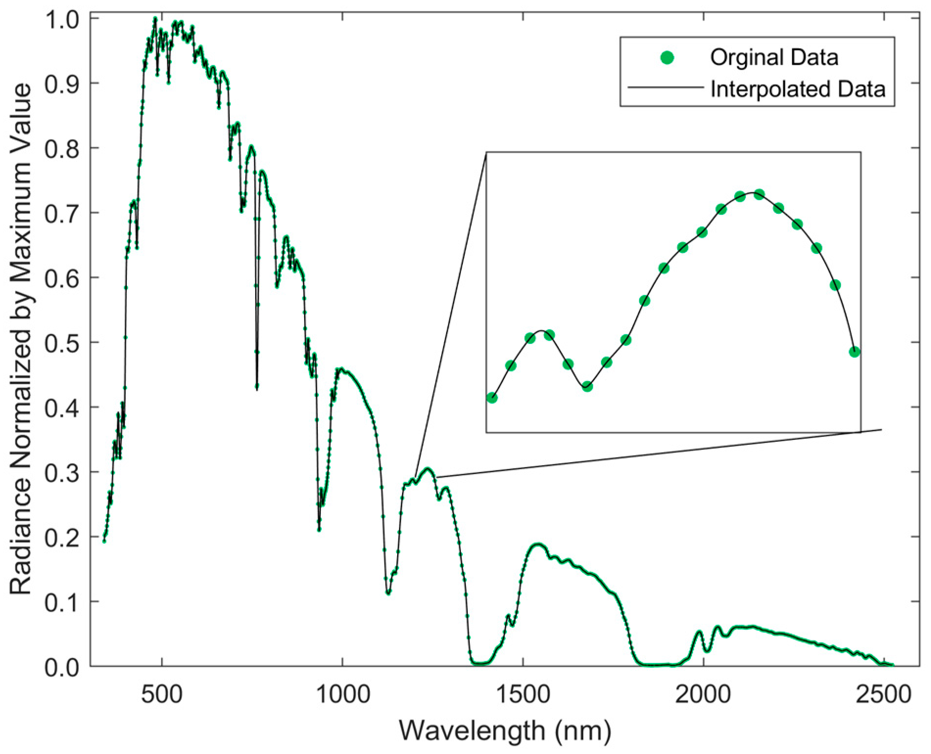
The data points in the normalized and averaged in-situ radiance signature were preserved after the Akima interpolation process was applied to generate (Figure 9).
.
3.2. Characterization of the Correlation Coefficient with Averaged and Interpolated In-Situ Radiance Hyperspectral Data
The CC between the mean in-situ asphalt radiance and any given individual sample used to comprise the mean signal was very close to one, ranging from 0.99987–0.99998, with a standard deviation of 0.000023.
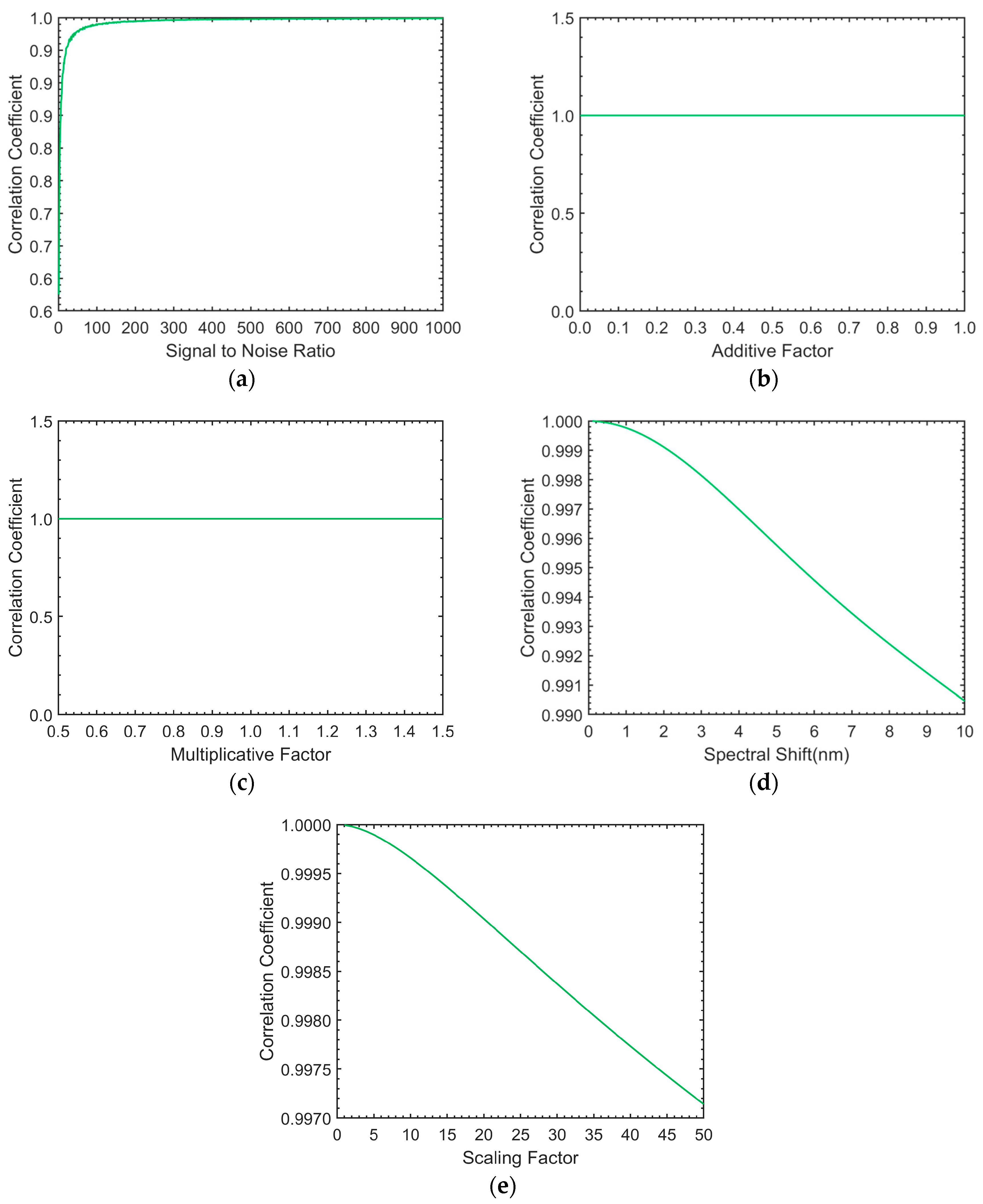
The CC decreased with the addition of AWGN (Figure 10a). At SNR values below 9:1, the CC was under 0.9. As the SNR increased, the CC raised in an asymptotic fashion. After reaching an SNR of 1000:1, the CC equilibrated at approximately one. The CC remained constant at one for all linear transformations (Figure 10b,c). As the spectral shift increased from 0–10 nm, the CC decayed from a value of 1–0.991 (Figure 10d). A similar result was found after the atmospheric absorption feature at 935 nm was modified. In this case, the CC reduced from one to a value of 0.9970 as the scaling factor increased (Figure 10e).
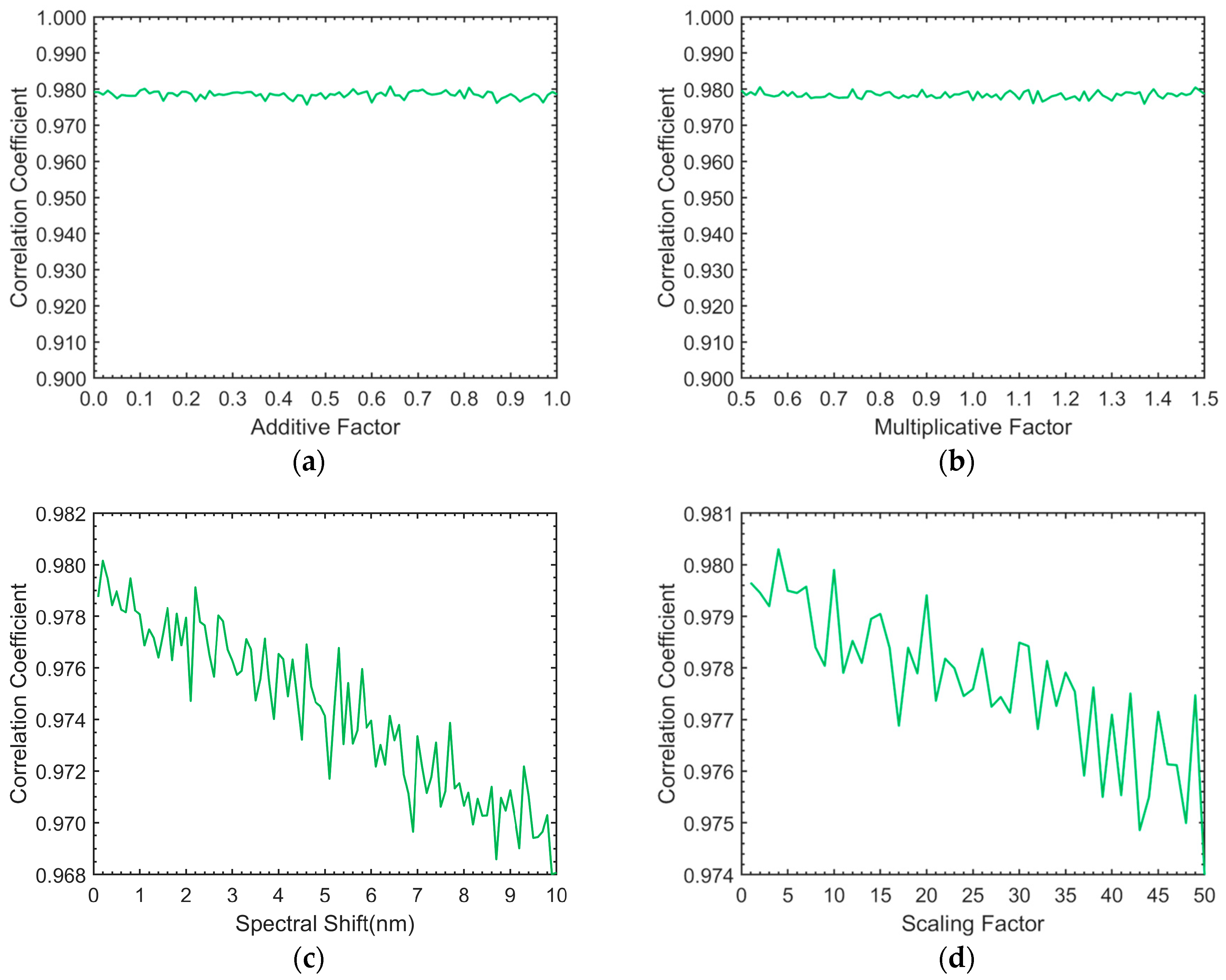
As can be seen in Figure 11, the general trends outlined in Figure 10b,e persisted even after the application of AWGN at an SNR of 100:1.
The CC remained invariant to linear transformations (Figure 11a,b). However, the average value of the CC reduced to approximately 0.98. Although the detailed relationships in Figure 11c,d were masked by the variation induced by the introduced noise, the first-order trends are clearly present and identifiable. The CC reduced from 0.980–0.968 after a 10 nm spectral shift in Figure 11c. As the scaling factor increased from 0–50, the CC decreased from 0.9815–0.975. At an SNR of 100:1, the average standard deviation in the CC for each modification was approximately 0.001. As seen in Figure 12, this value matched the results derived from the final CC test, which calculated the standard deviation in the calculated CC at various noise levels.
At a SNR of 100, the standard deviation is approximately 0.001. The standard deviation in the CC asymptotically increased from zero to approximately 0.22 when the SNR decreased through the introduction of AWGN.
3.3. Application of the Correlation Coefficient to Airborne Hyperspectral Imagery (Error Detection)
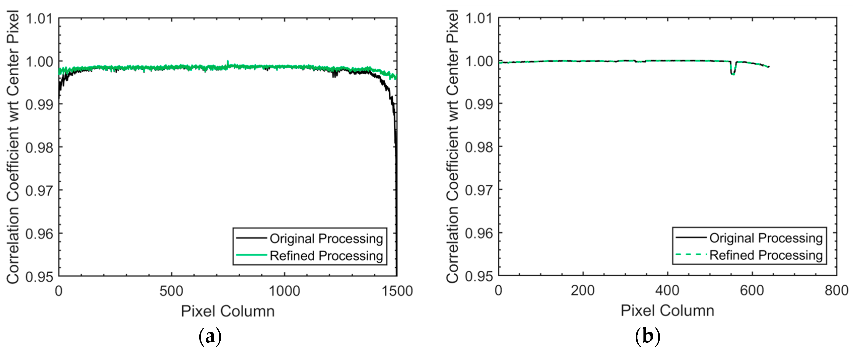
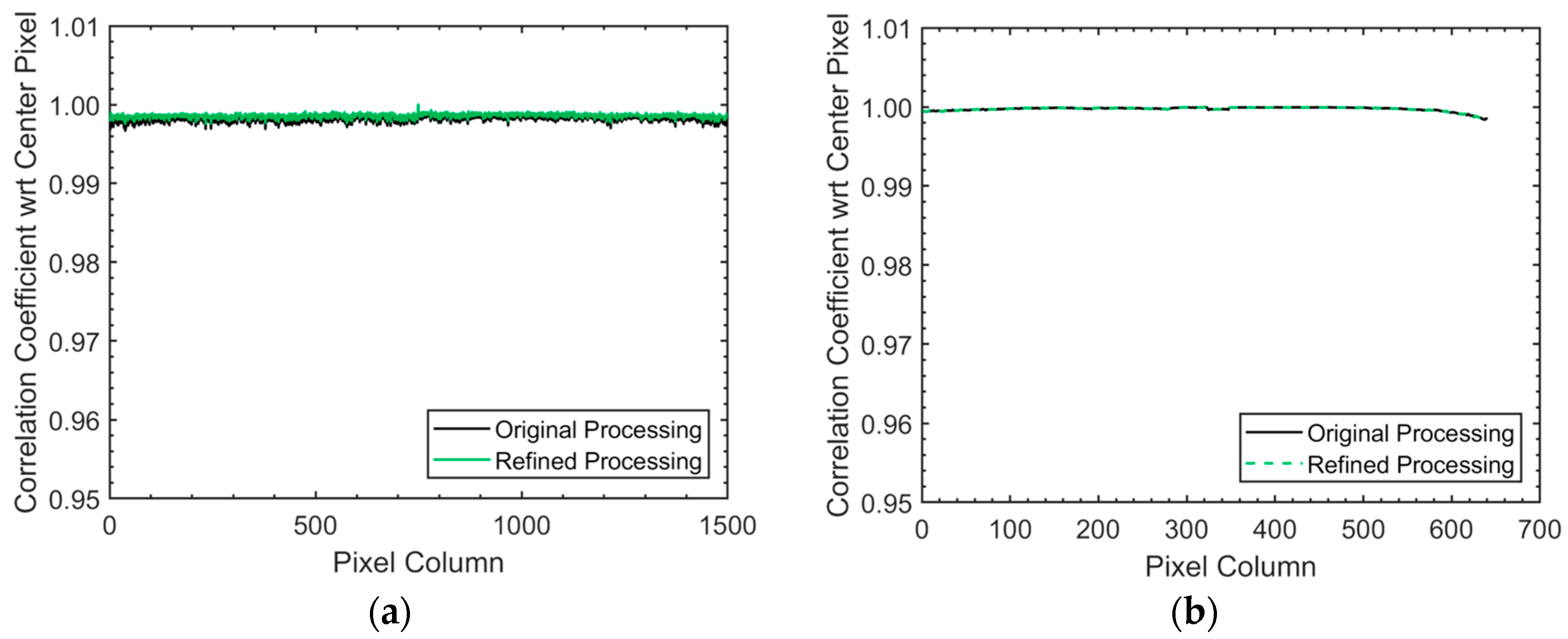
For each hyperspectral image, the calculated CCs recorded in Figure 13 adhered very closely to one across the FOV when calculated with respect to the spectrum from the center pixel. The CCs for the CASI imagery were consistently lower than that of the SASI by an average value of 0.0021 (Figure 13). In addition, the average standard deviation in the CCs of the CASI data was over 18-times larger than that of the SASI.
For the CASI imagery, the CCs systematically reduced in value by more than one standard deviation near the edges of the FOV. This reduction was largest for the CASI data derived from the original processing methodology. When compared to the imagery collected on the 23rd, the CASI data from the 24th were characterized by more substantial reductions in the CCs near the edges of the FOV, especially along the left side. The CCs for the SASI imagery were almost identical, regardless of the processing methodology or the acquisition date. The CCs for the SASI imagery were consistently lower than the mean across the FOV from Pixels 548–564. As seen in Figure 13b,d, this reduction appeared to be parabolic in nature, reaching a minimum value of approximately 0.995 and 0.997 in the SASI imagery from the 23rd and 24th, respectively.
The spatial locations associated with distinct reductions in the CCs were identified using the threshold defined in Section 2.4. These locations were used to spectrally isolate the potential errors to the windows identified in Table 3 using the windowed-based methodology described in Section 2.4.
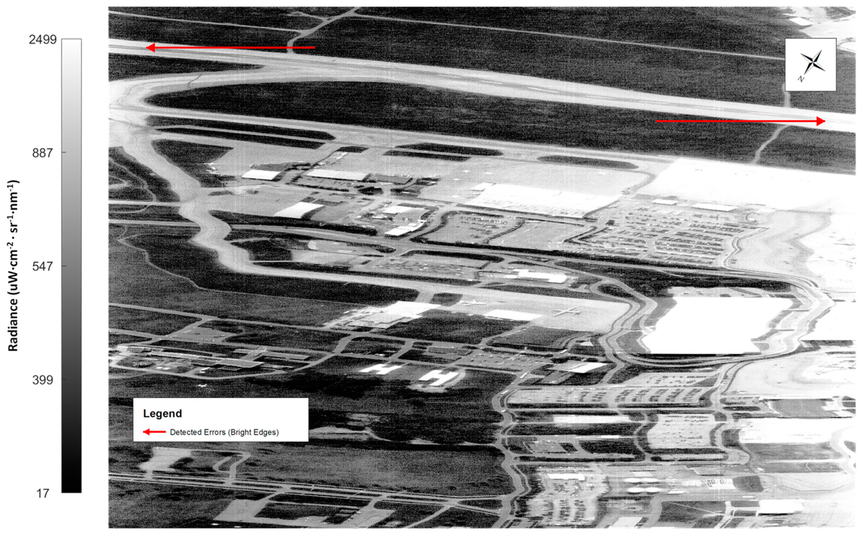
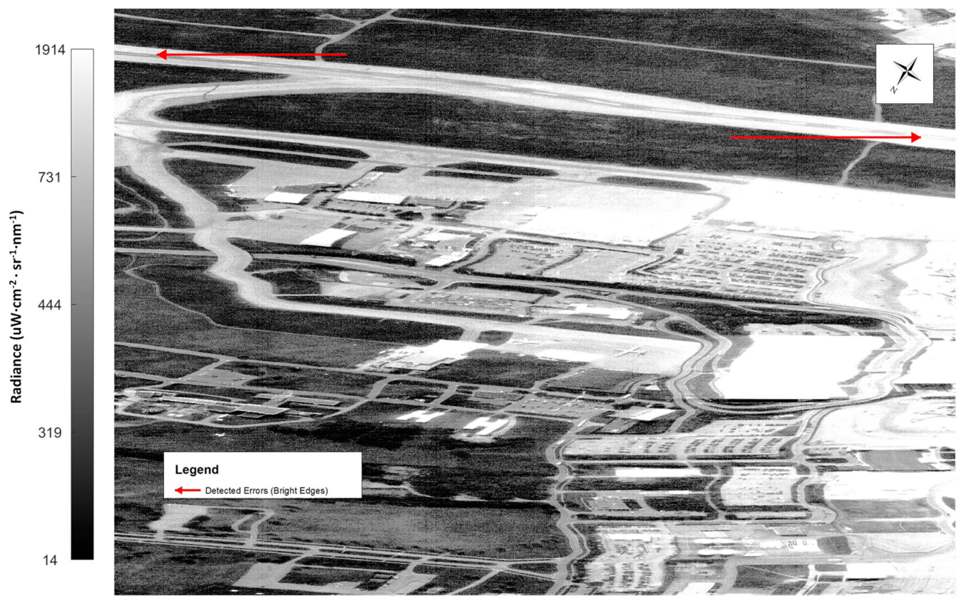
Errors in the imagery were clearly detected though the visualization of the spectral windows in Table 3. An example of the error in the CASI imagery is displayed in Figure 14. In the imagery, the asphalt road is clearly brightest along the edge pixels.
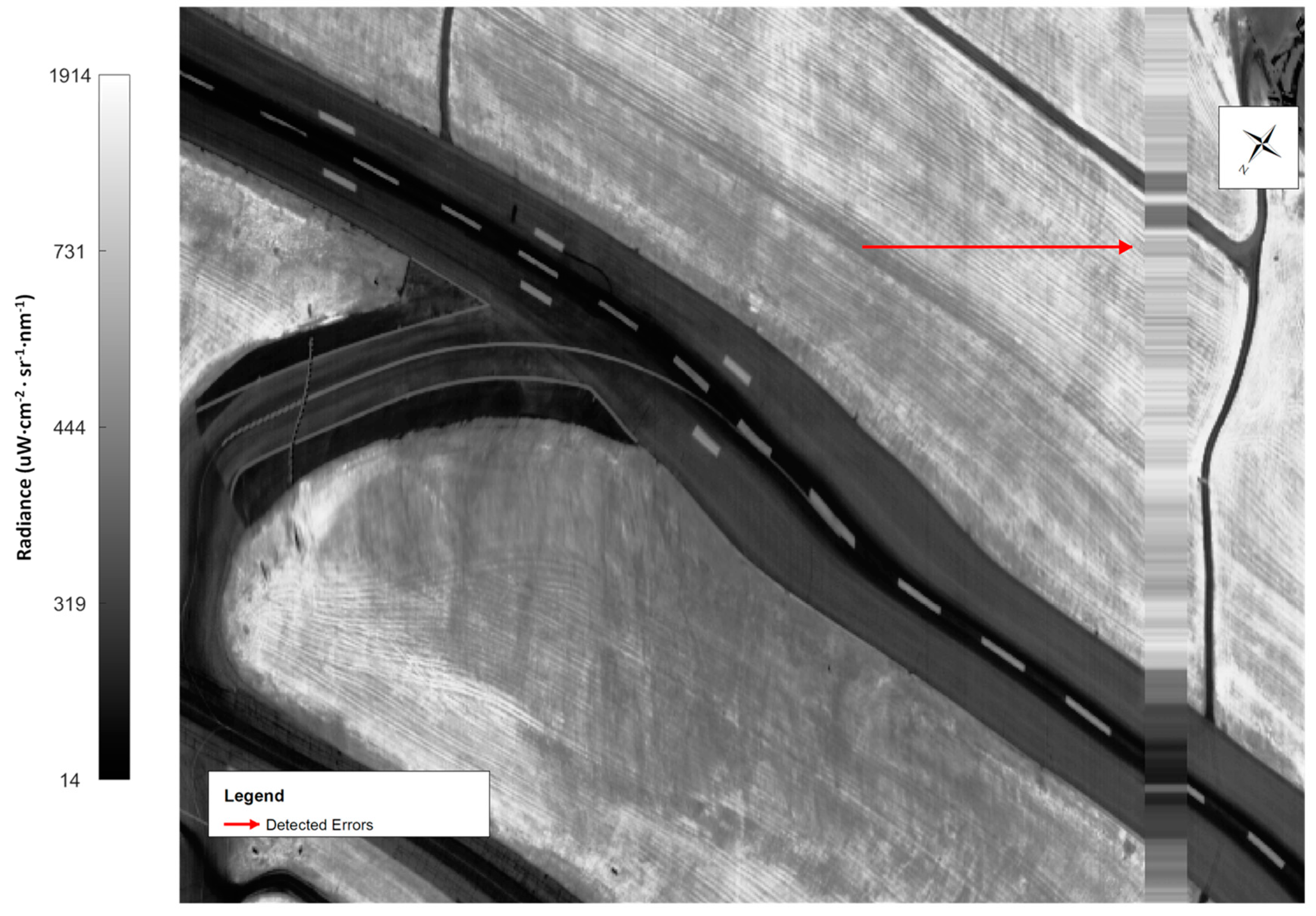
This general trend held for all CASI imagery and was less prominent with the refined processing methodology (Figure 15). The asphalt road is still brightest along the edge pixels, but to a lesser degree than in Figure 14.
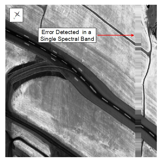
The error within all SASI imagery was located at the same spatial pixels and spectral range. The error could be displayed by visualizing the only band in the 993–1008 spectral range (Figure 16).
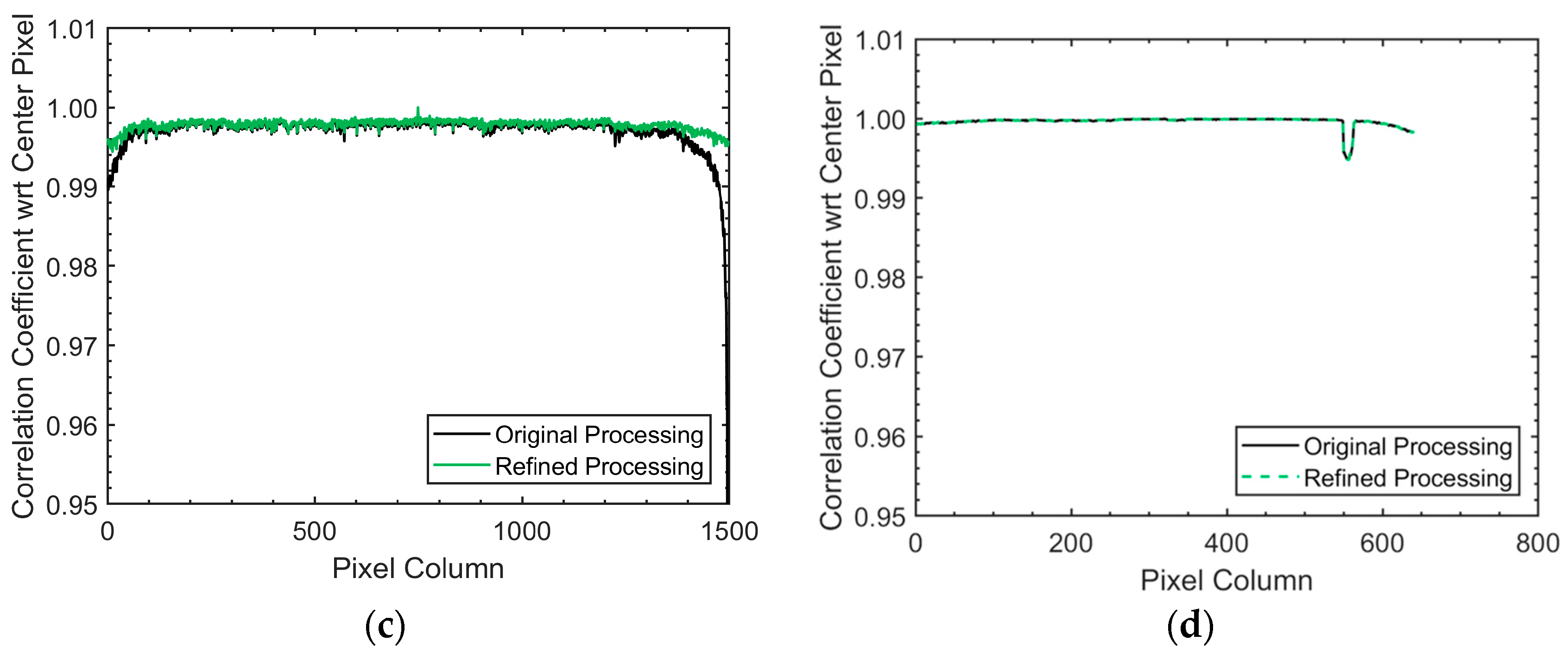
After removing data in the spectral windows in accordance with Table 3, there was a substantial increase in the values of CCs across the FOV in all images (Figure 17), especially at spatial locations associated with the previously identified imaging errors. Comparing Figure 13b,d and Figure 17b,d, the large reduction in the SASI imagery from Pixels 548–564 was completely removed. Furthermore, the CCs along the FOV of the CASI images remained relatively constant, even at the edge pixels. Overall, there was more consistency between the images derived by the different processing methodologies and acquisition dates.
Comparing Figure 13a,c to Figure 17a,c, there was more consistency in the CCs of the CASI imagery from the 23rd between the original and refined processing. Although this trend holds for the CASI data from the 24th, there was still a notable average offset of 0.0007 between the two curves. Significance testing yielded p-values less than 10−5 for all observed relationships.
To further the analysis and spectrally locate smaller residual errors in the CASI data from the 24th, five atmospheric absorption features were identified in the spectral range from 365–1050 nm (Table 4).
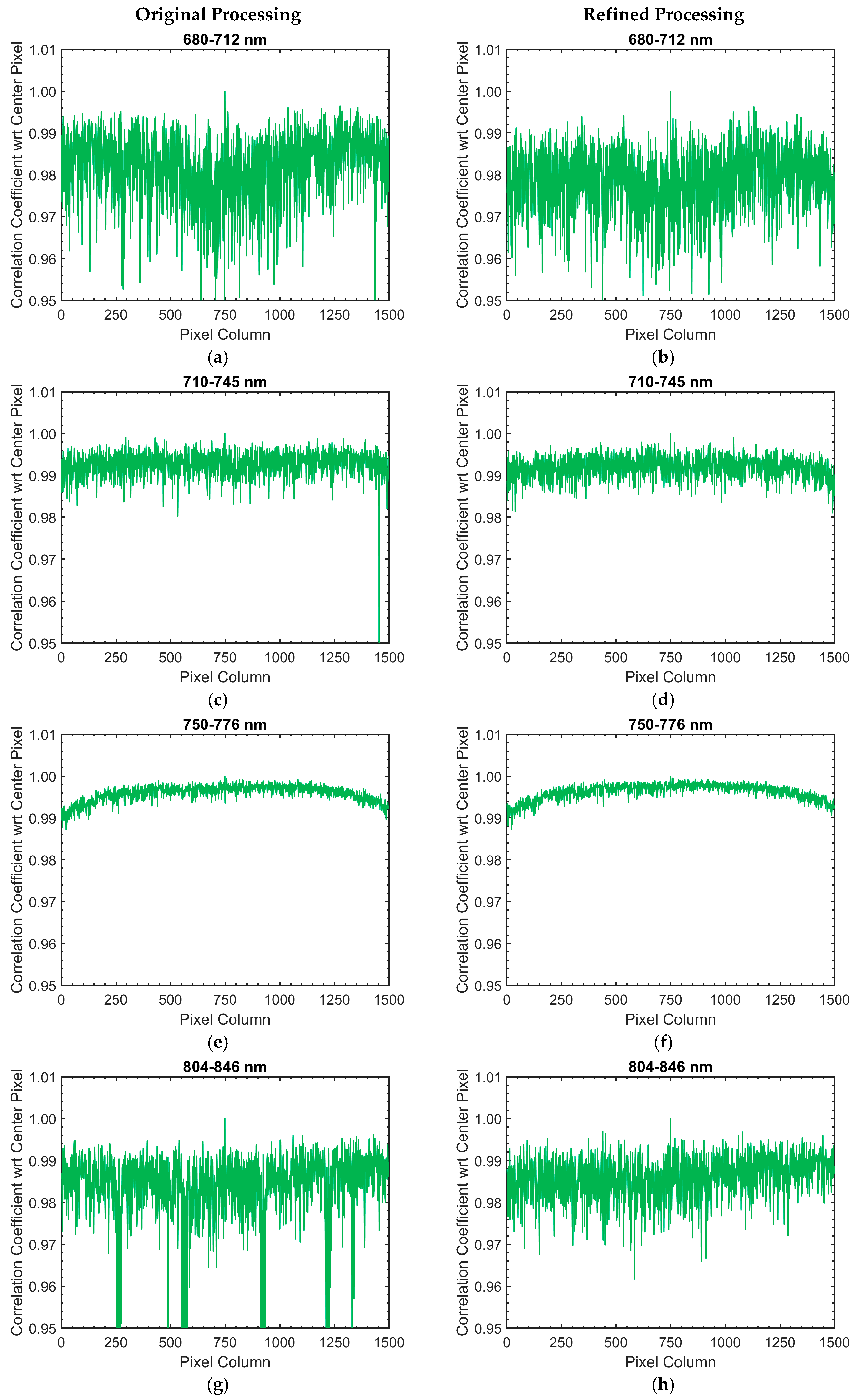
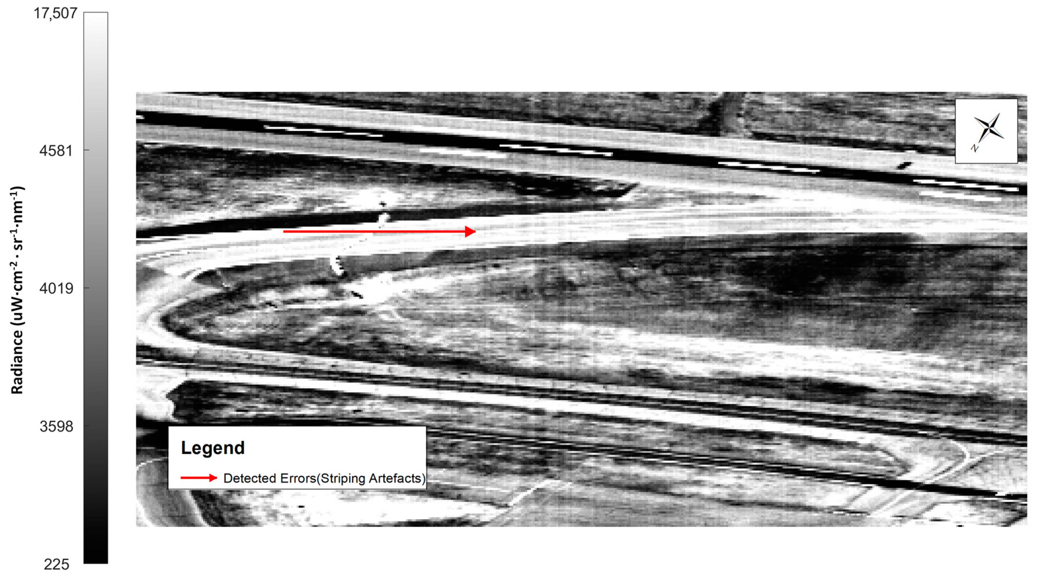
The CCs across the FOV of the CASI images from the 24th were calculated with respect to the center pixel over the spectral regions identified in Table 4 and are shown in Figure 18. The CCs in the 680–712 nm region were highly variable, ranging from 0.95–1 with a subtle low frequency sinusoidal structure (Figure 18a,b). Visual inspection of the associated imagery in Figure 19 indicated that, throughout much of the FOV, there were discrete pixels and groups of pixels that appeared to be non-uniform across the entire FOV, noticeably varying in brightness even amongst neighboring pixels. These pixels lead to “striping” artefacts across the entire FOV in the image data. These trends were apparent in both CASI images. The low frequency sinusoidal structure could not be clearly visualized in the imagery. The sinusoidal structure was not a numerical computational effect.
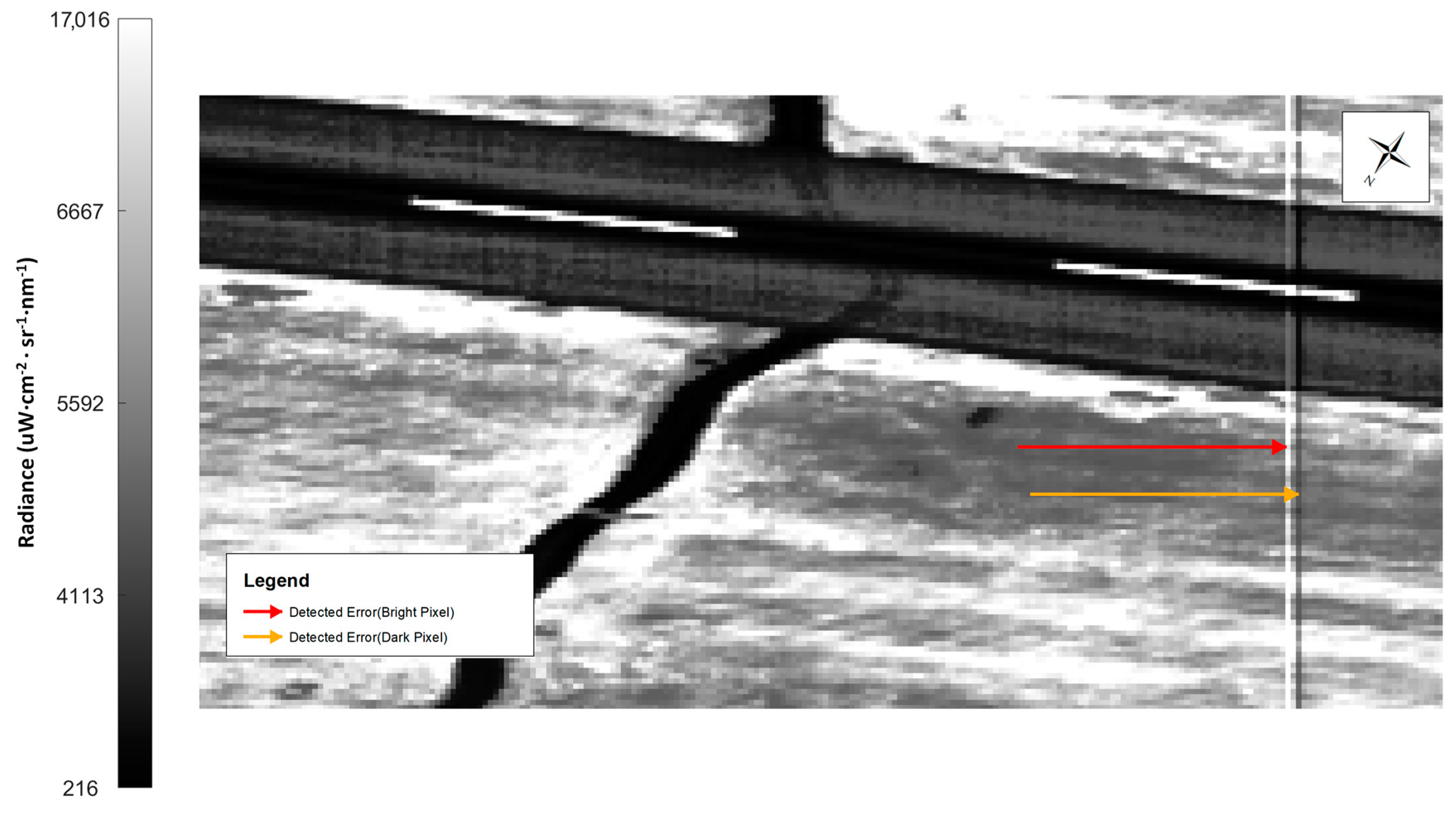
Although Figure 18c remained relatively consistent across the asphalt road, there was a sudden reduction near the end of the FOV at Pixels 1454 and 1456. After independently displaying all bands in the specified spectral window in greyscale, errors were spatially located in Columns 1454 and 1456; these errors were visualized as a bright and dark vertical stripe, respectively, across the imagery (Figure 20). The vertical stripes were not present in the CASI imagery with the refined processing or Figure 18d.
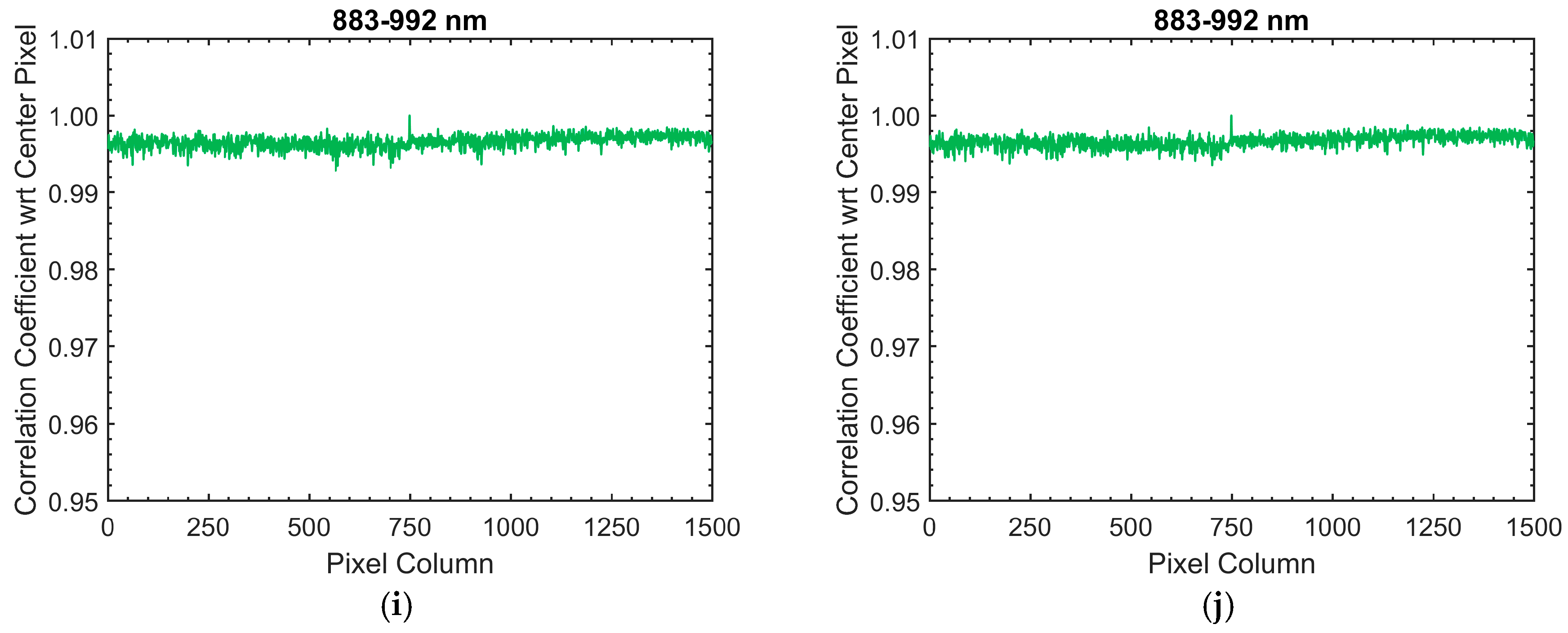
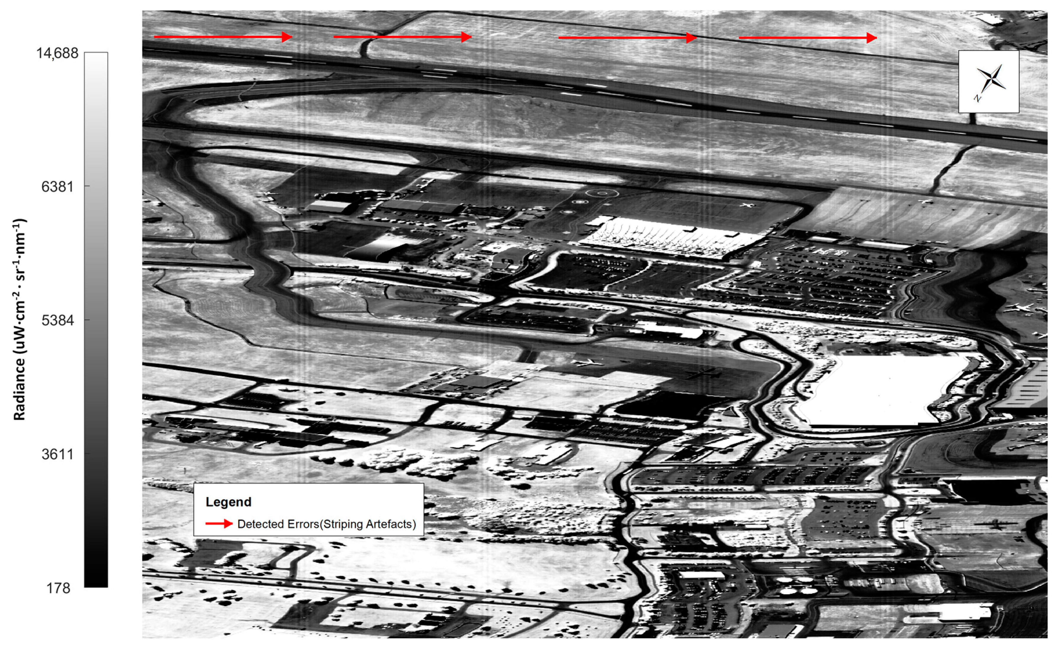
There was a reduction of approximately 0.021 in the CC near the edges of the FOV in Figure 18e,f. The effects associated with these reductions could not be visualized within the imagery. Figure 18g was characterized by sporadic reductions in the CC of greater than 0.05. These reductions revealed potential imaging errors for the spectral window in the following spatial ranges: 256–276, 551–576, 912–936 and 1209–1235. After independently displaying all of the bands in the specified spectral window in greyscale, it was possible to detect groups of non-uniform pixels that noticeably varied in brightness. These groups created distinct “striping” artifacts that can be seen at several spatially-isolated points across the CASI imagery from the 24th with the original processing (Figure 21). This effect was not present in the CASI imagery with the refined processing or Figure 18h.
4. Discussion
By characterizing the sensitivity of the CC before its application to real airborne HSI data, it was possible to verify the detective capabilities of the metric in the localization of errors in hyperspectral data. The findings generally agreed with all basic intuition and theoretical expectation of the CC. Linear transformations, in agreement with theory, had no impacts on the value of the CC. By calculating the CC between two similar spectra, the value could be used to gauge the consistency independent of the effects associated with linear transformations. Because of this property, the CC was shown to be extremely insensitive to the natural variances between different asphalt spectra. This was important for the detection of errors in HSI data as it implied that the differences in the calculated CCs were not primarily due to the variations between asphalt samples. All modifications, aside from the linear transformations, resulted in a consistent reduction in the CC. Consequently, the CC could detect spectral shifts and modified spectral features. Although the CC was sensitive to signal noise, all general trends held irrespective of the AWGN in hyperspectral data with an SNR of 100:1, which is a reasonably high noise level for airborne HSI data. This trend was fundamental to the application of the CC as it meant that the metric was sufficiently resistant to noise for the purposes of error detection; so long as errors are not being completely masked by noise, the CC can detect their presence. Implementing this knowledge, the CC was applied to real airborne HSI data.
Through the application of the CC, the quality of remotely-sensed hyperspectral data could be assessed through error detection in a quantitative manner. This was evident in the analysis of the eight hyperspectral images that were studied. By calculating the CCs across the FOV with the entire spectra, it was possible to immediately gauge the spectral consistency of the HSI data collected by the CASI and SASI, across the FOV. It is important to note that the method was explicitly designed for the detection of errors, not for the identification of their origin.
In the CASI imagery, the methodology was able to spatially detect errors along the edges of Figure 13a,c by systematic reductions in the CCs near the boundaries of the FOV. The spectral locations of these effects were found in the blue end of the spectrum, in accordance with Table 3. Visualization of the imagery in Figure 14 and Figure 15 revealed an error that is consistent with the effects of the spectral smile or other cross-track illumination effects [46]. With a greater decline in the CCs near the edges of the FOV, this error was more prominent in the CASI data collected with the original processing methodology. As such, it is possible to deduce that the refined processing was able to better correct for the effects observed at the edges. The CASI imagery from the 24th was characterized by slightly lower and more variable CCs then the data from the 23rd, especially near the edges of the FOV. With this information, there is some innate variability in the data acquisition of the CASI that could be quantified from the CCs.
The CCs of the SASI imagery were virtually identical regardless of the processing methodology and acquisition date. This suggested that the SASI was very stable in its data acquisition. Furthermore, it was clear that the refined processing methodology did not have a large impact on the data. Using the developed algorithms, an error was detected in the SASI imagery at a single spectral band by a reduction in the CCs from Pixels 548–564. This showcased the developed CC-based methodology as a strong tool in the localization of errors in imaging spectrometers.
After removing the data within the spectral windows identified in Table 3, there was a greater degree of consistency amongst all of the CASI and SASI images. That being said, not all datasets perfectly aligned; there was a slight offset between the CASI images collected from the 24th. To investigate the discrepancy in the CASI images from the 24th, finer errors were detected in the regions that surrounded the five atmospheric absorption features in Table 4. All but one of the spectral regions was characterized by non-uniform CCs across the FOV (Figure 18). The irregular structure in Figure 18a,b was caused by non-uniform pixels, which noticeably varied in brightness. This error created “striping” artefacts across the image data. These artefacts have been observed in the literature and are likely due to radiometric calibration errors [47]. Although the origin of the low frequency sinusoidal structure could not be established, it is clear that the trend is not a numerical computational effect. As such, there is likely a subtle wide spatial scale feature. The origin of the subtle feature in the CCs is still being investigated. The sporadic reduction in the CCs of Figure 18c detected errors at Pixel Columns 1454 and 1456, which were visualized as a bright and dark vertical stripe, respectively, across the imagery (Figure 20). Since this reduction was not present in Figure 18d, the refined processing methodology was able to correct for this error. Based on the structure of the CCs near the edges of the FOV in Figure 18e,f, there were potential residual smile effects or other cross-track illumination effects that could not be clearly visualized in the imagery. The sporadic reductions in the CC of Figure 18g revealed groups of non-uniform pixels that created distinct “striping” artefacts that can be seen at several points across the CASI imagery from the 24th with the original processing (Figure 21). These errors were not present in Figure 18h or its associated imagery. As such, the refined processing methodology was able to correct for this error. The relatively constant CCs across the FOV in Figure 18i,j corresponded with stable imagery within the designated spectral window, as displayed in Figure 22. This information is fundamental as it showcases that the CC method can detect stable imagery, when it is present. The offset between the CASI imagery collected on the 24th in Figure 17 was likely due to the additional errors that were not corrected in the original processing methodology.
Although significance testing yielded p-values less than 10−5 for all observed relationships, it is important to note that these values did not necessarily imply practical significance. This was due to an issue inherent to the p-value itself; with such a large sample size and small variance, significance testing flagged even the most subtle of changes as significantly different [48]. Fortunately, this was not an issue within the study as all of the flagged potential errors could be visualized and verified in the imagery itself. A similar statement can be made for the differences observed in the CCs between the distinct processing methodologies and acquisition devices.
Overall, errors were detected in the CASI and SASI imagery though the application of the CC. Although more sophisticated error detection methodologies exist (e.g., [37,39,40]), they can be monetarily expensive to implement and rely on a higher level of mathematical understanding. Without a fundamental understanding of a method, its implementation can lead to inaccurate interpretations. The presented method is intuitive; the CC is a rather simple statistical tool and its application is straight forward. The detection can be conducted on radiance spectra prior to atmospheric correction, quickly after acquisition. After removing the wavelength region associated with large errors, the described methodologies could be repeated to isolate smaller errors. Although the application was developed for hyperspectral technologies, it can be easily generalized for data collected by other imaging spectrometers. This versatility showcases the CC as a strong and simple statistical tool for the analysis of spectrographic imaging data through the detection of errors.
5. Conclusions
This work substantiated the versatility of the CC with respect to the localization of errors in spectrographic imaging data. The sensitivity of the CC was characterized with respect to subtle spectral changes in the averaged in-situ level radiance data. Errors were spectrally and spatially detected in real airborne acquired HSI data. As per the original intent of the study, the methodology was successfully developed for the detection of errors, not for the identification of their origin. The method was able to gauge the effectiveness of various processing methodologies and the imaging systems themselves. Overall, the CC is clearly a strong, simple, low monetary cost, analytical tool for studying hyperspectral remotely-sensed data quality through error detection.
Acknowledgments
This work was funded by the Flight Research Laboratory of the National Research Council of Canada, the National Sciences and Engineering Research Council of Canada and the Rathlyn Fellowship. The authors would like to thank Gabriela Ifmov, Thomas Naprestek, Daniel Macdonald and Shahrukh Alavi for supporting data acquisition; and Anthony Brown, Derek Gowanlock and Paul Kissman for piloting the Twin Otter. The authors also thank the two anonymous reviewers, whose comments helped to improve this manuscript. The authors would like to express their appreciation to Defence Research and Development Canada Valcartier for the loan of the CASI instrument.
Author Contributions
G.L. conceived of the study. G.L. and D.I. developed the algorithms. R.J.S., D.I. and G.L. collected the data. D.I. processed the data. D.I. and G.L. analyzed the data with input from R.J.S. and M.K. D.I. wrote the manuscript with input from G.L., M.K. and R.J.S. G.L., M.K. and R.J.S. edited the manuscript.
Conflicts of Interest
The authors declare no conflict of interest. The founding sponsors had no role in the design of the study; in the collection, analyses or interpretation of data; in the writing of the manuscript; nor in the decision to publish the results.
References
- Green, R.O.; Eastwood, M.L.; Sarture, C.M.; Chrien, T.G.; Aronsson, M.; Chippendale, B.J.; Faust, J.A.; Pavri, B.E.; Chovit, C.J.; Solis, M. Imaging spectroscopy and the airborne visible/infrared imaging spectrometer (AVIRIS). Remote Sens. Environ. 1998, 65, 227–248. [Google Scholar] [CrossRef]
- Cloutis, E.A. Review article hyperspectral geological remote sensing: Evaluation of analytical techniques. Int. J. Remote Sens. 1996, 17, 2215–2242. [Google Scholar] [CrossRef]
- Van der Meer, F.D.; van der Werff, H.M.A.; van Ruitenbeek, F.J.A.; Hecker, C.A.; Bakker, W.H.; Noomen, M.F.; van der Meijde, M.; Carranza, E.J.M.; Smeth, J.B.D.; Woldai, T. Multi- and hyperspectral geologic remote sensing: A review. Int. J. Appl. Earth Obs. Geoinf. 2012, 14, 112–128. [Google Scholar] [CrossRef]
- Murphy, R.J.; Monteiro, S.T.; Schneider, S. Evaluating classification techniques for mapping vertical geology using field-based hyperspectral sensors. IEEE Trans. Geosci. Remote Sens. 2012, 50, 3066–3080. [Google Scholar] [CrossRef]
- Xu, H.; Wang, X.-J. Applications of multispectral/hyperspectral imaging technologies in military. Infrared Laser Eng. 2007, 36, 13. [Google Scholar]
- Yuen, P.W.; Richardson, M. An introduction to hyperspectral imaging and its application for security, surveillance and target acquisition. Imaging Sci. J. 2010, 58, 241–253. [Google Scholar] [CrossRef]
- Yao, H.; Tang, L.; Tian, L.; Brown, R.; Bhatnagar, D.; Cleveland, T. Using hyperspectral data in precision farming applications. Hyperspectr. Remote Sens. Veg. 2011, 1, 591–607. [Google Scholar] [CrossRef]
- Dale, L.M.; Thewis, A.; Boudry, C.; Rotar, I.; Dardenne, P.; Baeten, V.; Pierna, J.A.F. Hyperspectral imaging applications in agriculture and agro-food product quality and safety control: A review. Appl. Spectrosc. Rev. 2013, 48, 142–159. [Google Scholar] [CrossRef]
- Migdall, S.; Klug, P.; Denis, A.; Bach, H. The additional value of hyperspectral data for smart farming. In Proceedings of the 2012 IEEE International Geoscience and Remote Sensing Symposium (IGARSS), Munich, Germany, 22–27 July 2012; pp. 7329–7332. [Google Scholar]
- Koch, B. Status and future of laser scanning, synthetic aperture radar and hyperspectral remote sensing data for forest biomass assessment. ISPRS J. Photogramm. Remote Sens. 2010, 65, 581–590. [Google Scholar] [CrossRef]
- Peng, G.; Ruiliang, P.; Biging, G.S.; Larrieu, M.R. Estimation of forest leaf area index using vegetation indices derived from Hyperion hyperspectral data. IEEE Trans. Geosci. Remote Sens. 2003, 41, 1355–1362. [Google Scholar] [CrossRef]
- Smith, M.-L.; Martin, M.E.; Plourde, L.; Ollinger, S.V. Analysis of hyperspectral data for estimation of temperate forest canopy nitrogen concentration: Comparison between an airborne (AVIRIS) and a spaceborne (Hyperion) sensor. IEEE Trans. Geosci. Remote Sens. 2003, 41, 1332–1337. [Google Scholar] [CrossRef]
- Kruse, F.A.; Richardson, L.L.; Ambrosia, V.G. Techniques developed for geologic analysis of hyperspectral data applied to near-shore hyperspectral ocean data. In Proceedings of the Fourth International Conference on Remote Sensing for Marine and Coastal Environments, Orlando, FL, USA, 17–19 March 1997; p. 19. [Google Scholar]
- Chang, G.; Mahoney, K.; Briggs-Whitmire, A.; Kohler, D.; Mobley, C.; Lewis, M.; Moline, M.; Boss, E.; Kim, M.; Philpot, W. The new age of hyperspectral oceanography. Oceanography 2004, 17, 16–23. [Google Scholar] [CrossRef]
- Ryan, J.P.; Davis, C.O.; Tufillaro, N.B.; Kudela, R.M.; Gao, B.-C. Application of the hyperspectral imager for the coastal ocean to phytoplankton ecology studies in Monterey Bay, CA, USA. Remote Sens. 2014, 6, 1007–1025. [Google Scholar] [CrossRef]
- Kalacska, M.; Bell, L. Remote sensing as a tool for the detection of clandestine mass graves. Can. Soc. Forensic Sci. J. 2006, 39, 1–13. [Google Scholar] [CrossRef]
- Leblanc, G.; Kalacska, M.; Soffer, R. Detection of single graves by airborne hyperspectral imaging. Forensic Sci. Int. 2014, 245, 17–23. [Google Scholar] [CrossRef] [PubMed]
- Kalacska, M.E.; Bell, L.S.; Arturo Sanchez-Azofeifa, G.; Caelli, T. The application of remote sensing for detecting mass graves: An experimental animal case study from Costa Rica. J. Forensic Sci. 2009, 54, 159–166. [Google Scholar] [CrossRef] [PubMed]
- Turner, W.; Spector, S.; Gardiner, N.; Fladeland, M.; Sterling, E.; Steininger, M. Remote sensing for biodiversity science and conservation. Trends Ecol. Evol. 2003, 18, 306–314. [Google Scholar] [CrossRef]
- Chambers, J.Q.; Asner, G.P.; Morton, D.C.; Anderson, L.O.; Saatchi, S.S.; Espírito-Santo, F.D.; Palace, M.; Souza, C. Regional ecosystem structure and function: Ecological insights from remote sensing of tropical forests. Trends Ecol. Evol. 2007, 22, 414–423. [Google Scholar] [CrossRef] [PubMed]
- Camps-Valls, G.; Tuia, D.; Gómez-Chova, L.; Jiménez, S.; Malo, J. Remote sensing image processing. Synth. Lect. Image Video Multimed. Process. 2011, 5, 1–192. [Google Scholar] [CrossRef]
- Bioucas-Dias, J.M.; Plaza, A.; Camps-Valls, G.; Scheunders, P.; Nasrabadi, N.; Chanussot, J. Hyperspectral remote sensing data analysis and future challenges. IEEE Geosci. Remote Sens. Mag. 2013, 1, 6–36. [Google Scholar] [CrossRef]
- Plaza, A.; Plaza, J.; Paz, A.; Sanchez, S. Parallel hyperspectral image and signal processing [applications corner]. IEEE Signal Process. Mag. 2011, 28, 119–126. [Google Scholar] [CrossRef]
- Lee Rodgers, J.; Nicewander, W.A. Thirteen ways to look at the correlation coefficient. Am. Stat. 1988, 42, 59–66. [Google Scholar] [CrossRef]
- Huang, R.; He, M. Band selection based on feature weighting for classification of hyperspectral data. IEEE Geosci. Remote Sens. Lett. 2005, 2, 156–159. [Google Scholar] [CrossRef]
- Tanabe, K.; Saeki, S. Computer retrieval of infrared spectra by a correlation coefficient method. Anal. Chem. 1975, 47, 118–122. [Google Scholar] [CrossRef]
- Clarisse, L.; Prata, F.; Lacour, J.-L.; Hurtmans, D.; Clerbaux, C.; Coheur, P.-F. A correlation method for volcanic ash detection using hyperspectral infrared measurements. Geophys. Res. Lett. 2010, 37, L19806. [Google Scholar] [CrossRef]
- Toivanen, P.; Kubasova, O.; Mielikainen, J. Correlation-based band-ordering heuristic for lossless compression of hyperspectral sounder data. IEEE Geosci. Remote Sens. Lett. 2005, 2, 50–54. [Google Scholar] [CrossRef]
- ElMasry, G.; Wang, N.; ElSayed, A.; Ngadi, M. Hyperspectral imaging for nondestructive determination of some quality attributes for strawberry. J. Food Eng. 2007, 81, 98–107. [Google Scholar] [CrossRef]
- Lu, R.; Peng, Y. Hyperspectral scattering for assessing peach fruit firmness. Biosyst. Eng. 2006, 93, 161–171. [Google Scholar] [CrossRef]
- Koponen, S.; Pulliainen, J.; Kallio, K.; Hallikainen, M. Lake water quality classification with airborne hyperspectral spectrometer and simulated MERIS data. Remote Sens. Environ. 2002, 79, 51–59. [Google Scholar] [CrossRef]
- Thiemann, S.; Kaufmann, H. Lake water quality monitoring using hyperspectral airborne data—A semiempirical multisensor and multitemporal approach for the Mecklenburg Lake District, Germany. Remote Sens. Environ. 2002, 81, 228–237. [Google Scholar] [CrossRef]
- Richter, R.; Schlapfer, D.; Muller, A. Operational atmospheric correction for imaging spectrometers accounting for the smile effect. IEEE Trans. Geosci. Remote Sens. 2011, 49, 1772–1780. [Google Scholar] [CrossRef]
- Qiao, J.; Wang, N.; Ngadi, M.O.; Gunenc, A.; Monroy, M.; Gariepy, C.; Prasher, S.O. Prediction of drip-loss, PH, and color for pork using a hyperspectral imaging technique. Meat Sci. 2007, 76, 1–8. [Google Scholar] [CrossRef] [PubMed]
- Du, Q.; Yang, H. Similarity-based unsupervised band selection for hyperspectral image analysis. IEEE Geosci. Remote Sens. Lett. 2008, 5, 564–568. [Google Scholar] [CrossRef]
- Du, Q.; Fowler, J.E. Hyperspectral image compression using jpeg2000 and principal component analysis. IEEE Geosci. Remote Sens. Lett. 2007, 4, 201–205. [Google Scholar] [CrossRef]
- Dadon, A.; Ben-Dor, E.; Karnieli, A. Use of derivative calculations and minimum noise fraction transform for detecting and correcting the spectral curvature effect (smile) in Hyperion images. IEEE Trans. Geosci. Remote Sens. 2010, 48, 2603–2612. [Google Scholar] [CrossRef]
- Guanter, L.; Richter, R.; Moreno, J. Spectral calibration of hyperspectral imagery using atmospheric absorption features. Appl. Optics 2006, 45, 2360–2370. [Google Scholar] [CrossRef]
- Han, T.; Goodenough, D.; Dyk, A.; Love, J. Detection and correction of abnormal pixels in Hyperion images. In Proceedings of the 2002 IEEE International Geoscience and Remote Sensing Symposium (IGARSS’02), Toronto, ON, Canada, 24–28 June 2002; pp. 1327–1330. [Google Scholar]
- Tan, Y.-P.; Acharya, T. A robust sequential approach for the detection of defective pixels in an image sensor. In Proceedings of the 1999 IEEE International Conference on Acoustics, Speech, and Signal Processing, Phoenix, AZ, USA, 15–19 March 1999; pp. 2239–2242. [Google Scholar]
- Akima, H. A Method of Smooth Curve Fitting; Institute for Telecommunication Sciences: Boulder, CO, USA, 1969. [Google Scholar]
- Puttonen, E.; Suomalainen, J.; Hakala, T.; Peltoniemi, J. Measurement of reflectance properties of asphalt surfaces and their usability as reference targets for aerial photos. IEEE Trans. Geosci. Remote Sens. 2009, 47, 2330–2339. [Google Scholar] [CrossRef]
- Pallé, E.; Osorio, M.R.Z.; Montanes-Rodriguez, P.; Barrena, R.; Martín, E.L. The transmission spectrum of earth through lunar eclipse observations. arXiv, 2009; arXiv:0906.2958. [Google Scholar]
- King, M.D.; Kaufman, Y.J.; Menzel, W.P.; Tanre, D. Remote sensing of cloud, aerosol, and water vapor properties from the moderate resolution imaging spectrometer (MODIS). IEEE Trans. Geosci. Remote Sens. 1992, 30, 2–27. [Google Scholar] [CrossRef]
- Bogumil, K.; Orphal, J.; Homann, T.; Voigt, S.; Spietz, P.; Fleischmann, O.; Vogel, A.; Hartmann, M.; Kromminga, H.; Bovensmann, H. Measurements of molecular absorption spectra with the sciamachy pre-flight model: Instrument characterization and reference data for atmospheric remote-sensing in the 230–2380 nm region. J. Photochem. Photobiol. A Chem. 2003, 157, 167–184. [Google Scholar] [CrossRef]
- San, B.T.; Süzen, M.L. Evaluation of cross-track illumination in EO-1 Hyperion imagery for lithological mapping. Int. J. Remote Sens. 2011, 32, 7873–7889. [Google Scholar] [CrossRef]
- Bachmann, M.; Müller, R.; Schneider, M.; Walzel, T.; Habermeyer, M.; Storch, T.; Kaufmann, H.; Segl, K.; Rogass, C. Data Quality Assurance for hyperspectral L1 and L2 products-Cal/Val/Mon procedures within the EnMAP ground segment. In Proceedings of the LPVE Workshop, Frascati, Italy, 28–30 January 2014; pp. 1–35. Available online: http://calvalportal.ceos.org/events/lpve;jsessionid=53B339E84ABFD97A490908ED38AF1D30 (accessed on 5 January 2018).
- Lin, M.; Lucas, H.C., Jr.; Shmueli, G. Research commentary—Too big to fail: Large samples and the p-value problem. Inf. Syst. Res. 2013, 24, 906–917. [Google Scholar] [CrossRef]
Figure 1.
(a) Experimental setup for acquiring in-situ ground hyperspectral measurements of an asphalt target using the HR-1024i spectrometer. (b) The hemispherical sky photo was acquired simultaneously with the ground spectrometer measurements as a means of estimating the potential influence of cloud and visible aerosol (haze) during the time of data acquisition. All data were collected under stable conditions.

Figure 2.
Study site at the Macdonald–Cartier International Airport in Ottawa, ON, Canada. The flight line followed a 306.5° True North path as shown by the blue arrow. Ground calibration measurements were taken on the asphalt surface located by the red X.
Figure 2.
Study site at the Macdonald–Cartier International Airport in Ottawa, ON, Canada. The flight line followed a 306.5° True North path as shown by the blue arrow. Ground calibration measurements were taken on the asphalt surface located by the red X.

Figure 3.
Schematic view of the basic algorithm for the characterization of the CC.

Figure 4.
Schematic view of the basic algorithm for the characterization of the CC in the presence of signal noise.
Figure 4.
Schematic view of the basic algorithm for the characterization of the CC in the presence of signal noise.

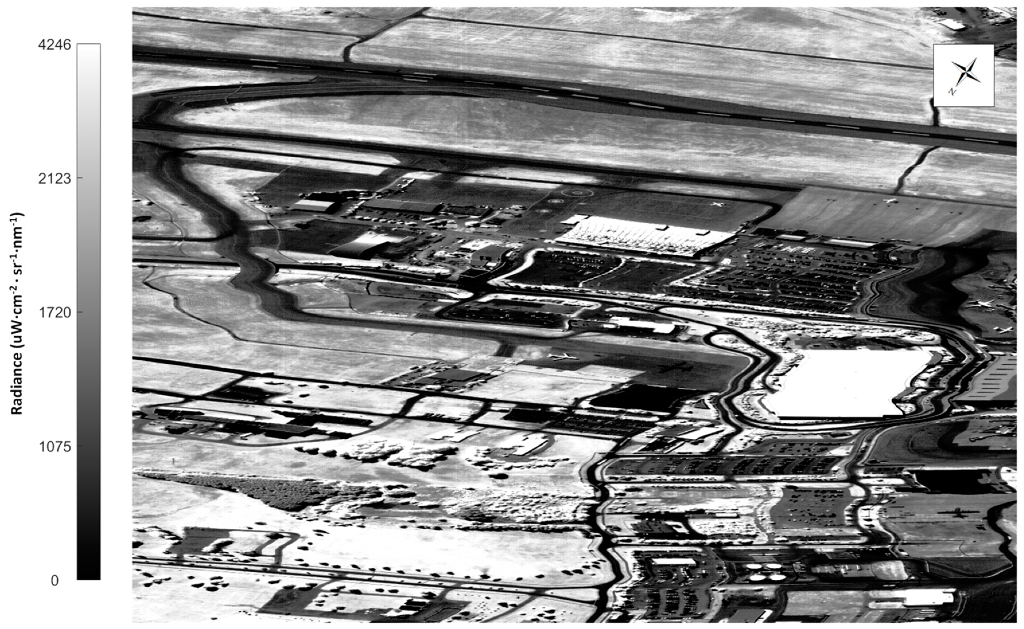
Figure 5.
Non-geocorrected CASI imagery of the data acquisition site. The blue line indicates the ROI selected for the analysis. The ROI contained a single pixel from each column across the asphalt road. Ground calibration measurements were taken on the asphalt surface located by the red X, in accordance with Figure 2.

Figure 6.
Schematic view of the basic algorithm for the application of the CC in the spatial localization of errors in HSI data.
Figure 6.
Schematic view of the basic algorithm for the application of the CC in the spatial localization of errors in HSI data.

Figure 7.
Schematic view of the basic algorithm for the application of the CC in the spectral localization of errors in HSI data.
Figure 7.
Schematic view of the basic algorithm for the application of the CC in the spectral localization of errors in HSI data.

Figure 8.
Schematic view of the basic algorithm for the application of the CC in the localization of finer errors in HSI data.
Figure 8.
Schematic view of the basic algorithm for the application of the CC in the localization of finer errors in HSI data.
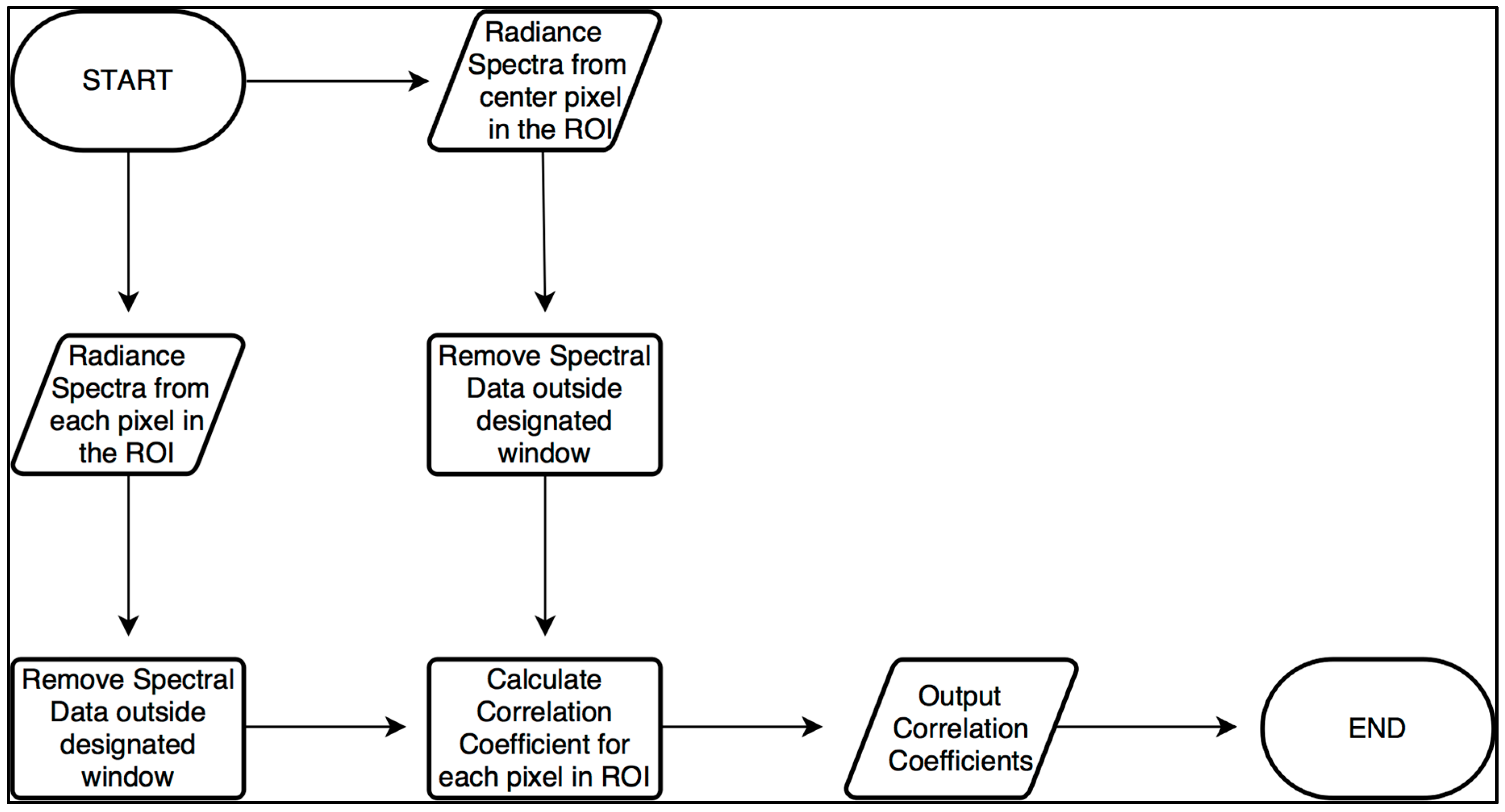
Figure 9.
Averaged and normalized ground spectrum of asphalt before and after interpolation. The differences between the two curves can be seen in the subplot, which zooms in on the 1185–1255 nm spectral window. The interpolated curve, , was used for the methodologies described in Section 2.3. The mean squared error between overlapping data points before and after interpolation was negligible (<10−30). The Akima interpolation method generated a qualitatively smooth .

Figure 10.
The CC between and each of the transformed datasets, . (a) The CC asymptotically reduced from one when the SNR decreased through the introduction of AWGN. (b) The CC was invariant to additive transformations. (c) Multiplicative transformations had no impact on the CC. (d) The introduction of a spectral shift resulted in a small but clear decrease in the CC. (e) The multiplicative transformation of a single feature was detected in the CC by a gradual reduction.

Figure 11.
The CC between and each of the transformed datasets, . All signals were characterized by an SNR value of 100:1. The trends from Figure 10 persisted, despite being masked by the noise to some degree. (a) The CC was invariant to the additive transformation. (b) Multiplicative transformations had no impact on the CC. (c) The introduction of a spectral shift resulted in a small, but clear decrease in the CC. (d) The multiplicative transformation of a single feature was detected in the CC by a gradual reduction.

Figure 12.
The standard deviation of the CCs at various noise levels. There was an asymptotic increase in the standard deviation of the CCs when the SNR decreased through the introduction of AWGN.
Figure 12.
The standard deviation of the CCs at various noise levels. There was an asymptotic increase in the standard deviation of the CCs when the SNR decreased through the introduction of AWGN.

Figure 13.
The CCs calculated across the field-of-view with respect to the entire spectrum from the center pixel. (a) The CC of the CASI imagery (23 June 2016); (b) SASI imagery (23 June 2016); (c) CASI imagery (24 June 2016); (d) SASI imagery (24 June 2016). (a,c) The CASI imagery was characterized by systematic reductions near the edges of the FOV. These revealed potential errors consistent with the spectral smile effect and other cross-track illumination effects. This reduction was most substantial for the CASI images generated by the old processing methodology. Compared to the imagery from the 24th, the CCs were more uniform across the FOV for the CASI data from the 23rd. (b,d) The SASI imagery was consistent across all dates and processing methodologies. There was a notable reduction in the CCs across the FOV from Pixels 548–564. This revealed the spatial location of an error.


Figure 14.
Histogram-equalized CASI image (24 June with the original processing) at 393.068 nm. The asphalt road along the south side of the image was brightest along the edge pixels. The errors in the data are highlighted by the red arrows.
Figure 14.
Histogram-equalized CASI image (24 June with the original processing) at 393.068 nm. The asphalt road along the south side of the image was brightest along the edge pixels. The errors in the data are highlighted by the red arrows.

Figure 15.
Histogram-equalized CASI imagery (24 June with the refined processing) at 393.068 nm. The asphalt road along the south side of the image was brightest along the edge pixels. These errors in the data are highlighted by the red arrows and were less noticeable in the imagery that was generated from the refined processing.

Figure 16.
Histogram-equalized SASI imagery (24 June with the refined processing) at 1003 nm. An error across Pixels 548–564 is identified by the red arrow.
Figure 16.
Histogram-equalized SASI imagery (24 June with the refined processing) at 1003 nm. An error across Pixels 548–564 is identified by the red arrow.

Figure 17.
The CCs calculated across the field-of-view with respect to the spectrum complementary to the windows in Table 3. (a) CASI imagery (23 June 2016); (b) SASI imagery (23 June 2016); (c) CASI imagery (24 June 2016); (d) SASI imagery (24 June 2016). (a,c) The CCs of the CASI imagery increased greatly, especially along the edges, indicating that the error was primarily contained within the spectral regions identified in Table 3. The CASI data from the 23rd were relatively consistent between both processing methodologies. Although this trend generally held for the data from the 24th, (c) showed a notable offset. (b,d) The large reduction in the CCs from the SASI imagery at Pixels 548–564 was not present after removing the problematic band that was found between 993 and 1008 nm.


Figure 18.
The CCs calculated across the field-of-view of the CASI imagery with respect to the spectrum from the center pixel. The wavelength regions used to calculate the CCs are identified in each graph and correspond to the values in Table 4. Plots (a,c,e,g,i) correspond to the CASI data that were processed with the original methodology. Plots (b,d,f,h,j) correspond to the CASI data that were processed with the refined methodology. (a,b) The CCs for the 680–712 nm region were highly variable with a low frequency sinusoidal structure. (c,d) The CCs for the 710–745 nm region were relatively constant across the FOV. A distinct reduction was detected in the CC of a single pixel near the right edge for the imagery processed with the original methodology, but not the refined processing. (e,f) There was a reduction of approximately 0.021 in the CC for the 750–775 nm region near the edges of the FOV. This effect is likely caused by the smile effect or other cross-track illumination effects. (g,h) For the data from the 804–846 nm window of the imagery processed with the original methodology, there were characteristic reductions in the CC greater than 0.05 detected. These reductions revealed potential imaging errors for the spectral window in the following spatial ranges: 256–276, 551–576, 912–936 and 1209–1235. These reductions were not present in the CCs for the image derived with the refined processing. (i,j) In the 883–992 nm region, the CCs were relatively constant across the FOV.


Figure 19.
Histogram-equalized CASI imagery (24 June with the original processing) at 706.4 nm. The image is zoomed in to display Columns 57–513 from left to right. There are “striping” artefacts across the FOV. This ripple is clearly visible near the center of the figure, as indicated by the red arrow.

Figure 20.
Histogram-equalized CASI (24 June with original processing) imagery at 744.653 nm. The image is zoomed in to display Columns 1248–1482 from left to right. The red and orange arrows point to the errors in Pixels 1454 and 1456 in the cross-track, respectively. These errors were visualized as a bright and dark vertical stripe.

Figure 21.
Histogram-equalized CASI imagery (24 June with original processing) at 835.491 nm. The red lines show the locations of distinct “striping” artefacts.
Figure 21.
Histogram-equalized CASI imagery (24 June with original processing) at 835.491 nm. The red lines show the locations of distinct “striping” artefacts.

Figure 22.
Histogram-equalized CASI imagery (24 June with original processing) at 931.099 nm. The imagery is stable, with no obvious errors.
Figure 22.
Histogram-equalized CASI imagery (24 June with original processing) at 931.099 nm. The imagery is stable, with no obvious errors.


Table 1.
The five modifications applied to to generate the transformed signal, .
| Modification | Transformation Model | Data Parameters |
|---|---|---|
| Introduction of Additive White Gaussian Noise | SNR = , | |
| Additive Transformation | ||
| Multiplicative Transformation | ||
| Introduction of Spectral Shift | ||
| Multiplicative Transformation of a Single feature |
Table 2.
The approximate spectral location of known atmospheric absorption features [43]. It is important to note that the wavelength ranges for some atmospheric absorption features may vary in response to external factors. For instance, the range of the water absorption features is highly dependent on water vapor and aerosol optical thickness [44].
| Source | Start Wavelength (nm) | End Wavelength (nm) |
|---|---|---|
| O2 | 686 | 695 |
| H2O | 713 | 734 |
| O2 | 757 | 770 |
| H2O | 806 | 840 |
| H2O | 888 | 997 |
| H2O | 1087 | 1176 |
| O2 | 1223 | 1285 |
| H2O | 1300 | 1521 |
| CO2 | 1591 | 1620 |
| H2O | 1759 | 1982 |
| CO2 | 1991 | 2038 |
| CO2 | 2037 | 2079 |
| CH4 | 2139 | 2400 |
Table 3.
Spatial and spectral localization of large imaging errors. Spatial errors were detected from the data in Figure 13 using the defined threshold. Potential errors were spectrally located through the window-based methodology described in Section 2.4. Errors were detected along the edges of the CASI imagery in the blue end of the spectra. A single band error was detected in the SASI imagery from 993–1008 across Pixels 548–564.
| Imager | Date | Processing | Problematic Pixels | Spectrally-Isolated Range (nm) |
|---|---|---|---|---|
| CASI | 23 June 2016 | Original | 1–70 and 1285–1498 | 366–453 |
| CASI | 23 June 2016 | Refined | 1403–1498 | 396–483 |
| CASI | 24 June 2016 | Original | 1–149 and 1258–1498 | 366–453 |
| CASI | 24 June 2016 | Refined | 1–141 and 1252–1498 | 396–483 |
| SASI | 23 June 2016 | Original | 548–564 | 993–1008 |
| SASI | 23 June 2016 | Refined | 548–564 | 993–1008 |
| SASI | 24 June 2016 | Original | 548–564 | 993–1008 |
| SASI | 24 June 2016 | Refined | 548–564 | 993–1008 |
Table 4.
Identified atmospheric absorption features in the spectral range covered by the CASI.
| Feature Number | Source | Start Wavelength (nm) | End Wavelength (nm) |
|---|---|---|---|
| 1 | O2 | 680 | 712 |
| 2 | H2O | 710 | 745 |
| 3 | O2 | 750 | 776 |
| 4 | H2O | 804 | 846 |
| 5 | H2O | 883 | 992 |
© 2018 by the authors. Licensee MDPI, Basel, Switzerland. This article is an open access article distributed under the terms and conditions of the Creative Commons Attribution (CC BY) license (http://creativecommons.org/licenses/by/4.0/).
Share and Cite
MDPI and ACS Style
Inamdar, D.; Leblanc, G.; Soffer, R.J.; Kalacska, M. The Correlation Coefficient as a Simple Tool for the Localization of Errors in Spectroscopic Imaging Data. Remote Sens. 2018, 10, 231. https://doi.org/10.3390/rs10020231
AMA Style
Inamdar D, Leblanc G, Soffer RJ, Kalacska M. The Correlation Coefficient as a Simple Tool for the Localization of Errors in Spectroscopic Imaging Data. Remote Sensing. 2018; 10(2):231. https://doi.org/10.3390/rs10020231
Chicago/Turabian StyleInamdar, Deep, George Leblanc, Raymond J. Soffer, and Margaret Kalacska. 2018. "The Correlation Coefficient as a Simple Tool for the Localization of Errors in Spectroscopic Imaging Data" Remote Sensing 10, no. 2: 231. https://doi.org/10.3390/rs10020231
Note that from the first issue of 2016, this journal uses article numbers instead of page numbers. See further details here.