Sensitivity Analysis of Arctic Sea Ice Extent Trends and Statistical Projections Using Satellite Data


1
Cooperative Institute for Climate and Satellites-North Carolina (CICS-NC) at NOAA’s National Centers for Environmental Information (NCEI), North Carolina State University, Asheville, NC 28801, USA
2
Department of Computer Science, University of North Carolina at Chapel Hill, Chapel Hill, NC 27514, USA
*
Author to whom correspondence should be addressed.
Remote Sens. 2018, 10(2), 230; https://doi.org/10.3390/rs10020230
Submission received: 30 November 2017
/
Revised: 12 January 2018
/
Accepted: 30 January 2018
/
Published: 2 February 2018
(This article belongs to the Special Issue Cryospheric Remote Sensing II)
Abstract
:An ice-free Arctic summer would have pronounced impacts on global climate, coastal habitats, national security, and the shipping industry. Rapid and accelerated Arctic sea ice loss has placed the reality of an ice-free Arctic summer even closer to the present day. Accurate projection of the first Arctic ice-free summer year is extremely important for business planning and climate change mitigation, but the projection can be affected by many factors. Using an inter-calibrated satellite sea ice product, this article examines the sensitivity of decadal trends of Arctic sea ice extent and statistical projections of the first occurrence of an ice-free Arctic summer. The projection based on the linear trend of the last 20 years of data places the first Arctic ice-free summer year at 2036, 12 years earlier compared to that of the trend over the last 30 years. The results from a sensitivity analysis of six commonly used curve-fitting models show that the projected timings of the first Arctic ice-free summer year tend to be earlier for exponential, Gompertz, quadratic, and linear with lag fittings, and later for linear and log fittings. Projections of the first Arctic ice-free summer year by all six statistical models appear to converge to the 2037 ± 6 timeframe, with a spread of 17 years, and the earliest first ice-free Arctic summer year at 2031.
1. Introduction
Since satellite-based measurements became available in the late 1970s, a 10–15% per decade decrease in the annual Arctic sea ice extent (SIE) minimum has been recorded, as measured by the area within the 15% sea ice fraction contour (e.g., [1,2,3,4]). By 2012, a 49% sea ice reduction in extent, relative to the 1979–2000 climatology, was also observed [2,5]. This loss of Arctic ice is occurring at a rate faster than what climate models with enhanced greenhouse gas forcing have predicted [6] and steeper than at any time since 1850 [7]. In addition, the sea ice winter build-up has been setting record lows for the last three years in a row [8]. Sea ice thinning, as a result of multiyear sea ice loss [9,10], further accelerates this Arctic sea ice depletion process, increases nonlinearity variability of Arctic sea ice coverage, and therefore reduces its predictability.
With this rapid and accelerated Arctic sea ice loss, ice-free Arctic summer—because of its pronounced impact on global climate, coastal habitats, national security, and the shipping industry [11,12]—has become a renewed interest of many studies. An ice-free or nearly ice-free Arctic Ocean is often defined as having less than one million square kilometers of sea ice coverage (e.g., [5]), because it is very difficult to melt the thick ice around the Canadian Arctic Archipelago. Using September SIE as the indicator and the ice-free threshold of one million square kilometers, Overland and Wang [5] examined three commonly used approaches for estimating the timing of the first ice-free Arctic summer: (1) extrapolation of sea ice volume data; (2) stochastic projection, assuming several more rapid loss events such as 2007 and 2012; and (3) projection of climate models. These three approaches have roughly predicted the first ice-free Arctic summer year (FIASY) to be 2020 or earlier, 2030 with a 10-year margin of error, and 2040 or later, respectively. They have also confirmed that climate models in CMIP5 tend to be conservative in their sea ice projections.
The current time series of Arctic SIE are mostly computed from sea ice concentration estimates derived from satellite measurements using passive microwave sensors from the Defense Meteorological Satellite Program (DMSP), as in [1,2]. These sea ice concentration estimates are accurate for ice area fraction values that are at about 15% or higher in a given grid cell with spatial resolution ranging from 12.5 to 35 km. Therefore, the estimated time frame for ice-free grid cells is only relevant to this particular accuracy and resolution. In addition, multiple types of sensors from multiple missions are utilized to formulate the long-term time series of sea ice concentration, and trends could be impacted by bias induced by these different sensors (e.g., [1,2,13]). Therefore, it is beneficial to compute the SIE time series from an inter-calibrated satellite sea ice concentration product.
The observation-based SIE trends and projections are often based on the least squares fit and extrapolation of a given statistical model function. This approach tends to be sensitive to initial and ending values, as well as the length of the time series (see for more discussion on reference values and climatological periods [14]). It is also highly influenced by variability of the time series, especially outliers such as those associated with extreme events. The projection of when the ice-free summer occurs varies largely with the fitting functions that are used [15]. Utilizing three commonly used fitting methods—linear, quadratic, and exponential—Meier et al. [15] projected the FIASY to be 2101, 2035, and 2065, respectively. In that study, the fitting functions were trained by the satellite sea ice data from 1979 to 2005. They have shown that extending the sea ice data back to 1953 did not change these FIASY projections much.
The satellite sea ice concentration data are commonly available to users as either daily or monthly averages. Daily SIE time series computed from daily concentration data are more likely to be impacted by missing data in satellite observations. Intuitively, trends computed from daily data will also be more prone to the impact of outliers and influenced by short-term fluctuations than trends computed from monthly averages. To help mitigate the impact of missing data and weather-induced fluctuations, the commonly used annual SIE minimums tend to be based on five-day unweighted moving averages of daily SIE values. Long-term SIE trends are usually based on their monthly averages (e.g., https://nsidc.org/data/seaice_index/, accessed 31 March 2017).
In this analysis, we take a systematic look at the statistical sensitivity of Arctic SIE trends and statistical FIASY projections using an inter-calibrated, long-term sea ice concentration data record of 37 years (1979–2015) [3,13]. The questions to be addressed in this work are: How sensitive are decadal linear trends of annual SIE maximums and minimums to different averaging methods and intervals? How sensitive are linear FIASY projections to different data periods and endpoints? How well do commonly used nonlinear statistical models describe the data time series and provide projections for the FIASY?
2. Data and Methods
The NOAA/NSIDC sea ice concentration climate data record (CDR) is derived from measurements taken by the passive microwave sensors onboard the Defense Meteorological Satellite Program (DMSP) F8, F11, and F13, and F17 satellites. The passive microwave sensors include the Scanning Multichannel Microwave Radiometer (SMMR, 1978–1987), the Special Sensor Microwave/Imager (SSM/I, 1987–2007), and Special Sensor Microwave Imager/Sounder (SSMIS, 2008–present). This CDR dataset has been generated by leveraging two well-established sea ice concentration algorithms—NASA Team and Bootstrap—both developed at and produced by the NASA Goddard Space Flight Center (see for more details) [13]. The merged Goddard sea ice concentrations from daily data files are used in this analysis (see for a description of variables in the data files and how to get the data) [3].
The 37 years (1979–2015) of daily sea ice concentration data are used to construct a time series of daily SIEs. SIEs are computed by summing the total area of all cells with a measured sea ice concentration of 15% or higher. The cells within the pole hole region are assumed to be covered with at least 15% of sea ice. This 37-year daily SIE time series is used as the baseline to examine the sensitivity of resultant annual Arctic SIE minimums/maximums to different averaging methods (moving or subsetting average) and time window intervals (5-, 7-, 10-, and 30-day) and the robustness of their linear decadal trends. A moving average in this paper is defined as the unweighted mean of data values within the specified time window which moves forward by one-day increments. Using this averaging method, time windows are overlapping. The subsetting average is also the unweighted mean of data values within the specified time window. However, in this case, the time windows do not overlap; instead, they are adjacent to each other.
There are several types of statistical methods commonly used to compute SIE trends and projections. Commonly used curve fitting models are constructed using either one or a combination of the following functions: polynomial, exponential, and logarithm. The following models are assessed as candidates for describing the annual Arctic SIE minimums:
Exponential:
Gompertz:
Log:
Quadratic:
Linear:
Linear with lag:
where model parameters, αi, i = 1, … 5 were optimized by minimizing the sum of squared errors between the model and data via a simplex-based search approach. The Simplex method is a widely used procedure for linear programming, first proposed by Dantzig in 1947 [16]. It can be used to solve efficiently the optimization of a multivariate cost function by employing a sequence of simplices. Nelder and Mead [17] presented a Simplex algorithm for nonlinear unconstrained optimization. The built-in Nelder–Mead Simplex Method Matlab function from [18] has been utilized in this analysis.
The sensitivity of these statistical curve-fitting methods with regard to several factors, including initial and end values as well as the length and periods of training data, is examined and described in Section 3.3.
3. Results
3.1. Sensitivity to Averaging Methods and Averaging Intervals
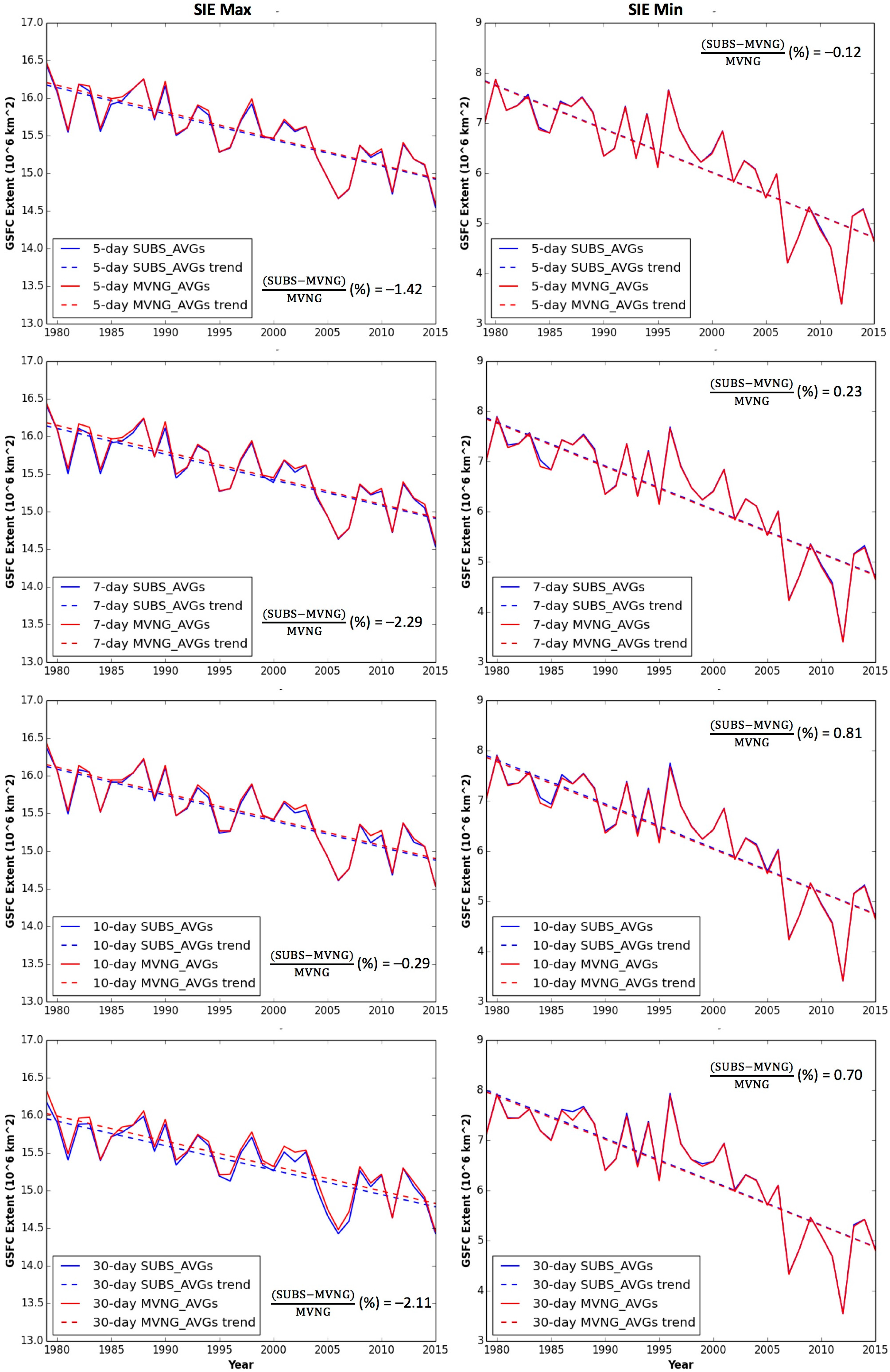
Annual SIE maximums and minimums are commonly used sea ice climate indicators that can be derived from sea ice concentration products. The sensitivity of Arctic SIE trends to averaging methods and intervals is demonstrated by performing linear trend analysis on the time series of averaged annual SIE maximums and minimums. The linear trend line of annual Arctic SIE maximums and minimums for the case of the five-day moving average time series is very close to that of the original daily time series. The subset-averaged maximum/minimum values tend to be slightly reduced/increased as compared to those from moving-averaged (Figure 1). Furthermore, the decadal trends from subsetting averages exhibit slightly higher variability as compared to those from moving averages (Table 1).
The percentage changes of the linear decadal trends relative to the trends of the original daily time series tend to be more variable for the SIE annual maximums than the SIE annual minimums. The linear decadal trends of the SIE annual maximum from 30-day moving and subsetting averages are 4.05% and 6.07% smaller, respectively, relative to that from the original time series (Table 1). This means that applying either averaging technique results in a more conservative sea ice loss trend. The percentage change of the linear decadal trends from of the original time series for SIE annual minimum is very small (less than 0.92%; Table 1).
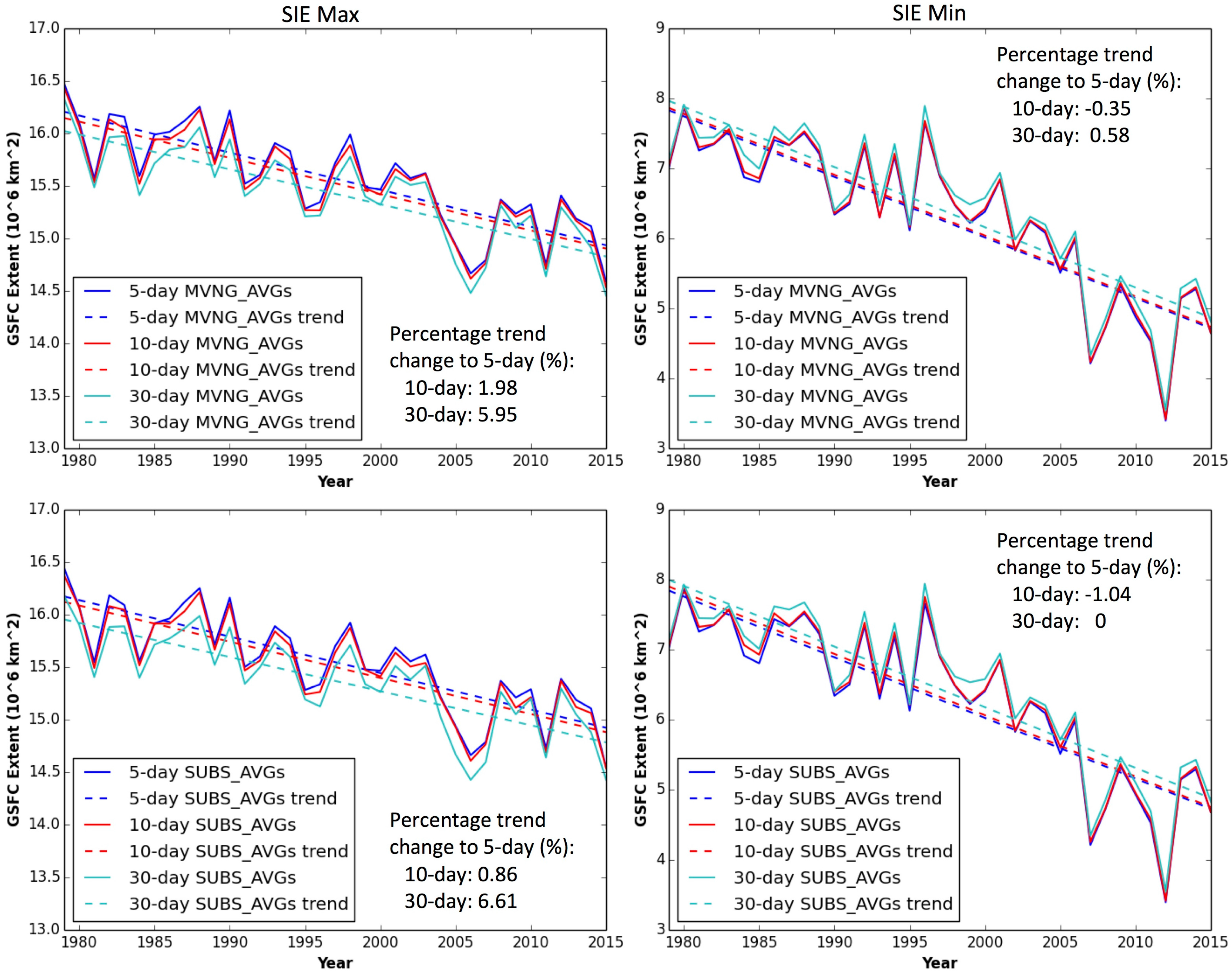
The decadal trend lines from 10-day averages are very close to those of the five-day averages while slight differences are present for those from 30-day averages (Figure 2). Note that the seven-day average case is not included in Figure 2, as its trend lines are between that of the five-day and 10-day averages; however, its statistical attributes are still captured in Table 1.
The percentage changes of the SIE annual maximum decadal trends relative to those from the original daily SIE time series range from about −2.02% to 4.05% for the moving average, and from −0.58% to 6.07% for the subsetting average (Table 1). The percentage changes are much smaller for the SIE annual minimum decadal trends. They range from −0.12% to 0.81% for the moving averages and from −0.92% to 0.12% for the subsetting averages. The same order of sensitivity is found for the decadal trends from the times series from the 10-day and 30-day averaging intervals relative to those of the five-day averaging interval (Figure 2). Relative to the moving averages with the same averaging interval, the percentage changes for the subsetting averages range from −2.29% to –0.29% for the SIE annual maximums, and from 0.12% to 0.81% for annual minimums (Figure 1). Therefore, the overall sensitivity is 6.61%/1.04% or less for the decadal trends of the SIE annual maximums/minimums, respectively.
3.2. Sensitivity of Arctic Ice-Free Projection to Time Domain of Linear Regression
As shown in the previous section, no significant difference amongst trends calculated from 5-, 7-, 10-day and 30-day moving and subsetting averages was found. Since the five-day moving average is a commonly used approach, we will use the SIE annual minimum time series derived from the five-day moving average method for the rest of the analysis. The linear regression trends for different data periods are computed, from which the FIASY is projected. The results are displayed in Figure 3 and summarized in Table 2.
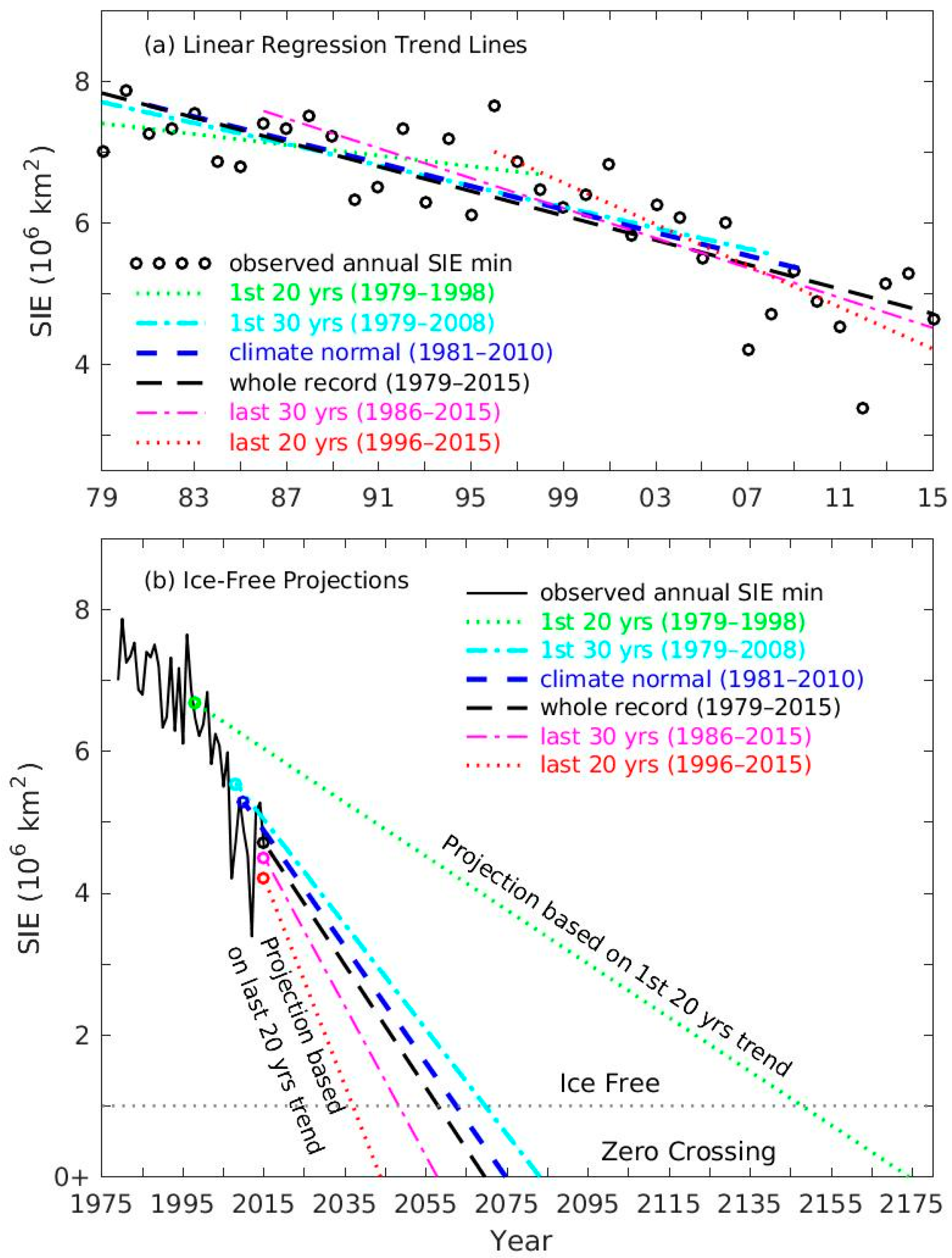
The linear trend for the whole data period (1979–2015) is about −0.87 (106 km2/decade) (Table 2 and Figure 3). Assuming this trend is persistent, the Arctic summer is projected to be ice-free after 2058 (zero-crossing at year 2069). The linear trend from 1996 to 2015 (the last 20 years of the available time series) is about −1.47 (106 km2/decade), which projects the Arctic summer to be ice-free after 2036, in less than 20 years (zero-crossing at year 2043). In comparison, the trend for the current climate normal period (1981–2010) is −0.82 (106 km2/decade), which would result in Arctic ice-free summer beginning at year 2062 (zero-crossing at 2074). The trend of the climate normal period is slightly slower than that based on the trend from the whole record period (1979–2015) as the time period for the climate normal does not include the record low in 2012. On the other hand, the linear trend from the first 20 years of the time series (1979–1998) projects 2147 for ice-free and 2174 for zero-crossing. Therefore, it seems that the accelerated reduction of sea ice extent in the last 20 years (1996–2015) has put the prospect of an ice-free Arctic summer well into our near future. Although all of the above linear trends for the annual SIE minimums are significant at the 99% confidence level, the question is whether any of these linear trends will persist in the future. There is a drastic jump in decadal trends between the first 20 and last 20 years (−0.38 vs. −1.47 106 km2/decade). The acceleration, even in the linear sense, is very distinct and is reflected in the ice-free projections shown in Figure 3. If this trend-acceleration continues, the FIASY could continue to move closer to the present day.
3.3. Sensitivity of Different Statistical Curve Fitting Functions
The linear fitting is the simplest approach. However, visual examination of the SIE annual minimum data presented in Figure 3 suggests that the linear functional form is not appropriate for this application, as the decay in SIE is clearly accelerating in the latter part of the time series.
Statistical curve-fitting models for Arctic sea ice extent and their associated FIASY projections have been previously examined by several studies (e.g., [10,14,15]). In this study, using the same long-term, consistent time series of sea ice data, we compare six commonly used statistical models for this type of application and present the results in Figure 4 and Table 3.
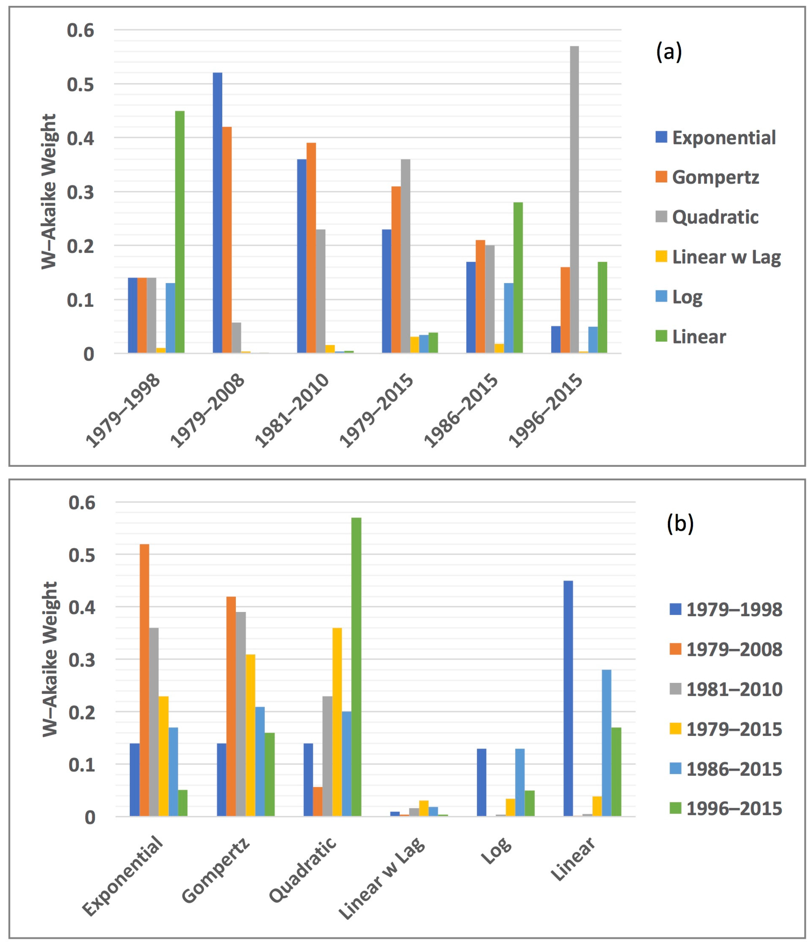
Metrics from model optimization are captured in Table 3, including RMSE (in) (root mean squared errors over data within the time period); RMSE (out) (root mean squared errors over data outside of the training domain (e.g., for the 1979–1998 period, this would be calculated for 1999–2015)); AICc (Akaike information criterion corrected for small sample size); and W-Akaike weights [19,20]. The AICc is a statistically-based means of model selection that estimates the quality of each model in comparison to other models for a given data set, taking into account the number of model parameters and data set sample size. Given a set of AICc values, the optimal model of the sample has the minimum value. W-Akaike weights are derived directly from the AICc values and may be interpreted as the probability that the model is the best of the sample. Note that summing the W-Akaike weights across the sample is 1, and further that the optimal model of the sample has the maximum (probability) value.
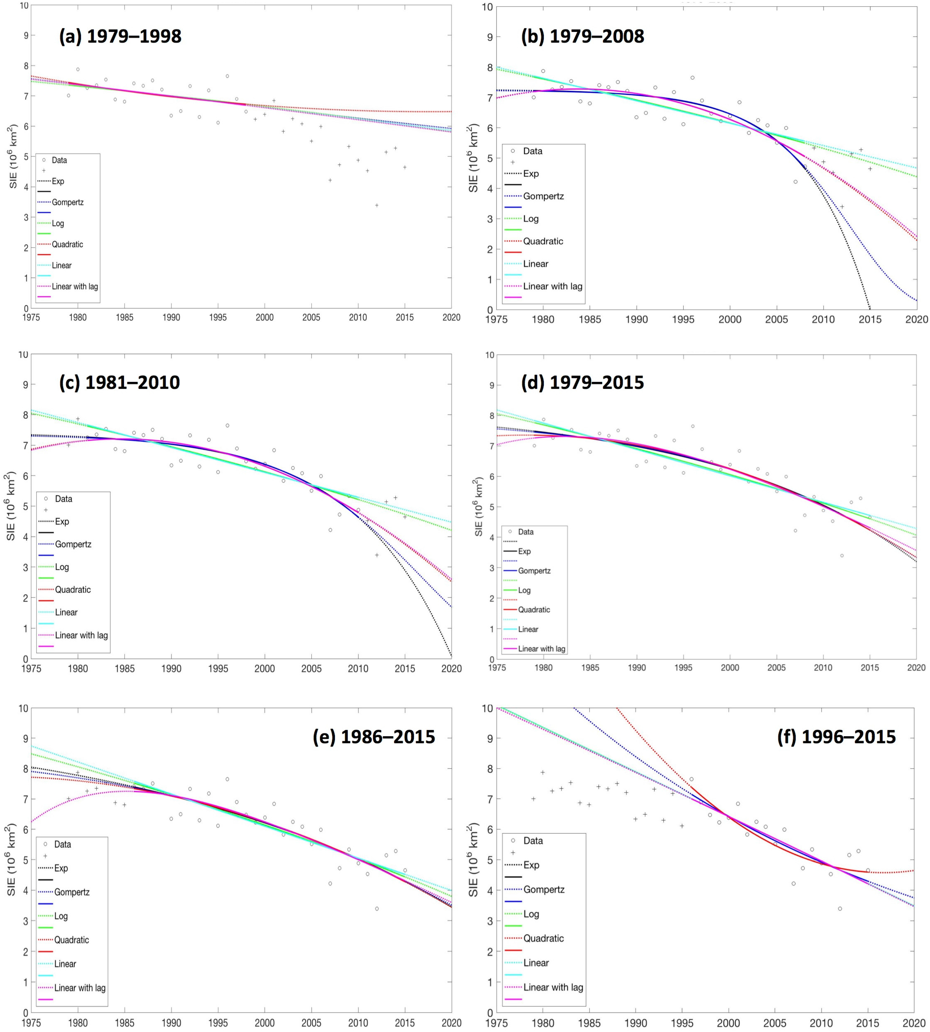
Table 4 and Table 5 summarize the ice-free and zero-crossing projections, respectively, for each of the models as optimized over the 6 different time periods. Note that the Gompertz model will never cross zero, denoted “N/A” in the Table 5 entries. Additionally, when tuned over the first 20 years and the last 20 years, the quadratic model also failed to reach both ice-free and zero-crossing conditions. These cases indicate that, although the model fit data well over the training period, future extrapolation is likely not reliable. Ice-free conditions are projected to occur anywhere from 2014 to beyond 2100. Similarly, zero-crossing is projected to occur anywhere between 2015 to beyond 2100.
Examination of Figure 4a clearly shows that although all are about equally good at representing the period of calibration, none of the models trained over the first 20 years of the time series do a good job of predicting future SIE annual minimums. Mostly they tend to overpredict the sea ice extent; the quadratic model actually projects that SIE will increase over time, which is unlikely given that the data for the final 17 years clearly show a decreasing trend. In Figure 4b, the exponential, Gompertz, quadratic, and linear with lag models all appear to characterize well the domain of calibration, 1979–2008. However, comparing the extrapolated values of 2009–2015 with model predictions shows that none of these four candidate models capture the future behavior well. In particular, the exponential model drops off far too sharply, yielding a prediction of ice-free conditions in 2014, which we know did not occur. These poor predictions are quantitatively reflected in the RMSE (out) value shown in Table 4, which is significantly higher than for the other candidates. Therefore, although this model was selected as best among the candidates for this calibration domain, little faith is held in its ability to project future Arctic sea ice conditions.
The model fits resulting from fitting over the climate normal period of 1981–2010 are shown in Figure 4c. Only two data points not used for calibration are available for comparison in advance of the calibration domain and five data points after it. The quadratic and linear with lag models appear unstable extrapolating into the past. The exponential and Gompertz models appear to underestimate the sea ice extent in the future. The log and linear models do not appear to capture the dynamics of any of the curve that well, which is corroborated by their low W values in Table 3.
In Figure 4d, the entire available time domain is used for calibration, so no inferences may be made about the models’ prediction capabilities. The three best fitting models are the quadratic, Gompertz, and exponential, respectively. However, the quadratic model is known to be unstable in extrapolation regions and given that there is no reserved data to demonstrate otherwise, we assume it cannot be fully trusted to provide reliable predictions.
Using the last 30 years of the time series, 1986–2015, yields models predictions from all candidates that look quite similar during the calibration domain (Figure 4e). It also yields the best overall predictions compared to other periods, reflected by the smaller RMSE values (Table 3). It is therefore not surprising that the linear model, the simplest of all the six candidates, is selected as best using the statistical metrics that take into account and penalize models with greater complexity and the associated larger number of estimated parameters. However, the linear model performs the worst of all candidates in extrapolation as evidenced by the RMSE (out) value in Table 3. Admittedly, this metric only accounts for comparisons taking place in the past (1979–1985) and our more pressing concerns are with the model’s ability to extrapolate into the future. Fitting over the last 20 years, 1996–2015, yields varying results. None of the models fit data not used for calibration well (Figure 4f and Table 3). The quadratic model is particularly unstable for extrapolation in either direction, in part demonstrated by the large RMSE (out) value in Table 3. Therefore, although the associated W value implies it is the most probable candidate for 1996–2015, it cannot be trusted outside of this period.
4. Discussion
Using a consistent long-term daily sea ice time series derived from inter-calibrated satellite measurements, we have first examined the robustness of decadal annual SIE minimum and maximum trends to different temporal averaging methods and intervals. Relative to the linear decadal trend of the whole analysis record period of 1979–2015, only slight sensitivity is seen to the varying averaging methods and intervals—about 6.67%/1.04% or less for annual SIE maximum/minimum trends, respectively, relative to those derived from the original daily SIE time series. Therefore, although the five-day moving average is a commonly used approach for estimating the annual SIE maximum and minimum and associated timing, the monthly average (namely, 30-day subsetting average) SIE may be sufficient for climate monitoring.
An ice-free Arctic summer would have pronounced impacts on global climate, coastal habitats, national security, and the shipping industry. With the rapid and accelerated Arctic sea ice loss that has placed the reality of an ice-free Arctic summer close to the present day, it is important to have an accurate projection of the FIASY for business planning and climate change mitigation. Statistical methods based on the best curve fit to the historical data are some of the most common approaches used in projecting the first occurrence of an Arctic ice-free summer. In the second part of this paper, we have examined the sensitivity and suitability of six commonly used statistical methods in projecting the FIASY, using the time series of the annual SIE minimum from the five-day moving average.
The linear SIE trends based on the historical ice data are statistically significant and the linear fitting is the optimal model for the first 20-year and the last 30-year periods (Table 3, Figure 5a). The projection based on the linear trend over the last 20 years of the time series places the FIASY at 2036, 12 years earlier compared to a projection based on the trend over the last 30 years. However, our trend sensitivity analysis has also demonstrated that, because that rate of sea ice depletion is accelerating, the linear trend is not robust and may not be a good indicator for predicting the Arctic ice-free timeframe.
The linear with lag fitting consistently yields a low W-Akaike weight across all time periods while the Gompertz, quadratic, and exponential fittings appear to be the more probable models (Table 3, Figure 5b). Unfortunately, the accuracy of the quadratic fitting is very unpredictable outside of its original training window, which limits its utility for extrapolation.
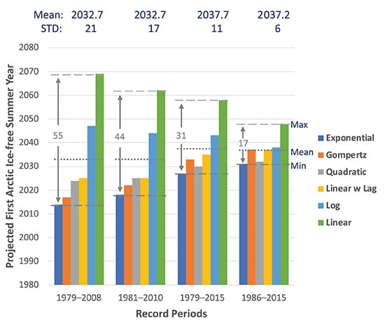
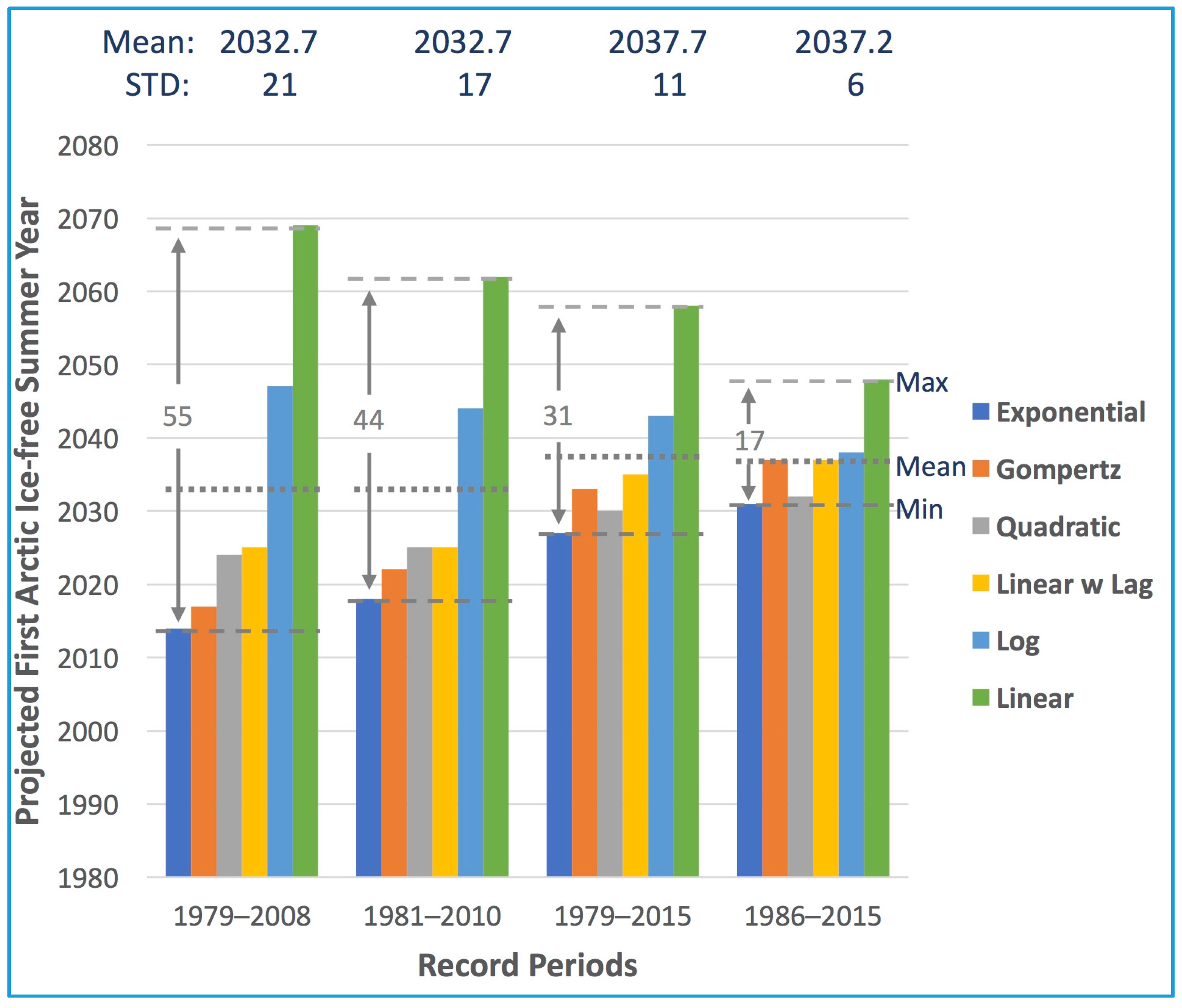
Amongst the six curve fitting models considered with periods of at least 30 years, the FIASY predictions extrapolated from exponential fitting are consistently the earliest, while that of the linear fits are the latest (Table 4, Figure 6). Relative to the means (the average of the projections of all six models), Gompertz, quadratic, and linear with lag fittings are also shown to have earlier predictions of the FIASY, while log fitting is in general later. Figure 6 also shows the reduction in spread from 55 years for the first 30-year period (1979–2008) to 17 years from the last 30-year period (1986–2015). The mean and standard deviation of the projections in the last 30 years are 2037 and 6.
This sensitivity analysis of the FIASY projections is done with a limited number of statistical curve fitting models, using just one dataset. Bearing in mind these limitations, the analysis seems to suggest the convergence of model-projected FIASY to be in the 2037 ± 6 timeframe using the data from the last 30 years (Figure 6). Three out of the six fitting models project the timing to be equal or very close to 2037—Gompertz, linear with the lag, and the log fittings. However, even with a reduced spread, there is still a large uncertainty associated with the individual projected timings, which range from 2031 to 2048. For the same period, the projected zero-crossings range 2035–2057 (Table 5).
It is worth noting that, for the last 20-years data period, four models—exponential, log, linear and linear with lag fittings—have projected the FIASY to be 2036 (Table 4). These four models also projected the zero-crossing summer years to be either 2042 or 2043 (Table 5).
Ironically, the analysis results indicate that the most aggressive and conservative FIASY projections of 2014 and 2048 by the exponential and linear fitting, respectively, are the most probable amongst the all six models for the first/last 30 years (Table 4). (The FIASY projection of 2014 by the exponential fitting for the last 30 years is clearly wrong.) This highlights the challenge of statistically extrapolating a complex and rapidly changing system [15]. The fact that none of the commonly used statistical models are superior in modeling the data in all data periods may also imply that it may be better to use a collective approach such as an ensemble projection using a core set of statistical models. Additionally, although beyond the scope of this paper, a robust characterization of the associated uncertainties originating from the retrieval of the remotely sensed observations and carried through the statistical model fitting of SIE to produce related confidence intervals could also better describe the prediction capacity of the models presented.
5. Conclusions
Using a consistent long-term time series of satellite-based sea ice data, this paper has systematically examined the sensitivity of temporal averaging methods and intervals and the sensitivity of statistical curve fitting methods to different record periods.
The sensitivity of decadal annual SIE maximum/minimum trends to different temporal averaging methods and intervals is found to be less than 6.67% and 1.04%, respectively, relative to those derived from the original daily SIE time series. The sensitivity of six commonly used statistical curve fitting methods to different record periods has demonstrated that none of the six methods are superior in all analyzed periods. The most persistently probable curve-fit model from all the methods examined appears to be Gompertz, even if it is not the best of the subset for all analyzed periods. The FIASY projections based on the fittings from these six models are converging to the time frame of 2037 ± 6, with a spread of 17 years, and the earliest first FIASY projected at 2031.
This analysis does not take into account the different regional declines of SIE, as shown in [15,21,22]. The first ice-free summer year projection is expected to be very variable on the regional scale. This regional variability will be examined in the future. In addition, we intend to use a similar sensitivity analysis approach to explore the nature of SIE simulations and projected changes by climate models. Climate models are thermodynamically consistent and provide additional physical variables that could allow for a better understanding of physical conditions and feedback mechanisms on the Arctic-wide and regional scales. The combination of satellite data, climate model outputs, and a statistical approach may help reach a better estimation about the timing of ice-free situation and its uncertainty.
Acknowledgments
Ge Peng and Jessica Mathews are supported by NOAA’s National Centers for Environmental Information (NCEI) through the Cooperative Institute for Climate and Satellites—North Carolina (CICS-NC) under Cooperative Agreement NA14NES432003. Sensitivity analysis of linear sea ice coverage trend using different averaging methods and intervals was carried out by Jason Yu, initially as a CICS-NC summer intern. Encouragement from and discussions with Otis Brown and Anthony Arguez were beneficial. Ethan Shepherd contributed to the data file aggregation. Tom Maycock has provided beneficial suggestions on the layout of Figure 3 and Figure 6. He also proof-edited the manuscript, which has improved its readability. Comments from Imke Durre, Jake Crouch, and two anonymous reviewers from Remote Sensing have improved the clarity of the paper.
Author Contributions
Ge Peng conceived and designed the experiments. She processed the original data files and computed the Arctic sea ice extent time series used in the sensitivity analysis. She carried out the analysis for decadal linear trends and the first ice-free summer year projections based on these trends. Jason Yu carried out the linear trend sensitivity analysis and generated the graphs used to construct Figure 1 and Figure 2. He also created the annual SIE minimum time series from the five-day moving average. This time series was used in the first ice-free summer year projection sensitivity analysis. Jessica Matthews designed and carried out statistical curve fitting functions sensitivity analysis. The results and graphics from the analysis were used to construct Figure 4 and Figure 5. Ge Peng and Jessica Matthews wrote the draft of the paper. All authors reviewed and contributed to the final manuscript.
Conflicts of Interest
The authors declare no conflict of interest. The founding sponsors had no role in the design of the study; in the collection, analyses, or interpretation of data; in the writing of the manuscript, and in the decision to publish the results.
References
- Comiso, C.J.; Nishio, F. Trends in the sea ice cover using enhanced and compatible AMSR-E, SSM/I, and SMMR data. J. Geophys. Res. 2008, 113, C02S07. [Google Scholar] [CrossRef]
- Cavalieri, J.D.; Parkinson, L.C. Arctic sea ice variability and trends, 1979–2010. Cryosphere 2012, 6, 881–889. [Google Scholar] [CrossRef]
- Peng, G.; Meier, M.N.; Scott, D.J.; Savoie, M. A long-term and reproducible passive microwave sea ice concentration data record for climate studies and monitoring. Earth-Syst. Sci. Data 2013, 5, 311–318. [Google Scholar] [CrossRef]
- Serreze, M.C.; Stroeve, J. Arctic sea ice trends, variability and implications for seasonal ice forecasting. Phil. Trans. R. Soc. 2015, A373. [Google Scholar] [CrossRef] [PubMed]
- Overland, J.E.; Wang, M. When will the summer Arctic be nearly sea ice free? Geophys. Res. Lett. 2013, 40. [Google Scholar] [CrossRef]
- Stroeve, J.C.; Kattsov, V.; Barrett, A.; Serreze, M.; Pavlova, T.; Holland, M.; Meier, W.N. Trends in Arctic sea ice extent from CMIP5, CMIP3 and observations. Geophys. Res. Lett. 2012, 39, L16502. [Google Scholar] [CrossRef]
- Global Climate Change Blog. Historical analysis of Arctic Sea Ice Extent. AccuWeather, 2016. Available online: https://www.accuweather.com/en/weather-blogs/climatechange/historical-analysis-of-arctic/59342719 (accessed on 18 October 2016).
- Thompson, A. Arctic Sea Ice Sets Record-Low Peak for Third Year. Climate Central, 2017. Available online: www.climatecentral.org/news/arctic-sea-ice-sets-record-low-peak-for-3rd-year-21268 (accessed on 30 March 2017).
- Kwok, R.; Untersteiner, N. The thinning of Arctic sea ice. Phys. Today 2011, 64, 36–41. [Google Scholar] [CrossRef]
- Comiso, C.J. Large decadal decline of the Arctic multiyear ice cover. J. Clim. 2012, 25. [Google Scholar] [CrossRef]
- Arctic Climate Impact Assessment (ACIA). Impacts of a Warming Arctic—Arctic Climate Impact Assessment; Cambridge University Press: Cambridge, UK, 2004; 140p. [Google Scholar]
- Intergovernmental Panel on Climate Change (IPCC). Climate Change 2013: The Physical Science Basis. Contribution of Working Group I to the Fifth Assessment Report of the Intergovernmental Panel on Climate Change; Stocker, T.F., Qin, D., Plattner, G.-K., Tignor, M., Allen, S.K., Boschung, J., Nauels, A., Xia, Y., Bex, V., Midgley, P.M., Eds.; Cambridge University Press: Cambridge, UK; New York, NY, USA, 2013; 1535p. [Google Scholar]
- Meier, W.N.; Peng, G.; Scott, D.J.; Savoie, M. Verification of a new passive microwave sea ice concentration climate data record. Polar Res. 2014, 33. [Google Scholar] [CrossRef]
- Wohlleben, T.; Tivy, A.; Stroeve, J.; Meier, W.N.; Fetterer, F.; Wang, J.; Assel, R. Computing and Representing Sea Ice Trends: Toward a Community Consensus. Eos. Trans. AGU 2013, 94, 352. [Google Scholar] [CrossRef]
- Meier, W.N.; Stroeve, J.; Fetterer, F. Whither Arctic sea ice? A clear signal of decline regionally, seasonally and extending beyond the satellite record. Ann. Glaciol. 2007, 46, 428–434. [Google Scholar] [CrossRef]
- Dantzig, G. Origins of the Simplex Method; Tech. Report SOL 87-5; Stanford University: Stanford, CA, USA, 1987. [Google Scholar]
- Nelder, J.A.; Mead, R. A simplex method for function minimization. Comput. J. 1965, 7, 308–313. [Google Scholar] [CrossRef]
- Lagarias, J.C.; Reeds, J.A.; Wright, M.H.; Wright, P.E. Convergence Properties of the Nelder-Mead Simplex Method in Low Dimensions. SIAM J. Optim. 1998, 9, 112–147. [Google Scholar] [CrossRef]
- Cavanaugh, J.E. Unifying the derivations for the Akaike and corrected Akaike information criteria. Stat. Probab. Lett. 1997, 33, 201–208. [Google Scholar] [CrossRef]
- Burnham, K.P.; Anderson, D.R. Model Selection and Multi-Model Inference: A Practical Information-Theoretic Approach, 2nd ed.; Springer: New York, NY, USA, 2002; ISBN 0-387-95364-7. [Google Scholar]
- Boccolar, M.; Parmiggiani, F. Sea-ice area variability and trends in Arctic sectors of different morphology, 1996–2015. Eur. J. Remote Sens. 2017. [Google Scholar] [CrossRef]
- Peng, G.; Meier, W.N. Temporal and regional variability of Arctic sea ice coverage from satellite data. Ann. Glaciol. 2017. [Google Scholar] [CrossRef]
Figure 1.
Time series (solid) of annual Arctic sea ice extent (SIE) maximums (left panels) and minimums (right panels) and their linear trends (dashed) for moving (red) and subsetting (blue) averaging methods. Plots for different time intervals (5-, 7-, 10-, and 30-day) are shown, along with the percentage change of decadal trends. The five-day moving average is a widely adopted method in the cryosphere community, and the 30-day subsetting average is similar to a monthly average.

Figure 2.
Time series (solid) of annual Arctic SIE maximums (left panels) and minimums (right panels) and their linear trends (dashed) for moving average (top two panels) and subsetting average (bottom two panels) methods for different averaging intervals (5-, 10-, and 30-day). The percentage changes of decadal trends from the 10- and 30-day averages relative to that from the five-day averages are displayed.

Figure 3.
(a) Linear regression trend lines based on different subsets of the annual Arctic SIE minimum time series; and (b) Arctic ice-free projections based on these linear trends. The annual Arctic SIE minimum values from five-day moving average based on daily sea ice concentrations are denoted by black circles in (a) and black solid line in (b). Different color and line styles in (a,b) denote the linear regression trend lines and the FIASY projections based on the linear trends for the period of first 20 years (1979–1998; green dotted), first 30 years (1979–2008; cyan dash-dotted), climate normal period (1981–2010; thick blue dashed), all 37 years (1979–2015; black dashed), last 30 years (1986–2015; magenta dash-dotted), and last 20 years (1996–2015; red dotted), respectively. Open circles in (b) denote the end of data fitting and the start of the projection. The horizontal black dotted line in (b) denotes the ice-free threshold of one million square kilometers. The zero-crossing of Arctic SIE minimums is denoted by “0+”, which represents a state in this analysis that all data grid cells in the Arctic Ocean have less than 15% sea ice area fraction.

Figure 4.
Model predictions of annual SIE minimums using different sub-periods of the dataset for training. Circles denote data values used for model training and the predictions over the training set are denoted by solid lines. Plus-signs denote data points excluded from the fitting and dotted lines are the extrapolated predictions based on the resultant fitting. (a) First 20 years (1979–1998); (b) first 30 years (1979–2008); (c) climate normal (1981–2010); (d) the whole record period (1979–2015); (e) last 30 years (1986–2015); and (f) the last 20 years (1996–2015).

Figure 5.
W–Akaike weights: (a) for each data period grouped by statistical models; and (b) for each statistical model grouped by data periods.
Figure 5.
W–Akaike weights: (a) for each data period grouped by statistical models; and (b) for each statistical model grouped by data periods.

Figure 6.
The projected FIASY by six statistical models grouped by time domain of calibration: the first 30 years (1979–2008), the climate normal period (1980–2010), the whole record period (1979–2015), and the last 30 years (1986–2015), respectively. The long-dashed lines denote the minimum and maximum of the projections for each record period. The short-dashed lines denote the mean of the projections for each record period. The values bounded by solid arrow lines denote the spread of the projections. The means and standard deviations of the projected FIASY for each period are noted at the top of the graph.


Table 1.
SIE decadal linear trends (106 km2/decade) from different averaging methods and intervals for the period of 1979–2015, along with their percentage changes relative to those of the original daily SIE time series.
Table 1.
SIE decadal linear trends (106 km2/decade) from different averaging methods and intervals for the period of 1979–2015, along with their percentage changes relative to those of the original daily SIE time series.
| Original | Moving Average Interval (in Days) | Subsetting Average Intervals (in Days) | |||||||
|---|---|---|---|---|---|---|---|---|---|
| 5 | 7 | 10 | 30 | 5 | 7 | 10 | 30 | ||
| SIE Decadal Trends in Annual Maximum (106 km2/decade) | −0.346 | −0.353 | −0.35 | −0.346 | −0.332 | −0.348 | −0.342 | −0.345 | −0.325 |
| Percentage Change to Original (%) | 0 | −2.02 | −1.16 | 0.00 | 4.05 | −0.58 | 1.16 | 0.29 | 6.07 |
| SIE Decadal Trends in Annual Minimum (106 km2/decade) | −0.868 | −0.866 | −0.868 | −0.869 | −0.861 | −0.867 | −0.87 | −0.876 | −0.867 |
| Percentage Change to Original (%) | 0 | 0.23 | 0.00 | −0.12 | 0.81 | 0.12 | −0.23 | −0.92 | 0.12 |
Table 2.
Attributes of linear regressions and projected FIASY and zero-crossing time.
| Case ID | Data Period | Trend (106 km2/Decade) | Margin of Error (106 km2/Decade) * | First Ice-Free Summer (Year) | Zero-Crossing (Year) |
|---|---|---|---|---|---|
| First 20 years | 1979–1998 | −0.38 | 0.19 | 2147 | 2174 |
| First 30 years | 1979–2008 | −0.74 | 0.29 | 2069 | 2083 |
| Climate Normal | 1981–2010 | −0.82 | 0.32 | 2062 | 2074 |
| All years | 1979–2015 | −0.87 | 0.30 | 2058 | 2069 |
| Last 30 years | 1986–2015 | −1.06 | 0.41 | 2048 | 2057 |
| Last 20 years | 1996–2015 | −1.47 | 0.73 | 2036 | 2043 |
* The margin of error in a confidence interval denotes the maximum expected difference between the true and a sample estimate of the statistic. It is proportional to the standard error of the statistic. The margin of error for the linear trend at the 95% confidence level is computed as: ~2 * StdErr, where StdErr denotes the standard error of the linear regression slope.
Table 3.
Metrics from model optimization. Entries in bold indicate the best fit among the six models for the time period.
Table 3.
Metrics from model optimization. Entries in bold indicate the best fit among the six models for the time period.
| Model | Exponential | Gompertz | Log | Quadratic | Linear | Linear w Lag | |
|---|---|---|---|---|---|---|---|
| Period | |||||||
| 1979–1998 (first 20 years) | RMSE (in) (106 km2) | 0.32 | 0.32 | 0.32 | 0.32 | 0.32 | 0.32 |
| RMSE (out) (106 km2) | 0.83 | 0.85 | 0.84 | 0.98 | 0.83 | 0.82 | |
| AICc [(106 km2)2] | −78.61 | −78.62 | −78.46 | −78.69 | −80.99 | −73.39 | |
| W [unitless] | 0.14 | 0.14 | 0.13 | 0.14 | 0.45 | 0.010 | |
| 1979–2008 (first 30 years) | RMSE (in) (106 km2) | 0.39 | 0.39 | 0.46 | 0.41 | 0.47 | 0.41 |
| RMSE (out) (106 km2) | 1.23 | 0.85 | 0.32 | 0.39 | 0.35 | 0.38 | |
| AICc [(106 km2)2] | −62.99 | −62.54 | −50.30 | −58.57 | −51.06 | −53.18 | |
| W [unitless] | 0.52 | 0.42 | 0.00091 | 0.057 | 0.0013 | 0.0039 | |
| 1981–2010 (climate normal) | RMSE (in) (106 km2) | 0.40 | 0.40 | 0.45 | 0.40 | 0.46 | 0.40 |
| RMSE (out) (106 km2) | 0.52 | 0.46 | 0.32 | 0.37 | 0.34 | 0.36 | |
| AICc [(106 km2)2] | −61.25 | −61.43 | −52.25 | −60.40 | −52.79 | −55.10 | |
| W [unitless] | 0.36 | 0.39 | 0.0039 | 0.23 | 0.0052 | 0.016 | |
| 1979–2015 (all years) | RMSE (in) (106 km2) | 0.52 | 0.52 | 0.55 | 0.52 | 0.57 | 0.51 |
| RMSE (out) (106 km2) | N/A | N/A | N/A | N/A | N/A | N/A | |
| AICc [(106 km2)2] | −41.26 | −41.83 | −38.16 | −42.15 | −37.69 | −37.22 | |
| W [unitless] | 0.23 | 0.31 | 0.034 | 0.36 | 0.039 | 0.031 | |
| 1986–2015 (last 30 years) | RMSE (in) (106 km2) | 0.50 | 0.49 | 0.50 | 0.49 | 0.50 | 0.49 |
| RMSE (out) (106 km2) | 0.22 | 0.20 | 0.31 | 0.18 | 0.36 | 0.18 | |
| AICc [(106 km2)2] | −45.31 | −45.64 | −44.66 | −45.58 | −46.23 | −40.76 | |
| W [unitless] | 0.17 | 0.21 | 0.13 | 0.20 | 0.28 | 0.018 | |
| 1996–2015 (last 20 years) | RMSE (in) (106 km2) | 0.41 | 0.40 | 0.41 | 0.38 | 0.41 | 0.41 |
| RMSE (out) (106 km2) | 0.96 | 1.57 | 0.95 | 2.62 | 0.96 | 0.93 | |
| AICc [(106 km2)2] | −59.51 | −61.75 | −59.48 | −64.35 | −61.88 | −54.15 | |
| W [unitless] | 0.051 | 0.16 | 0.050 | 0.57 | 0.17 | 0.0035 |
Table 4.
Projected FIASYs from optimized statistical models. Entries in bold indicate projections from models with the best fit (see AICc and W information from Table 3).
Table 4.
Projected FIASYs from optimized statistical models. Entries in bold indicate projections from models with the best fit (see AICc and W information from Table 3).
| Case ID | Data Period | Exponential | Gompertz | Log | Quadratic | Linear | Linear w Lag |
|---|---|---|---|---|---|---|---|
| First 20 years | 1979–1998 | >2100 | >2100 | 2077 | N/A | >2100 | >2100 |
| First 30 years | 1979–2008 | 2014 | 2017 | 2047 | 2024 | 2069 | 2025 |
| Climate Normal | 1981–2010 | 2018 | 2022 | 2044 | 2025 | 2062 | 2025 |
| All years | 1979–2015 | 2027 | 2033 | 2043 | 2030 | 2058 | 2035 |
| Last 30 years | 1986–2015 | 2031 | 2037 | 2038 | 2032 | 2048 | 2037 |
| Last 20 years | 1996–2015 | 2036 | 2067 | 2036 | N/A | 2036 | 2036 |
Table 5.
Projected first Arctic zero-crossing summer years from optimized statistical models. Entries in bold indicate projections from models with the best fit (see AICc and W information from Table 3).
Table 5.
Projected first Arctic zero-crossing summer years from optimized statistical models. Entries in bold indicate projections from models with the best fit (see AICc and W information from Table 3).
| Case ID | Data Period | Exponential | Gompertz | Log | Quadratic | Linear | Linear w Lag |
|---|---|---|---|---|---|---|---|
| First 20 years | 1979–1998 | >2100 | N/A | 2083 | N/A | >2100 | >2100 |
| First 30 years | 1979–2008 | 2015 | N/A | 2053 | 2027 | 2083 | 2028 |
| Climate Normal | 1981–2010 | 2020 | N/A | 2050 | 2028 | 2074 | 2029 |
| All years | 1979–2015 | 2030 | N/A | 2049 | 2034 | 2069 | 2041 |
| Last 30 years | 1986–2015 | 2035 | N/A | 2044 | 2036 | 2057 | 2044 |
| Last 20 years | 1996–2015 | 2043 | N/A | 2043 | N/A | 2043 | 2042 |
© 2018 by the authors. Licensee MDPI, Basel, Switzerland. This article is an open access article distributed under the terms and conditions of the Creative Commons Attribution (CC BY) license (http://creativecommons.org/licenses/by/4.0/).
Share and Cite
MDPI and ACS Style
Peng, G.; Matthews, J.L.; Yu, J.T. Sensitivity Analysis of Arctic Sea Ice Extent Trends and Statistical Projections Using Satellite Data. Remote Sens. 2018, 10, 230. https://doi.org/10.3390/rs10020230
AMA Style
Peng G, Matthews JL, Yu JT. Sensitivity Analysis of Arctic Sea Ice Extent Trends and Statistical Projections Using Satellite Data. Remote Sensing. 2018; 10(2):230. https://doi.org/10.3390/rs10020230
Chicago/Turabian StylePeng, Ge, Jessica L. Matthews, and Jason T. Yu. 2018. "Sensitivity Analysis of Arctic Sea Ice Extent Trends and Statistical Projections Using Satellite Data" Remote Sensing 10, no. 2: 230. https://doi.org/10.3390/rs10020230
Note that from the first issue of 2016, this journal uses article numbers instead of page numbers. See further details here.