Demonstration of Percent Tree Cover Mapping Using Landsat Analysis Ready Data (ARD) and Sensitivity with Respect to Landsat ARD Processing Level

Abstract

The recently available Landsat Analysis Ready Data (ARD) are provided as top of atmosphere (TOA) and atmospherically corrected (surface) reflectance tiled products and are designed to make the U.S. Landsat archive for the United States straightforward to use. In this study, the utility of ARD for 30 m percent tree cover mapping is demonstrated and the impact of different ARD processing levels on mapping accuracy examined. Five years of Landsat 5 and 7 ARD over 12 tiles encompassing Washington State are considered using an established bagged regression tree methodology and training data derived from Goddard LiDAR Hyperspectral & Thermal Imager (G-LiHT) data. Sensitivity to the amount of training data is examined with increasing mapping accuracy observed as more training data are used. Four processing levels of ARD are considered independently and the mapped results are compared: (i) TOA ARD; (ii) surface ARD; (iii) bidirectional reflectance distribution function (BRDF) adjusted atmospherically corrected ARD; and (iv) weekly composited BRDF adjusted atmospherically corrected ARD. The atmospherically corrected ARD provide marginally the highest mapping accuracies, although accuracy differences are negligible among the four (≤0.07% RMSE) when modest amounts of training data are used. The TOA ARD provide the most accurate maps compared to the other input data when only small amounts of training data are used, and the least accurate maps otherwise. The results are illustrated and the implications discussed.

1. Introduction

Since the opening of the Landsat archive, novel land cover characterization and change detection algorithms have been developed with many focusing on forest mapping [1,2]. Mapping forest/non-forest cover is often straightforward and so sophisticated pre-processing such as atmospheric correction may not be required [3,4,5]. However, the reliable mapping of percent forest cover, forest degradation or recovery, especially over large areas and/or long time periods, requires Landsat pre-processing to improve the radiometric consistency of the data, including atmospheric correction and minimization of bi-directional reflectance effects and flagging or minimization through temporal compositing of clouds and shadows [4,5,6,7,8,9,10,11]. Recently, the United States Geological Survey (USGS) Earth Resources Observation and Science (EROS) Center (Sioux Falls, SD, USA) made available Landsat Analysis Ready Data (ARD) for the conterminous United States (CONUS) that provides top of atmosphere (TOA) and atmospherically corrected (surface) Landsat reflectance data in a tiled format with cloud and shadow masks that are designed for large-area and long-term analyses [12]. This study examines the suitability of ARD for percent tree cover mapping and the sensitivity of the results to the ARD processing level. Five years of Landsat 5 Thematic Mapper (TM) and Landsat 7 Enhanced Thematic Mapper Plus (ETM+) ARD over the state of Washington, which contains forested mountainous regions that are challenging to classify, are considered.

The purpose of this study is to compare the impact of different ARD processing levels on percent tree cover mapping accuracy and not to compare different mapping algorithms. An established Landsat percent tree mapping methodology based on regression tree processing of multi-temporal metrics extracted from Landsat spectral bands [5] is used. The reference data needed to train the regression tree and to assess mapping accuracy are derived from Goddard LiDAR Hyperspectral & Thermal Imager (G-LiHT) data [13]. Sensitivity to the amount of training data is examined because although mapping accuracy generally increases with training set size [14,15], this will depend in an unknown way a priori on the satellite data, data pre-processing, and algorithms that are used [16,17]. Percent tree cover maps derived using the same training data and multi-temporal metrics extracted from four different ARD processing levels are considered and assessed using standard quantitative accuracy measures. Two of the processing levels are the publically available TOA and surface reflectance ARD. In addition, the surface reflectance ARD corrected to minimize bi-directional effects using a semi-physically based bidirectional reflectance distribution function (BRDF) adjustment approach developed for Landsat [18] and also Sentinel-2 [19], as well as weekly composites, are considered. The weekly compositing algorithm is based on the same algorithm used to generate global coverage Web-Enabled Landsat Data (WELD) products, which are publically available [20], and is designed to preferentially select surface observations with minimal cloud, snow, and atmospheric contamination [9].

2. Data and Study Area

2.1. Landsat Analysis Ready Data (ARD)

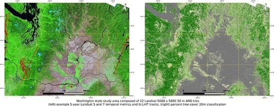
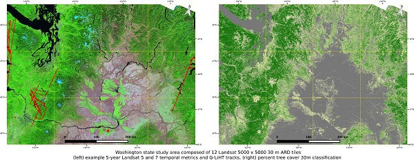
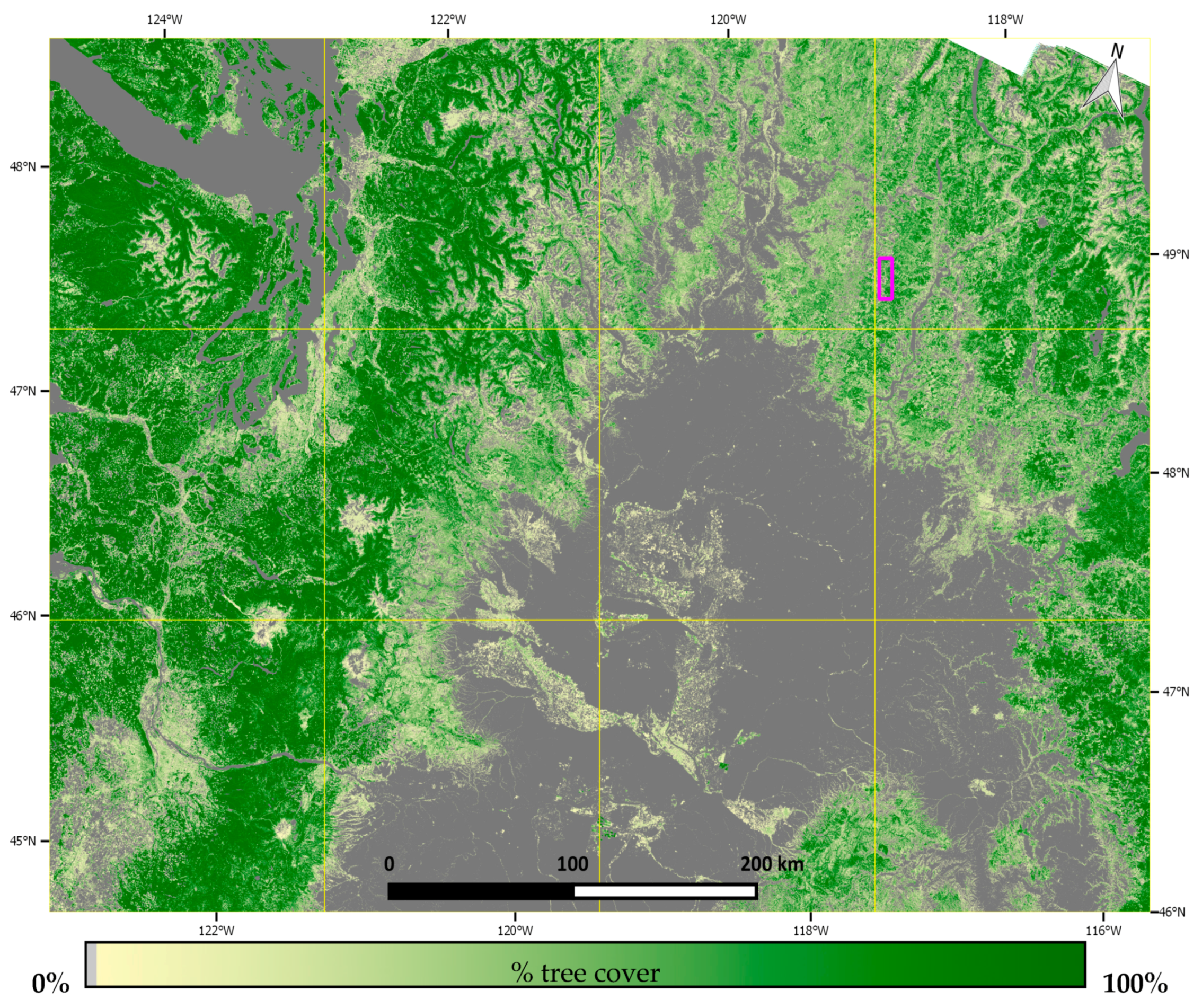
The Collection 1 Landsat ARD were used in this study. The U.S. Landsat archive was reprocessed recently (2017) into a tiered data Collection 1 structure. The Collection 1 products are defined in the heritage 185 km × 180 km Worldwide Reference System (WRS-2) of path (ground track parallel) and row (latitude parallel) scene coordinates in the Universal Transverse Mercator (UTM) projection [21] with a number of new metadata, including angle coefficients, that may be used to derive per-pixel solar and viewing geometry, and per-pixel saturation status, cloud, cloud shadow, cirrus cloud, and snow masks [22]. The Landsat Collection scheme is similar to that adopted for the MODIS land product reprocessing [23] and, for example, the Landsat archive is planned to be reprocessed as a Collection 2 to improve the absolute geolocation accuracy [24].

All of the Collection 1 Landsat data have been processed over the CONUS, Hawaii and Alaska into an ARD tiled format [12]. The CONUS ARD tile structure is the same as that used to generate the CONUS Web-Enabled Landsat Data (WELD) products [9]. Each orbit of Landsat data is stored in non-spatially overlapping, fixed 5000 × 5000 30 m pixel tiles in the Albers equal area projection. Importantly, however, the ARD are generated (projected) directly into the Albers projection and, therefore, are not resampled twice. The ARD tiles are referenced by horizontal and vertical tile coordinates. Each Landsat 4, 5, 7, and 8 sensor has a 15° field-of-view and senses a 185 km swath with a 16-day repeat cycle and typically 22 or 23 overpasses of a fixed location per year are acquired, although the number of surface observations is reduced due to cloud cover over much of the CONUS at the time of Landsat overpass [25,26]. In this study, Landsat 5 TM and Landsat 7 ETM+ ARD were used. These sensors are in the same orbit but are offset by 8 days. The western and eastern sides of a sensor acquisition are overlapped by the eastern and western sides, respectively, of the other sensor acquisition, and are acquired with a one-day separation [18]. Thus, in a week there may be no, one (Landsat 5 or Landsat 7), or two (Landsat 5 and Landsat 7) observations for each ARD tile pixel.

ARD are available as both TOA and atmospherically corrected (surface) reflectance with the Collection 1 per-pixel saturation status, cloud, cloud shadow, cirrus cloud, and snow masks, and also with additional per-pixel views and solar geometry information. The Landsat 4, 5, and 7 ARD are atmospherically corrected using the Landsat Ecosystem Disturbance Adaptive Processing System (LEDAPS), which uses aerosol characterizations derived independently from each Landsat Collection 1 image, assumes a fixed continental aerosol type, and uses ancillary water vapor and ozone data [27]. In this study, both the TOA ARD and surface ARD for Landsat 5 TM and Landsat 7 ETM+ were used. Landsat Bands 3 (center wavelength for both sensors ~0.66 μm), 4 (~0.83 μm), 5 (~1.65 μm), and 7 (~2.22 μm) were used. The blue (~0.49 μm) and green bands (~0.56 μm) were excluded because they are sensitive to atmospheric scattering and are not reliably atmospherically corrected [28,29].

2.2. Study Area

Twelve ARD tiles encompassing the state of Washington (Figure 1) were used. All of the available Landsat 5 TM and Landsat 7 ETM+ ARD from 2006 to 2010 were considered. These five years were selected as both sensor data were available and the Landsat 5 orbit was quite stable compared to previous years when the orbit was not maintained [30]. Only data from weeks 16 (start date 15 April) to 46 (end date 17 November) were used to capture phenological differences over the growing seasons and to avoid periods of winter snow and frequent cloud at the time of Landsat overpass [25,31]. The study area is dominated by forest cover. The western and central northern parts of the state (h03v01, h03v02, h03v03, h04v01, h04v02) have a mild wet climate that is favorable for tree growth, particularly coniferous forests of Douglas fir, western hemlock, and Pacific red cedar [32]. The Olympic Mountains and Cascade Range cross the study area from north to south along the west coast and have an annual precipitation of about 381 cm in the Olympics and 279 cm in the Cascades [33]. The eastern slopes of the Cascades are in a rain shadow and are covered predominantly by dry Ponderosa pine forests [32]. Most of the lowland plains of the Columbia Basin (h05v02, h04v03, h05v03) are in the rain shadow of the Cascades and are treeless and dominated by shrublands, croplands, and pastoral agriculture [34]. The eastern Washington forests (h05v01, h06v01, h06v02, h06v03) are predominantly Rocky Mountain types with Ponderosa pine characterizing the forests at lower elevations and subalpine fir at higher elevations [32].

2.3. Percent Tree Cover 30 m Reference Data Derived from Airborne LiDAR

Goddard LiDAR, Hyperspectral & Thermal Imager (G-LiHT) data were used to derive percent tree cover data needed for training and validation. The G-LiHT sensor package provides simultaneous measurement of vegetation attributes (structure, foliar spectra and brightness temperature) at very high spatial resolution (~1 m) from a range of airborne platforms [13]. The 1 m gridded G-LiHT canopy height model (CHM) product—derived by selecting the maximum 1.5 µm LiDAR return height defined in 1-m grid cells [35]—was used. The 1 m CHM data were reprojected into the ARD projection and then the portion of canopy height ≥5 m within each ARD 30 m pixel was derived to provide an independent estimate of the 30 m pixel percent tree cover. The 5 m height threshold was used as it is a standard forest definition [36,37]. About 2021 square km of G-LiHT flight data acquired from 2012 to 2014 over predominantly mountainous terrain were initially considered (Figure 1, red lines). Of these data, about 80% had no valid CHM data and were not used. A total of 339,153 30 m percent tree cover reference pixels were derived.

3. Methods

3.1. Additional ARD Processing

3.1.1. Weekly Composite Generation

The development of temporal composites that attempt to select the “best” available pixel over a specific reporting period to reduce data volume and improve data consistency has a long heritage [9,38,39,40,41]. In this study, weekly ARD composites were generated by selecting for each ARD 30 m pixel location the Landsat 5 TM or Landsat 7 ETM+ observation acquired in that week that had reduced atmospheric contamination, cloud, and shadow. The compositing approach was based on the original WELD approach [9] that relies on conventional maximum normalized difference vegetation index (NDVI) and maximum brightness temperature criteria, which are used because clouds and aerosols typically depress NDVI and brightness temperature over land [38,39]. Each week of TOA, Landsat 5 TM and Landsat 7 ETM+ ARD were composited together rather than independently. The TOA, rather than the atmospherically corrected ARD, were composited because the atmospheric correction is imperfect, particularly over deserts where there are no dense dark vegetation targets needed for the aerosol retrieval, under certain high aerosol load conditions, and in regions of cloud and relief shadow [28,42]. Surface reflectance weekly ARD composites were derived by replacing each TOA composited reflectance value with the atmospherically corrected band equivalent. The computational approach and data structure to undertake this replacement are described in [29]. Global coverage WELD Landsat data composited in this manner, but not using ARD input, are publically available [20].

3.1.2. BRDF Adjustment

Landsat BRDF effects are often visually apparent [4,43] and view zenith BRDF effects have been documented to be non-negligible and as great as 0.02 and 0.06 (reflectance units) in the Landsat visible and NIR bands, respectively [18]. Rather than using empirical solutions to minimize BRDF effects, which require the presence of similar land cover types or pseudo-invariant features located across each image that are sometimes unavailable [4,44], a semi-physically based BRDF adjustment approach was used. Specifically, the Landsat reflectance for each sensor band at each ARD pixel was adjusted to a nadir view (0° view zenith) and the observed solar zenith to provide Landsat nadir BRDF-adjusted reflectance (NBAR). A c-factor approach was used that is based on multiplying the Landsat reflectance with the ratio of the reflectances modeled using MODIS BRDF spectral model parameters for the observed Landsat and for a nadir view and a specified solar zenith [18]. A fixed set of global average MODIS BRDF spectral model parameters were used as the BRDF shapes of different terrestrial surfaces are similar over the narrow 15° Landsat field of view [18]. The BRDF adjustment was applied to the surface reflectance ARD and to the weekly composited surface reflectance.

3.2. Percent Tree Cover Mapping

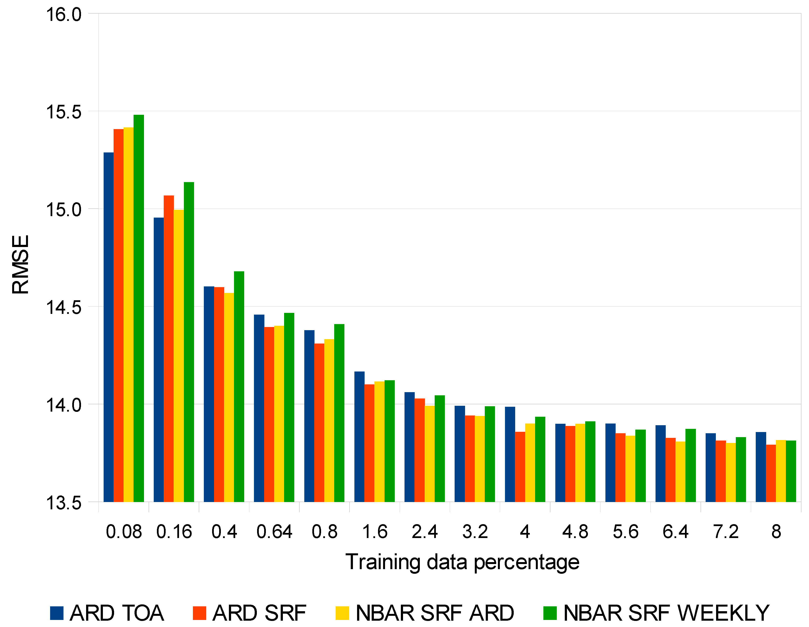
Regression trees are a hierarchical non-parametric method used to predict continuous dependent variables by recursively partitioning the data into more homogeneous subsets [45,46]. Bagged regression trees are an established approach to estimate percent tree cover and are widely used when applied to multi-temporal metrics extracted from Landsat time series [5,40,44]. Multi-temporal metrics, such as the median and other percentile values, capture vegetation phenology but are generally insensitive to the timing of phenological differences across large areas, and are generally insensitive to missing data. Handling missing data is important because Landsat time series have gaps due to cloud cover [47], variable Landsat acquisition frequency [48], and sensor issues [49].

Bagged regression tree mapping was undertaken independently using multi-temporal metrics extracted from four different ARD processing levels, namely the (i) top of atmosphere ARD; (ii) atmospherically corrected ARD; (iii) BRDF adjusted atmospherically corrected ARD; and (iv) weekly composited BRDF adjusted atmospherically corrected ARD. For brevity, we refer to these four processing levels as TOA ARD, SRF ARD, NBAR SRF ARD, and NBAR SRF WEEKLY, respectively. For each processing level, multi-temporal metrics were extracted from the five years of growing season data (years 2006–2010, weeks 16–46). Specifically, at each 30 m pixel location, the 10th, 25th, 50th (i.e., median), 75th, and 90th percentiles of Landsat bands 3, 4, 5, and 7 were extracted. This provided five spatially explicit metrics per band (Figure 1 shows the 50th percentiles of three of the atmospherically corrected ARD bands). In addition, based on our previous Landsat land cover mapping research [4,31,50], the percentiles of spectral band ratios were also derived: (4 − 3)/(4 + 3), (5 − 3)/(5 + 3), (7 − 3)/(7 + 3), (5 − 4)/(5 + 4), (7 − 4)/(7 + 4), (7 − 5)/(7 + 5). In total, 50 metrics were extracted (five percentiles for each of the 4 spectral bands, and five percentiles for each of the 6 spectral band ratios).

The G-LiHT-derived 30 m percent tree reference pixels were randomly divided into two portions with ~80% (271,316) used to build regression tree models and the remaining ~20% (67,837) set aside for validation. The regression tree models were defined using the percent tree reference data as the response variable and the 50 metrics as the explanatory variables. The 50 metrics were extracted using the same reference data locations from the (i) TOA ARD; (ii) SRF ARD; (iii) NBAR SRF ARD; and (iv) NBAR SRF WEEKLY data to generate four sets of regression trees and so four mapped results. The regression trees were generated in a similar manner as [17,31,51]. Specifically, 25 trees were derived with tree growth terminated when additional splits decreased the model deviance by less than 0.001 of the root node deviance. Each 30 m pixel was processed 25 times and the final result was defined as the median of the 25 tree results. Sensitivity to the amount of training data was examined by selecting at random 0.08%, 0.16%, 0.4%, 0.64%, 0.8%, 1.6%, 2.4%, 3.2%, 4%, 4.8%, 5.6%, 6.4%, 7.2%, and 8% per tree of the 271,316 reference data.

The accuracy of each map was evaluated by comparison with the 67,837 G-LiHT-derived 30 m percent tree reference data. Two accuracy metrics were considered: the standard Pearson’s correlation coefficient (r) with a probability of type I error (p-value) and the root mean square error (RMSE) defined as:

$$r=\frac{{{\displaystyle \sum }}_i^n(v_i-\overline{v})\left(y_i-\overline{y}\right)}{\sqrt{{{\displaystyle \sum }}_i^n{\left(v_i-\overline{v}\right)}^2{{\displaystyle \sum }}_i^n{\left(y_i-\overline{y}\right)}^2}}$$

(1)

$$RMSE=\sqrt{\frac{{{\displaystyle \sum }}_i^n{\left(v_i-y_i\right)}^2}{n}}$$

(2)

where v_i is the percent tree cover for validation reference data i, y_i is the corresponding regression tree mapped percent tree cover, $\overline{v}$ and $\overline{y}$ are their mean values, and there are a total of n = 67,837 validation 30 m reference data. Pearson’s correlation coefficient is bounded (−1 ≤ r ≤ 1) and measures the linear correlation between the mapped and validation values where 1 is positive linear correlation, 0 is no linear correlation, and −1 is negative linear correlation. The RMSE provides a more physically interpretable accuracy measure as it reports the difference between the mapped and validation data in percent tree cover units. A perfect map will have RMSE = 0 and r = 1.

4. Results

Figure 2 and Figure 3 show Pearson’s correlation coefficient (r) and the root mean square error (RMSE) accuracy results, respectively. The two accuracy metrics reveal similar results. The mapping accuracy increased as more training data were used. The correlations were all significant (p < 2.2 × 10⁻¹⁶) and increased from 0.9186 (ARD TOA), 0.9174 (ARD SRF), 0.9173 (NBAR SRF ARD), and 0.9169 (NBAR SRF WEEKLY) using the smallest (0.08%) amount of training per tree to 0.9339, 0.9345, 0.9343, and 0.9342, respectively, when the greatest amount (8%) of training per tree was used. Similarly, the RMSE values decreased from 15.29% (ARD TOA), 15.41% (ARD SRF), 15.42% (NBAR SRF ARD), and 15.48% (NBAR SRF WEEKLY) with the smallest (0.08%) amount of training per tree to 13.86%, 13.79%, 13.82%, and 13.81%, respectively, when the greatest amount (8%) of training per tree was used.

The resulting maps based on the TOA ARD were more accurate than the ones based on the other processing levels when sparse training data (≤0.16% per tree) were used and were the least accurate when the most training data were used. The maps based on ARD SRF and NBAR SRF ARD were the most accurate when more training data were used, particularly when ≥0.64% training data per tree was used. However, the mapped differences among the four processing levels were very small—in the third decimal place for the r values and only tenths and hundredths of a percent for the RMSE values.

Figure 4 illustrates the percent tree cover map with the highest accuracy; that is, derived using the atmospherically corrected ARD (SRF ARD) and 8% training data per tree. The results are geographically plausible. The mapped tree cover in the lowland plains of the Columbia Basin and over water bodies (e.g., the Strait of Juan de Fuca and water bodies around Seattle, in the northwest of the study area) where trees are not expected is very low. The favorableness of the environment for forest development depends primarily, in this region, on rainfall and the mapped percent tree cover is broadly approximated by regional precipitation patterns. Thus, the densest percent tree cover is mapped on the windward (west) sides of the Olympic and Cascade Mountains; conversely, on the leeward (east) rain shadow sides less tree cover is mapped. Similarly, the western sides of the spurs of the Rocky Mountains in the east of the study area have a high percent tree cover.

5. Discussion

The overall mapping accuracies were high with RMSE, less than 16%, and with small differences among the four processing levels. As expected, the accuracies increased as more training data were used due to an increased likelihood of capturing spectral and temporal differences within and among percent tree levels [15,16,17,52]. The accuracy differences were negligible (≤0.07% RMSE) when the most training data (8% per tree) were used. Despite this, there are some patterns in the overall results that are discussed below.

The TOA ARD maps were the most accurate compared to the others when the least training data were used and were the least accurate when the most training data were used. This is likely because of the mountainous relief across the study area that reduced the reliability of the atmospheric correction due to direct/diffuse radiation coupling under shadow and partially shaded conditions (i.e., topographic effects) [53,54]. Use of fewer training data meant that atmospheric correction errors present in the other three processing levels were less likely to be sufficiently captured. Similarly, the NBAR derivation used the ARD viewing angles, which may not accurately capture the true viewing geometry in regions of rapidly changing mountainous relief, which will bias the NBAR derivation [55]. Research to develop new Landsat correction approaches that capture the direct/diffuse light coupling and BRDF effects is recommended, although such approaches will require a high-resolution digital elevation model and should also include corrections for Landsat adjacency effects that can be non-negligible [56,57,58].

When greater amounts of training data were used the SRF ARD had the highest overall percent tree cover estimation accuracies, followed by NBAR SRF ARD, NBAR SRF WEEKLY, and then TOA ARD percent tree cover estimations. The TOA ARD provided the lowest accuracy, likely because atmospheric effects and BRDF effects were not minimized. The SRF ARD and NBAR SRF ARD results were the most similar among the four processing levels. This may be because metrics derived from spectral band ratio metrics were used and spectral band ratios reduce first-order viewing angle BRDF variations [59]. The NBAR SRF WEEKLY percent tree cover estimation accuracies were lower than the NBAR SRF ARD accuracies, which is likely because the weekly compositing process meant that fewer multi-temporal Landsat observations (at most one per week) were considered in the metrics generation. If large data volume processing is a constraint, then, given the marginal accuracy differences reported here, NBAR SRF WEEKLY data are appropriate for mapping purposes; this has been demonstrated at CONUS scale using monthly surface NBAR global WELD products [50].

In summary, the overall accuracy statistics often mask local differences when classifications are compared [17,60,61]. Figure 5 shows detailed percent tree cover estimations derived using the most training data (8% per tree) for the four processing levels. A 7 × 21 km subset is shown that was selected because it (i) includes bare ground as well as forested mountainous land; (ii) is geographically distant from any G-LiHT training data (Figure 1); and (iii) is generally representative of the study area mapping results. The subset is centered at Sherman Peak in the northeast corner of the study area (h06v01) and is covered by mixed conifer forests. There is little difference among the four results. The majority of disagreements occur on north-facing forested slopes where the maps derived using the atmospherically corrected data (SRF ARD, NBAR SRF ARD, and NBAR SRF WEEKLY) tend to be more accurate with higher tree canopy density than the TOA ARD results for the reasons discussed above.

It is well established that satellite-derived tree cover estimates tend to over- and under-estimate tree cover in sparse and densely treed areas, respectively [62,63]. Figure 6 shows the percent tree estimation error plotted as a function of percent tree cover; the colors show the frequency of occurrence of the errors. The results derived using the most training data (8% per tree) for the four processing levels are shown. The figure illustrates how the validation data cover the full range of percent tree cover (0 to 100%). As noted above, there is an over- and under-estimation in the estimated percent tree cover at low and high percent tree cover values, respectively. The majority of errors are less than about 15% in magnitude, which is expected (Figure 3). Importantly, for this study, there are no significant differences in the pattern of errors among the four ARD processing levels.

We note that other supervised algorithms, such as random forest and support vector machine classifiers that are increasingly used for time series classification [10], may provide different results. Similarly, different results may be obtained if other features such as non-linear time series decomposition results [15], rather than multi-temporal metrics, are used. However, given the high accuracies reported in this study, we expect that the broad differences observed among the four sets of results (Figure 2, Figure 3, Figure 5 and Figure 6) will be similar. Although the training data used in this study were derived from a random subset of the G-LiHT data that was small (at most 8% of the G-LiHT data per tree), the accuracies may be inflated due to spatial autocorrelation in the response and predictor variables [64,65]. We note, however, that for each ARD processing level, the training and validation data were selected at the same pixel locations and were used to generate and assess, respectively, the percent tree cover maps and, therefore, any spatial autocorrelation bias will be similar among the levels. In this study, a 5 m height threshold was used as it is a standard forest definition [36,37]. Use of other height thresholds or the introduction of additional percent canopy cover criteria to define the training data may change the accuracy of the reported results.

6. Conclusions

The release of the Landsat ARD reduces the pre-processing effort required to make large-area long time period Landsat percent tree maps. The results of this study demonstrate the utility of the ARD. It was straightforward to process the five years of Landsat 5 TM and 7 ETM+ ARD to generate the reported Washington State results using a conventional bagged regression tree and 50 multi-temporal Landsat metrics. Indeed, the greatest human effort was expended on derivation of the G-LiHT percent tree reference data used for training and validation.

This study compared the impact of different ARD processing levels on mapping accuracy over the state of Washington that is dominated by forested mountainous regions and so is challenging to map. Overall accuracies were high (RMSE < 16%) and with very small differences among the four processing levels considered: namely, (i) top of atmosphere ARD; (ii) atmospherically corrected ARD; (iii) BRDF adjusted atmospherically corrected ARD; and (iv) weekly composited BRDF adjusted atmospherically corrected ARD. The TOA ARD data provided the most accurate percent tree cover maps compared to the other input data when only small amounts of training data were used, and the least accurate maps when more training data were used. Given sufficient training data, the accuracy differences were negligible among the four different input data (≤0.07% RMSE), although the atmospherically corrected ARD provided marginally the highest accuracies. It is unknown if these differences will occur in other locations, particularly in regions with less complex terrain where atmospheric correction and BRDF adjustment approaches will be more reliable.

References

1. Hansen, M.C.; Loveland, T.R. A review of large area monitoring of land cover change using Landsat data. Remote Sens. Environ. 2012, 122, 66–74. [Google Scholar] [CrossRef]
2. Banskota, A.; Kayastha, N.; Falkowski, M.J.; Wulder, M.A.; Froese, R.E.; White, J.C. Forest Monitoring Using Landsat Time Series Data: A Review. Can. J. Remote Sens. 2014, 40, 362–384. [Google Scholar] [CrossRef]
3. Song, C.; Woodcock, C.E.; Seto, K.C.; Lenney, M.P.; Macomber, S.A. Classification and change detection using Landsat TM data: When and how to correct atmospheric effects? Remote Sens. Environ. 2001, 75, 230–244. [Google Scholar] [CrossRef]
4. Hansen, M.C.; Roy, D.P.; Lindquist, E.; Adusei, B.; Justice, C.O.; Altstaat, A. A method for integrating MODIS and Landsat data for systematic monitoring of forest cover and change and preliminary results for Central Africa. Remote Sens. Environ. 2008, 112, 2495–2513. [Google Scholar] [CrossRef]
5. Hansen, M.C.; Potapov, P.V.; Moore, R.; Hancher, M.; Turubanova, S.A.; Tyukavina, A.; Thau, D.; Stehman, S.V.; Goetz, S.J.; Loveland, T.R.; et al. High-Resolution Global Maps of 21st-Century Forest Cover Change. Science 2013, 342, 850–853. [Google Scholar] [CrossRef] [PubMed]
6. Lindquist, E.; Hansen, M.C.; Roy, D.P.; Justice, C.O. The suitability of decadal image data sets for mapping tropical forest cover change in the Democratic Republic of Congo: Implications for the mid-decadal global land survey. Int. J. Remote Sens. 2008, 29, 7269–7275. [Google Scholar] [CrossRef]
7. Potapov, P.V.; Turubanova, S.A.; Tyukavina, A.; Krylov, A.M.; McCarty, J.L.; Radeloff, V.C.; Hansen, M.C. Eastern Europe’s forest cover dynamics from 1985 to 2012 quantified from the full Landsat archive. Remote Sens. Environ. 2015, 159, 28–43. [Google Scholar] [CrossRef]
8. White, J.C.; Wulder, M.A.; Hermosilla, T.; Coops, N.C.; Hobart, G.W. A nationwide annual characterization of 25 years of forest disturbance and recovery for Canada using Landsat time series. Remote Sens. Environ. 2017, 194, 303–321. [Google Scholar] [CrossRef]
9. Roy, D.P.; Ju, J.; Kline, K.; Scaramuzza, P.L.; Kovalskyy, V.; Hansen, M.C.; Loveland, T.R.; Vermote, E.F.; Zhang, C. Web-enabled Landsat Data (WELD): Landsat ETM+ Composited Mosaics of the Conterminous United States. Remote Sens. Environ. 2010, 114, 35–49. [Google Scholar] [CrossRef]
10. Gómez, C.; White, J.C.; Wulder, M.A. Optical remotely sensed time series data for land cover classification: A review. ISPRS J. Photogramm. Remote Sens. 2016, 116, 55–72. [Google Scholar] [CrossRef]
11. Zhu, Z. Change detection using Landsat time series: A review of frequencies, preprocessing, algorithms, and applications. ISPRS J. Photogramm. Remote Sens. 2017, 130, 370–384. [Google Scholar] [CrossRef]
12. U.S. Landsat Analysis Ready Data (ARD). Available online: https://landsat.usgs.gov/ard (accessed on 21 December 2017).
13. Cook, B.D.; Corp, L.W.; Nelson, R.F.; Middleton, E.M.; Morton, D.C.; McCorkel, J.T.; Masek, J.G.; Ranson, K.J.; Ly, V.; Montesano, P.M. NASA Goddard’s Lidar, Hyperspectral and Thermal (G-LiHT) airborne imager. Remote Sens. 2013, 5, 4045–4066. [Google Scholar] [CrossRef]
14. Rogan, J.; Franklin, J.; Stow, D.; Miller, J.; Woodcock, C.; Roberts, D. Mapping land-cover modifications over large areas: A comparison of machine learning algorithms. Remote Sens. Environ. 2008, 112, 2272–2283. [Google Scholar] [CrossRef]
15. Yan, L.; Roy, D.P. Improved time series land cover classification by missing-observation-adaptive nonlinear dimensionality reduction. Remote Sens. Environ. 2015, 158, 478–491. [Google Scholar] [CrossRef]
16. Foody, G.M.; McCulloch, M.B.; Yates, W.B. The effect of training set size and composition on artificial neural network classification. Int. J. Remote Sens. 1995, 16, 1707–1723. [Google Scholar] [CrossRef]
17. Egorov, A.V.; Hansen, M.C.; Roy, D.P.; Kommareddy, A.; Potapov, P.V. Image interpretation-guided supervised classification using nested segmentation. Remote Sens. Environ. 2015, 165, 135–147. [Google Scholar] [CrossRef]
18. Roy, D.P.; Zhang, H.K.; Ju, J.; Gomez-Dans, J.L.; Lewis, P.E.; Schaaf, C.B.; Sun, Q.; Li, J.; Huang, H.; Kovalskyy, V. A general method to normalize Landsat reflectance data to nadir BRDF adjusted reflectance. Remote Sens. Environ. 2016, 176, 255–271. [Google Scholar]
19. Roy, D.P.; Li, J.; Zhang, H.K.; Yan, L.; Huang, H. Examination of Sentinel-2A multi-spectral instrument (MSI) reflectance anisotropy and the suitability of a general method to normalize MSI reflectance to nadir BRDF adjusted reflectance. Remote Sens. Environ. 2017, 199, 25–38. [Google Scholar] [CrossRef]
20. Global Web-Enabled Landsat Data. Available online: https://globalweld.cr.usgs.gov/ (accessed on 13 January 2017).
21. Loveland, T.R.; Dwyer, J.L. Landsat: Building a strong future. Remote Sens. Environ. 2012, 122, 22–29. [Google Scholar] [CrossRef]
22. Landsat Collections. Available online: https://landsat.usgs.gov/landsat-collections (accessed on 21 December 2017).
23. Justice, C.; Townshend, J.; Vermote, E.; Masuoka, E.; Wolfe, R.; Saleous, N.; Roy, D.; Morisette, J. An overview of MODIS Land data processing and product status. Remote Sens. Environ. 2002, 83, 3–15. [Google Scholar]
24. Storey, J.; Roy, D.P.; Masek, J.; Gascon, F.; Dwyer, J.; Choate, M. A note on the temporary mis-registration of Landsat-8 Operational Land Imager (OLI) and Sentinel-2 Multi Spectral Instrument (MSI) imagery. Remote Sens. Environ. 2016, 186, 121–122. [Google Scholar] [CrossRef]
25. Ju, J.; Roy, D.P. The Availability of Cloud-free Landsat ETM+ data over the Conterminous United States and Globally. Remote Sens. Environ. 2008, 112, 1196–1211. [Google Scholar] [CrossRef]
26. Kovalskyy, V.; Roy, D.P. A one year Landsat 8 conterminous United States study of cirrus and non-cirrus clouds. Remote Sens. 2015, 7, 564–578. [Google Scholar] [CrossRef]
27. Masek, J.G.; Vermote, E.F.; Saleous, N.E.; Wolfe, R.; Hall, F.G.; Huemmrich, K.F.; Gao, F.; Kutler, J.; Lim, T.K. A Landsat surface reflectance dataset for North America, 1990–2000. IEEE Geosci. Remote Sens. Lett. 2006, 3, 68–72. [Google Scholar] [CrossRef]
28. Ju, J.; Roy, D.P.; Vermote, E.; Masek, J.; Kovalskyy, V. Continental-scale validation of MODIS-based and LEDAPS Landsat ETM+ atmospheric correction methods. Remote Sens. Environ. 2012, 122, 175–184. [Google Scholar] [CrossRef]
29. Roy, D.P.; Qin, Y.; Kovalskyy, V.; Vermote, E.F.; Ju, J.; Egorov, A.; Hansen, M.C.; Kommareddy, I.; Yan, L. Conterminous United States demonstration and characterization of MODIS-based Landsat ETM+ atmospheric correction. Remote Sens. Environ. 2014, 140, 433–449. [Google Scholar] [CrossRef]
30. Zhang, H.K.; Roy, D.P. Landsat 5 Thematic Mapper reflectance and NDVI 27-year time series inconsistencies due to satellite orbit change. Remote Sens. Environ. 2016, 186, 217–233. [Google Scholar] [CrossRef]
31. Hansen, M.C.; Egorov, A.; Roy, D.P.; Potapov, P.; Ju, J.; Turubanova, S.; Kommareddy, I.; Loveland, T.R. Continuous fields of land cover for the conterminous United States using Landsat data: First results from the Web-Enabled Landsat Data (WELD) project. Remote Sens. Lett. 2011, 2, 279–288. [Google Scholar] [CrossRef]
32. Franklin, J.F.; Dyrness, C.T. Natural Vegetation of Oregon and Washington; General Technical Report PNW Holt Library of Science: Series 3; Oregon State University Press: Corvallis, OR, USA, 1988; Volume 8, p. 452. [Google Scholar]
33. Whiteman, C.D. Mountain Meteorology: Fundamentals and Applications; Oxford University Press: New York, NY, USA, 2000; p. 355. [Google Scholar]
34. Boryan, C.; Yang, Z.; Mueller, R.; Craig, M. Monitoring US agriculture: The US Department of Agriculture, National Agricultural Statistics Service, Cropland Data Layer Program. Geocarto Int. 2011, 26, 341–358. [Google Scholar] [CrossRef]
35. G-LiHT: Goddard’s LiDAR, Hyperspectral & Thermal Imager. Available online: http://gliht.gsfc.nasa.gov (accessed on 21 December 2017).
36. Hansen, M.C.; DeFries, R.S.; Townshend, J.R.G.; Carroll, M.; Dimiceli, C.; Sohlberg, R.A. Global percent tree cover at a spatial resolution of 500 meters: First results of the MODIS vegetation continuous fields algorithm. Earth Interact. 2003, 7. [Google Scholar] [CrossRef]
37. FRA 2000 on Definitions of Forest and Forest Change. Available online: http://www.fao.org/docrep/006/ad665e/ad665e06.htm (accessed on 21 December 2017).
38. Holben, B. Characteristics of maximum-value composite images from temporal AVHRR data. Int. J. Remote Sens. 1986, 7, 1417–1434. [Google Scholar] [CrossRef]
39. Roy, D.P. Investigation of the maximum normalized difference vegetation index (NDVI) and the maximum surface temperature (Ts) AVHRR compositing procedures for the extraction of NDVI and Ts over forest. Int. J. Remote Sens. 1997, 18, 2383–2401. [Google Scholar] [CrossRef]
40. Potapov, P.V.; Turubanova, S.A.; Hansen, M.C.; Adusei, B.; Broich, M.; Altstatt, A.; Mane, L.; Justice, C.O. Quantifying forest cover loss in Democratic Republic of the Congo, 2000–2010, with Landsat ETM + data. Remote Sens. Environ. 2012, 122, 106–116. [Google Scholar] [CrossRef]
41. Hermosilla, T.; Wulder, M.A.; White, J.C.; Coops, N.C.; Hobart, G.W. An integrated Landsat time series protocol for change detection and generation of annual gap-free surface reflectance composites. Remote Sens. Environ. 2015, 158, 220–234. [Google Scholar] [CrossRef]
42. Claverie, M.; Vermote, E.F.; Franch, B.; Masek, J.G. Evaluation of the Landsat-5 TM and Landsat-7 ETM+ surface reflectance products. Remote Sens. Environ. 2015, 169, 390–403. [Google Scholar] [CrossRef]
43. Toivonen, T.; Kalliola, R.; Ruokolainen, K.; Malik, R.N. Across-path DN gradient in Landsat TM imagery of Amazonian forests: A challenge for image interpretation and mosaicking. Remote Sens. Environ. 2006, 100, 550–562. [Google Scholar] [CrossRef]
44. Broich, M.; Hansen, M.C.; Potapov, P.; Adusei, B.; Lindquist, E.; Stehman, S.V. Time-series analysis of multi-resolution optical imagery for quantifying forest cover loss in Sumatra and Kalimantan, Indonesia. Int. J. Appl. Earth Obs. Geoinf. 2011, 13, 277–291. [Google Scholar] [CrossRef]
45. Breiman, L.; Friedman, J.; Olshen, R.; Stone, C. Classification and Regression Trees; Wadsworth and Brooks/Cole: Monterey, CA, USA, 1984. [Google Scholar]
46. Breiman, L. Bagging predictors. Mach. Learn. 1996, 24, 123–140. [Google Scholar] [CrossRef]
47. Kovalskyy, V.; Roy, D.P. The global availability of Landsat 5 TM and Landsat 7 ETM+ land surface observations and implications for global 30 m Landsat data product generation. Remote Sens. Environ. 2013, 130, 280–293. [Google Scholar] [CrossRef]
48. Wulder, M.A.; White, J.C.; Loveland, T.R.; Woodcock, C.E.; Belward, A.S.; Cohen, W.B.; Fosnight, E.A.; Shaw, J.; Masek, J.G.; Roy, D.P. The global Landsat archive: Status, consolidation, and direction. Remote Sens. Environ. 2016, 185, 271–283. [Google Scholar] [CrossRef]
49. Markham, B.L.; Storey, J.C.; Williams, D.L.; Irons, J.R. Landsat sensor performance: History and current status. IEEE Trans. Geosci. Remote Sens. 2004, 42, 2691–2694. [Google Scholar] [CrossRef]
50. Zhang, H.K.; Roy, D.P. Using the 500 m MODIS land cover product to derive a consistent continental scale 30 m Landsat land cover classification. Remote Sens. Environ. 2017, 197, 15–34. [Google Scholar] [CrossRef]
51. Hansen, M.C.; Egorov, A.; Potapov, P.V.; Stehman, S.V.; Tyukavina, A.; Turubanova, S.A.; Roy, D.P.; Goetz, S.J.; Loveland, T.R.; Ju, J.; et al. Monitoring conterminous United States (CONUS) land cover change with Web-Enabled Landsat Data (WELD). Remote Sens. Environ. 2014, 140, 466–484. [Google Scholar] [CrossRef]
52. Foody, G.M.; Mathur, A. Toward intelligent training of supervised image classifications: Directing training data acquisition for SVM classification. Remote Sens. Environ. 2004, 93, 107–117. [Google Scholar] [CrossRef]
53. Tanre, D.; Herman, M.; Deschamps, P.Y. Influence of the background contribution upon space measurements of ground reflectance. Appl. Opt. 1981, 20, 3676–3684. [Google Scholar] [CrossRef] [PubMed]
54. Vermote, E.F.; Kotchenova, S. Atmospheric correction for the monitoring of land surfaces. J. Geophys. Res. 2008, 113. [Google Scholar] [CrossRef]
55. Roy, D.P.; Ju, J.; Lewis, P.; Schaaf, C.; Gao, F.; Hansen, M.; Lindquist, E. Multi-temporal MODIS-Landsat data fusion for relative radiometric normalization, gap filling, and prediction of Landsat data. Remote Sens. Environ. 2008, 112, 3112–3130. [Google Scholar] [CrossRef]
56. Li, F.; Jupp, D.L.; Thankappan, M.; Lymburner, L.; Mueller, N.; Lewis, A.; Held, A. A physics based atmospheric and BRDF correction for Landsat data over mountainous terrain. Remote Sens. Environ. 2012, 124, 756–770. [Google Scholar] [CrossRef]
57. Houborg, R.; McCabe, M.F. Impacts of dust aerosol and adjacency effects on the accuracy of Landsat 8 and RapidEye surface reflectances. Remote Sens. Environ. 2017, 194, 127–145. [Google Scholar] [CrossRef]
58. Franch, B.; Vermote, E.F.; Sobrino, J.A.; Fédèle, E. Analysis of directional effects on atmospheric correction. Remote Sens. Environ. 2013, 128, 276–288. [Google Scholar] [CrossRef]
59. Gao, F.; Jin, Y.; Schaaf, C.B.; Strahler, A.H. Bidirectional NDVI and atmospherically resistant BRDF inversion for vegetation canopy. IEEE Trans. Geosci. Remote Sens. 2002, 40, 1269–1278. [Google Scholar]
60. Khatami, R.; Mountrakis, G.; Stehman, S.V. Mapping per-pixel predicted accuracy of classified remote sensing images. Remote Sens. Environ. 2017, 191, 156–167. [Google Scholar] [CrossRef]
61. Heydari, S.S.; Mountrakis, G. Effect of classifier selection, reference sample size, reference class distribution and scene heterogeneity in per-pixel classification accuracy using 26 Landsat sites. Remote Sens. Environ. 2018, 204, 648–658. [Google Scholar] [CrossRef]
62. Hansen, M.C.; DeFries, R.S.; Townshend, J.R.G.; Marufu, L.; Sohlberg, R. Development of a MODIS percent tree cover validation data set for Western Province, Zambia. Remote Sens. Environ. 2002, 83, 320–335. [Google Scholar] [CrossRef]
63. Sexton, J.O.; Song, X.P.; Feng, M.; Noojipady, P.; Anand, A.; Huang, C.; Kim, D.H.; Collins, K.M.; Channan, S.; DiMiceli, C.; et al. Global, 30-m resolution continuous fields of tree cover: Landsat-based rescaling of MODIS vegetation continuous fields with lidar-based estimates of error. Int. J. Digit. Earth 2013, 6, 427–448. [Google Scholar] [CrossRef]
64. Cliff, A.D.; Ord, J.K. Spatial Processes: Models & Applications; Pion: London, UK, 1981. [Google Scholar]
65. Lennon, J.J. Red-Shifts and Red Herrings in Geographical Ecology. Ecography 2000, 23, 101–113. [Google Scholar] [CrossRef]
Figure 1. Study area over Washington State, USA, encompassed by 12 Landsat Analysis Ready Data (ARD) tiles (yellow outlines, top left: h03v01, bottom right: h06v03) each composed of 5000 × 5000 30 m pixels. The missing data on the northern border of the northeast tile (shown as white) are from Landsat images acquired only over Canada and so are not processed as ARD. To provide geographic context, the background shows the 5-year median of the Landsat 5 Thematic Mapper (TM) and Landsat 7 Enhanced Thematic Mapper Plus (ETM+) band 5 (red), 4 (green), 3 (blue) atmospherically corrected ARD metrics. The red colors show the Goddard LiDAR, Hyperspectral & Thermal Imager (G-LiHT) acquisition flight paths.
Remotesensing 10 00209 g001
Figure 2. Pearson’s correlation coefficient accuracy results derived as (1) for the four data processing levels using top of atmosphere ARD (TOA ARD), atmospherically corrected ARD (SRF ARD), BRDF adjusted atmospherically corrected ARD (NBAR SRF ARD), and weekly composited BRDF adjusted atmospherically corrected ARD (NBAR SRF WEEKLY). The results considering an increasing percentage of the training data are shown.
Remotesensing 10 00209 g002
Figure 3. Root mean square error (RMSE) accuracy results derived as (2) for the four data processing levels using top of atmosphere ARD (TOA ARD), atmospherically corrected ARD (SRF ARD), BRDF adjusted atmospherically corrected ARD (NBAR SRF ARD), and weekly composited BRDF adjusted atmospherically corrected ARD (NBAR SRF WEEKLY). The results considering an increasing percentage of the training data are shown.
Remotesensing 10 00209 g003
Figure 4. Mapped 30 m percent tree cover for the study area (Figure 1) derived by bagged regression tree estimation using 50 multi-temporal metrics extracted from the atmospherically corrected ARD (SRF ARD) data and 8% G-LiHT training data sampling. The magenta box shows the location of the detailed results illustrated in Figure 5.
Remotesensing 10 00209 g004
Figure 5. Detailed 7 × 21 km subset centered at 48°35′49.48″N, 118°28′8.25″W (Sherman Peak and surroundings, WA) of (a) the 5-year median of the Landsat 5 TM and Landsat 7 ETM+ band 5 (red), 4 (green), 3 (blue) atmospherically corrected ARD metrics (from Figure 1), mapped percent tree cover 30 m derived using 8% training per tree and 50 multi-temporal metrics extracted from (b) top of atmosphere ARD (TOA ARD); (c) atmospherically corrected ARD (SRF ARD); (d) BRDF adjusted atmospherically corrected ARD (NBAR SRF ARD); and (e) weekly composited BRDF adjusted atmospherically corrected ARD (NBAR SRF WEEKLY).
Remotesensing 10 00209 g005
Figure 6. Percent tree cover estimation errors (vy) plotted as a function of percent tree cover (v) where y is a regression tree estimated value and v is the corresponding validation data value, considering all 67,837 validation reference pixels; the plot colors show the frequency of occurrence of similar error values with a log2 scale. The results are shown for the percent tree cover maps derived using 8% training per tree and 50 multi-temporal metrics extracted from (a) top of atmosphere ARD (TOA ARD); (b) atmospherically corrected ARD (SRF ARD); (c) BRDF adjusted atmospherically corrected ARD (NBAR SRF ARD); and (d) weekly composited BRDF adjusted atmospherically corrected ARD (NBAR SRF WEEKLY).
Remotesensing 10 00209 g006