Article

Time Tracking of Different Cropping Patterns Using Landsat Images under Different Agricultural Systems during 1990–2050 in Cold China

1
State Key Laboratory of Desert and Oasis Ecology, Xinjiang Institute of Ecology and Geography, Chinese Academy of Sciences, Urumqi 830011, China
2
Department of Geography, Ghent University, 9000 Ghent, Belgium
3
Shandong Provincial Key Laboratory of Water and Soil Conservation and Environmental Protection, College of Resources and Environment, Linyi University, Linyi 276000, China
4
Key Laboratory of Land Surface Pattern and Simulation, Institute of Geographic Sciences and Natural Resources Research, Chinese Academy of Sciences, Beijing 100101, China
5
Sino-Belgian Joint Laboratory of Geo-information, Xinjiang Institute of Ecology and Geography, Chinese Academy of Sciences, Urumqi 830011, China
6
Sino-Belgian Joint Laboratory of Geo-information, Ghent University, 9000 Ghent, Belgium
7
University of Chinese Academy of Sciences, Beijing 100049, China
8
Royal Meteorological Institute, 1180 Brussels, Belgium
9
Department of Physics and Astronomy, Ghent University, 9000 Ghent, Belgium
10
College of Resources and Environmental Sciences, Northeast Agricultural University, Harbin 150030, China
*
Authors to whom correspondence should be addressed.
Remote Sens. 2018, 10(12), 2011; https://doi.org/10.3390/rs10122011
Submission received: 23 October 2018 / Revised: 5 December 2018 / Accepted: 10 December 2018 / Published: 12 December 2018

Abstract

:
Rapid cropland reclamation is underway in Cold China in response to increases in food demand, while the lack analyses of time series cropping pattern mappings limits our understanding of the acute transformation process of cropland structure and associated environmental effects. The Cold China contains different agricultural systems (state and private farming), and such systems could lead to different cropping patterns. So far, such changes have not been revealed yet. Based on the Landsat images, this study tracked cropping information in five-year increments (1990–1995, 1995–2000, 2000–2005, 2005–2010, and 2010–2015) and predicted future patterns for the period of 2020–2050 under different agricultural systems using developed method for determining cropland patterns. The following results were obtained: The available time series of Landsat images in Cold China met the requirements for long-term cropping pattern studies, and the developed method exhibited high accuracy (over 91%) and obtained precise spatial information. A new satellite evidence was observed that cropping patterns significantly differed between the two farm types, with paddy field in state farming expanding at a faster rate (from 2.66 to 68.56%) than those in private farming (from 10.12 to 34.98%). More than 70% of paddy expansion was attributed to the transformation of upland crop in each period at the pixel level, which led to a greater loss of upland crop in state farming than private farming (9505.66 km2 vs. 2840.29 km2) during 1990–2015. Rapid cropland reclamation is projected to stagnate in 2020, while paddy expansion will continue until 2040 primarily in private farming in Cold China. This study provides new evidence for different land use change pattern mechanisms between different agricultural systems, and the results have significant implications for understanding and guiding agricultural system development.

1. Introduction

Crops are basic requirements for feeding people, and cropping pattern information is important for human health and grain ration security. In recent decades, although cropland expansion has occurred in many places [1,2,3,4], the maintenance of cropland area is still a challenge worldwide [5]. Such issues are particularly prevalent in China, which feeds approximately twenty percent of the global population with no more than seven percent of the world’s cropland [6,7,8]. Urbanization, industrialization and rural expansion have reduced the cropland area in South China [9,10], and substantial cropland reclamation has been undertaken in North China due to a large amount of adaptive land resources [1]. The rapid expansion of agricultural land in North China has greatly affected the water cycles [11], climate change [12,13], and greenhouse gas emissions [14,15]. Crops in agricultural areas have varying effects on these environmental issues. Notably, upland crop (e.g., soybean) influences the carbon dioxide cycle [16], and paddy field contributes to methane emissions [17]. Therefore, long time series and high precision cropping pattern dataset is needed to study the differential contribution of crops on environment.
The global datasets such as the 1 km spatial resolution MODIS product from NASA (MOD12Q1) [18,19] are extensively employed by the international scientific community. While the cropland information regarding the crop types is still limited for these products. These datasets have been developed in specific phases and lack multitemporal cropping pattern mapping descriptions. The free accessibility of Landsat imagery (1972 to present [20]) provides opportunities to obtain large-scale and historical land change information. Then, the Chinese Academy of Sciences (CAS) launched a national land-use/cover classification project using Landsat images and auxiliary images (CBERS and HJ-1A). The visual interpretation and digitalization of individual images technology was employed for the whole of China to identify land cover types through interpretation symbols, such as the sizes, colors, textures, and shapes in the remote sensing images [21]. The result of this project, the National Land Cover Dataset of China (NLCD), was used to continuously monitor land-use/cover and the associated changes in China. At present, this dataset has been updated for the 1980s, 1990, 1995, 2000, 2005, 2008, 2010, 2013, and 2015, and it has become key data for land change research at the local, regional, and national scales in China [22,23,24]. A hierarchical classification system was applied in the NLCD [25], in which cropland belongs to the first class. Additionally, cropland is further classified as paddy field and upland crop in the second class. Thus, the dataset has the capability to reveal cropping patterns, while this pattern (mainly for paddy field) has been underestimated or overestimated in some places. Therefore, new cropping pattern data is needed.
In China, agricultural systems are based on two different management models. One model is a special organization that belongs to the central government and is distributed in Heilongjiang, Hainan and Xinjiang Provinces. This organization has extended to a social system with many business enterprises, more than 1500 state-owned farms, approximately 13.22 million people and 6.61 million hectares of cropland area [26,27]. In this region, the land ownership shows that all cropland is “state-owned” with annually detailed land planning. The farm governors can devolve land tenure rights to the workers via a paid contract. Then, farm workers plant cropland crops under the documents of the state and farm governors. The other model is called “household responsibility system”, which involves a 30-year free-paid contract and is implemented in other places under the jurisdiction of local governments. In this region, the farmers freely decide the crop types, management, and benefit rights in the agricultural market. Thus, the state and private farming are independent and based on separate land property right systems. Cold China contains many state and private farming, and the impact of different agricultural systems on cropping pattern needs to be revealed through the new cropping pattern dataset.
In North China, Cold China is a hotspot for land-use/cover changes because of the high-speed extension of agricultural land in conjunction with the large-scale loss of wetlands and unused land. Over the past three centuries, cropland in Cold China has expanded from the south to the north and from the west to the east [28]. In the past century, reclaimed cropland has migrated from the Songnen Plain to the Sanjiang Plain [29]. In the last half century, changes in evolved agricultural policy [30], the increased food demand, and economic returns have led to the northward expansion of cropland in Sanjiang Plain along with changes in the cropland planting structure. Moreover, a large number of state-owned farms are located in this region. Thus, the Sanjiang Plain is characterized by a concentration of cropland expansion and a variety of land ownership systems. This region is highly valuable for analyzing time series of cropland patterns under different agricultural systems.
Most of the current dynamic changes in cropland rarely contain time series descriptions of the cropping patterns (paddy field and upland crop), and this issue limits their value for research on cropland changes and the associated effects on grain ration security, hydrologic processes, climate change, and the ecological environment. A high-precision cropping database covering multiple temporal periods is valuable for identifying cropping patterns, especially patterns occur under different agricultural systems in high latitudes regions. Thus, the objectives of this study are as follows: (1) developing a methodology for creating time series of high precision cropping pattern information through poor-quality observation detection, image co-registration, atmospheric correction, data extraction, information correction, small surface feature identification, and data subsetting and stacking; (2) mapping and further tracking the changes in cropping patterns and trajectory transformations in five-year increments (1990–1995, 1995–2000, 2000–2005, 2005–2010, and 2010–2015) under different agricultural systems in Cold China; and (3) predicting the potential cropping development patterns over ten-year intervals beginning in 2020 and ending in 2050 based on potential demand and patterns.

2. Materials and Methods
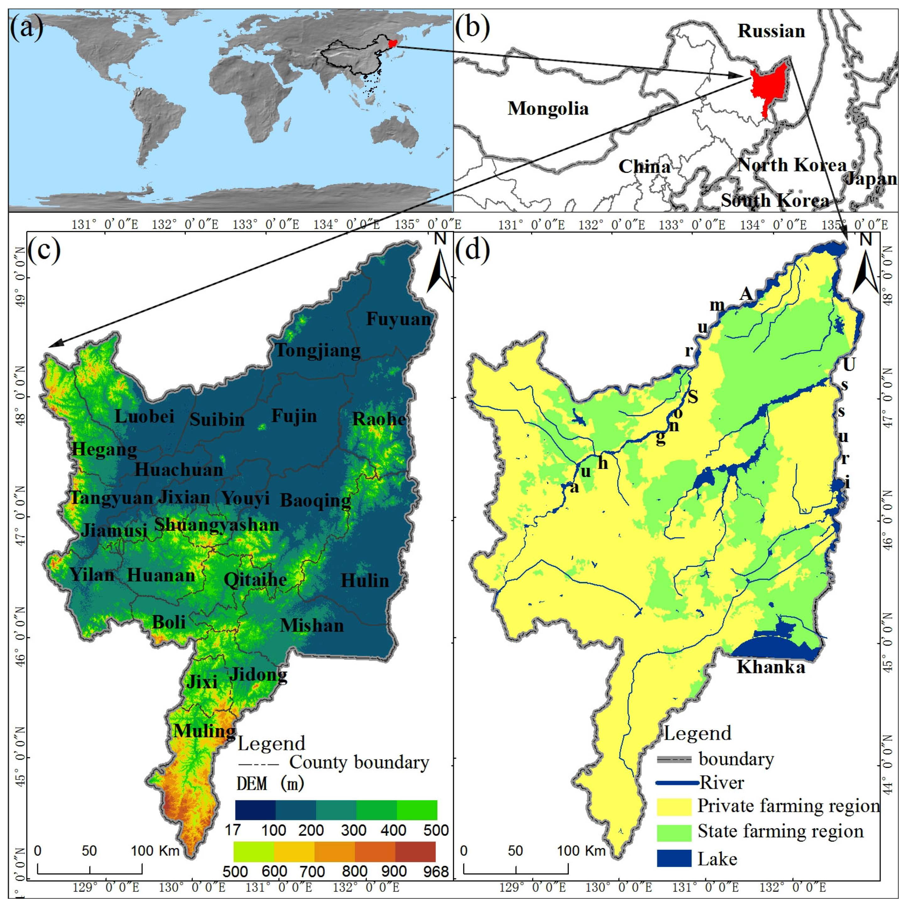
2.1. Study Area

Cold China was defined in the northernmost province of China (43°26′–53°33′N and 121°11′–135°05′E). This region is situated in cold temperate zone, with an annual average temperature below 1 °C. Our study area covers the Sanjiang Plain, which spans the border areas of China and Russia between 45°01′05″–48°27′56″N and 130°13′10″–135°05′26″E (Figure 1a,b) [31], and it covers 23 counties (Figure 1c), with a total area of 10.87 × 10⁴ km2. Of this area, 68.55% (i.e., 7.45 × 10⁴ km2) is assigned to local governments (here, we define it as “private farming”), and the other 31.45% (i.e., 3.42 × 10⁴ km2) is managed by the central government (the definition of “state farming”) (Figure 1d) based on the administrative extent of the state and private farming (the administrative boundaries of the state and private farming were provided from Northeast Agricultural University, China). The Sanjiang Plain (a total of 52 first-level farms) comprises 51.89% (=3.42 × 10⁴ km2) of the state farming area in China (6.61 × 10⁴ km2); thus, this region is critical in the central government’s efforts to adjust the balance between the grain supply and demand in the Chinese agricultural market.
This study area is built upon sediment deposited by the Amur, Ussuri and Songhua rivers (Figure 1d), which provides convenient water conditions for paddy rice planting. The climate is a moderate temperate humid monsoon zone with an annual average temperature of approximately 1 °C–4 °C and an annual average precipitation of 500–650 mm [32]. The black soil is fit for crops with better organic matter. The landform is flat, with elevations ranging from 17 m to 968 m (Figure 1c).

2.2. Data Collection and Analysis

2.2.1. Landsat Image Collection and Preprocessing

The United States Geological Survey (USGS) allows for free data accessibility, which enables the use of all Landsat imagery. Because good-observations for Landsat images in each month were not always available due to the clouds, bad bands, and shadows, it is difficult or impossible to create an annual cropping pattern map through one year’s Landsat images. Thus, it was perhaps to collect the images from many years for crop mapping. We designed the images in an effort to produce an annual map and measured changes in cropping patterns at the time extension ranges of every three years (periods) (1989–1991, 1994–1996, 1999–2001, 2004–2006, 2009–2011, and 2014–2016, Figure 2). All the Landsat TM/ETM + /OLI images (Total number: 4357 scenes, Table 1) from the USGS (https://glovis.usgs.gov/) during these six periods were first visually examined to evaluate the image quality (e.g., clouds, cloud shadows, snow cover, bad strips, etc.). Then, high-quality image observations from the months between April and September were determined based on phenology and crop calendar, which provided good temporal coverage of growing seasons of paddy field and upland crop [33]. A total number of 771 good-observations images (Table 1) for the scenes (paths/rows: 113/27, 114/26, 114/27, 114/28, 114/29, 115/26, 115/27, 115/28, 115/29, 116/27, 116/28, 116/29, Table 2) were downloaded. The Universal Transverse Mercator coordinate system of the images was re-projected to the Albers Conical Equal Area projection to accurately calculate the dynamic area of cropland in this cold region. Meanwhile, radiometric calibration and atmospheric correction were also performed for all the available Landsat images. In order to obtain accurate annual cropping pattern information, we first focused on Landsat images in the special epochs of 1990, 1995, 2000, 2005, 2010, and 2015. If these extracted images failed to cover cropping pattern map for each epoch, the auxiliary extracted images in other epochs were used to fill the blank area where good-observation images were not available in these special epochs. Based on our statistics, 201 extracted images and 38 auxiliary extracted images (Table 1) were used to extract time series cropping pattern information.

2.2.2. Tracking Cropping Information

Paddy field information acquisition. Paddy field has unique property in that it is transplanted in compound surface environments of water and soil. When rice is transplanted, a period of “flood/open-canopy” regularly occurs and is sustained for a few weeks. Other crops, such as wheat, soybean, and corn, do not require transplantation and are not grown in environments with flooded soil. The rice “flood/open-canopy” stage in compound surface environments can be observed with a spectral sensor. After this period, the optical sensors are unable to obtain the water body information below paddy field canopy. Paddy field enters a period of rapid growth and quickly reaches the maturity and harvest phases, from which the spectral characteristics of the paddy field are consistent with those of other crops. Therefore, the best time to remotely extract paddy field data is during the “flood/open-canopy” period, and pixels of from this stage can be identified if the observations meet one of the following conditions: the land surface water index (LSWI, Equation (1) [34]) > the normalized difference vegetation index (NDVI, Equation (2) [35]) or the LSWI > the enhanced vegetation index (EVI, Equation (3) [36]) [37,38], otherwise, the pixels are not identifiable. Multitemporal paddy planting information was acquired through supervised classification in this stage, because the training sites of this stage in Landsat images displayed obvious symbols of paddy field in terms of the hue (dark blue) and regular size. In addition, flooded natural wetland and water body were removed to improve the accuracy. If this step provided insufficient data to meet the annual cartographic needs, auxiliary Landsat images adjacent to the “flood/open-canopy” stage were used through extraction and artificial visual correction.
LSWI = ( ρ g r e e n ρ SWIR ) / ( ρ g r e e n + ρ SWIR )
NDVI = ( ρ N I R ρ r e d ) / ( ρ N I R + ρ r e d )
EVI = 2.5 × ρ N I R ρ r e d ρ N I R + 6 × ρ r e d 7.5 × ρ b l u e + 1
NDWI = ( ρ green - ρ N I R ) / ( ρ g r e e n + ρ N I R )
Excluding flooded natural wetland. Paddy field is also called artificial wetland because it is characterized as both wetland and cropland. Thus, differentiating these land cover types after the rice “flood/open-transplanting” stage using an optical sensor is difficult. Natural wetland is always flooded in late spring due to land surface snowmelt, and the natural wetland grows quickly and reaches NDVI values greater than 0.3 before the period of crop planting [39]. We set a threshold of 0.32 to exclude natural wetland in this “flood/open-transplanting” stage using the matching Landsat images.
Multitemporal water body masks. Multiple masks of water bodies were generated to reduce the error associated with cropping pattern maps, particularly for paddy field, due to the similar spectral signatures in the “flood/open-canopy” stage. Remotely extracted water bodies were chosen from August to September based on multiple Landsat images between 1990 and 2015 in 5-year intervals (1990, 1995, 2000, 2005, 2010, and 2015). During these months, crops entered rapid growth and mature stages, and the sensors cannot monitor water information under the canopy in crops. Normalized Difference Water Index (NDWI, Equation (4) [40]) was performed to achieve spatial water information and the threshold was set to be greater than zero.
Upland crop information acquisition. Upland crop information was obtained from the NLCD dataset in five-year increments from 1990 to 2015. The cropland classification was highly accurate [25], while it does not necessarily support the accuracy of upland crop classification. In this research, we assessed the quality of the multitemporal upland crop data by overlaying it with a corresponding 30-m false-color map (R/G/B = NIR/Red/Green) derived from Landsat TM/ETM + /OLI images. A visual inspection was conducted on all images to correct the misinformation using professional knowledge. Because the classification accuracy of visual interpretation and digitalization images was dependent on the professional knowledge of these individuals. Thus, quality control was implemented via repeated interpretations. In this step, 20% of the dynamic vector polygons in each epoch were randomly selected and reinterpreted to check the quality.
Time series cropping pattern excluding tiny surface features. The new time series cropping pattern (paddy field and upland crop) dataset was created through the NLCD dataset and 266 Landsat images over time. The images were processed based on poor-quality observation detection, image co-registration, atmospheric correction, information extraction, information correction, and data subsetting and stacking (Figure 2). The final product was still a 30-m spatial resolution mixed dataset that embedded the tiny surface features of the cropland areas. The multitemporal and large-scale tiny surface features of the cropland, such as canals, ridges, country roads, tree belts, and construction land for hydraulic engineering, were very difficult to achieve due to the large associated workload and restricted historical high-precision images. In this research, tiny surface features of the cropland obtained through the platform of the Chinese Academy of Sciences and local scientific institutions were used to precisely quantify the cropland map for 2015. The resulting map was combined with the extracted dynamic vector polygons of cropland from the new dataset in each period to refine the status maps of cropland in 2010, 2005, 2000, 1995, and 1990. The new cropping pattern maps were then used to analyze the historical cropland changes under different agricultural systems.

2.2.3. Accuracy Assessment

Accuracy evaluation of new dataset was based on the randomly select samples (pixels), and a number of 400 samples were randomly allocated in the whole study area in each epoch (1990, 1995, 2000, 2005, 2010, and 2015). First, because the areas among different land-use types changed in different epochs, it was better to use the stratified random sampling to select samples in each land use type (e.g., paddy field, upland crop, and other types) in each epoch. Second, for epochs of 1990 and 1995, the samples were referred by the color composite images from Landsat TM due to the difficulty in obtaining good quality and high-resolution images before the year of 2000. The color composites (R/G/B = Bands 5/4/3) in Landsat images displayed obvious symbols of paddy field in terms of the hue (dark blue) and regular size, and the upland crop areas could be identified by their uniform texture (Figure 3a–h). The verified Landsat images were separated from the images that was used to obtain time series cropping pattern information, that means, we used some images (the extracted images and auxiliary extracted images, total number: 239 scenes, Table 1) to obtain cropping pattern information and employed other images (the verified images and auxiliary verified images, total number: 27 scenes, Table 1) to conduct accuracy verification. When an auxiliary extracted image was used, the auxiliary verified image in the same location and same year was also used. The verified images and auxiliary verified images could completely cover the study area and provided all the available samples. Thus, we collected 800 samples for the epochs of 1990 and 1995. Third, for the epochs of 2000, 2005, 2010, and 2015, we obtained the historical imagery archive of Google Earth for these four epochs through the professional authorized payment software (software name: 91 bitmap assistant, website: http://www.91weitu.com/). In order to guarantee the temporal consistency between Landsat source data and validation imagery, we filtered the same years of Google Earth imagery with that of Landsat images used for classification. Specifically, the time of Google images focused on the growing seasons of paddy field and upland crop in the special epochs of 2000, 2005, 2010, and 2015. Based on the boundary in research area, all Google images were downloaded in these four special epochs (resolution: 2 m, date: from April 1st to September 30th in each epoch, sensor: QuickBird, vendor: DigitalGlobe & Google). Based on the stratified random sampling for 400 samples in each epoch, we assigned true/faults for each sample and obtained 217 samples, 266 samples, 347 samples, and 382 samples, because other random samples were unavailable due to the spatial inconsistency in Google Earth images. Meanwhile, we conducted field surveys and marked survey information on the maps, accompanied by confirmed photographs (such as: Figure 3e–h) in the spring and autumn of 2015. There were 3139 field photos collected during field investigation, and these photos provided auxiliary information for accuracy evaluation. Finally, for the land system in the accuracy evaluation, the land classification system of the created dataset in the study was the same with that of the NLCD. In this classification system, all land use types were divided into six first class types, which included cropland, woodland, grassland, water body, construction land, and unused land, and cropland was divided into two categories representing paddy field and upland crop. Then, these verified land types were merged into three types (paddy field, upland crop, and noncropland) based on the needs of this study, and the non-cropland contained five first class types (Figure 3i–l).

2.2.4. Trajectory Transformations

A clustering analysis of the land-use types was conducted for the trajectory transformations. These trajectory transformations include continuous paddy field, continuous upland crop, reclaimed paddy field, reclaimed upland crop, paddy field to upland crop, upland crop to paddy field, paddy field to noncropland, and upland crop to noncropland. The discrimination abilities of the trajectory transformations in the five-year increments (1990–1995, 1995–2000, 2000–2005, 2005–2010, and 2010–2015) were quantified through the land-use confusion matrix approach method. Information on the detailed trajectory transformations for different land use categories can be described in Table 3.

2.2.5. Cropping Pattern Prediction

The Cellular Automata/Markov Change prediction model (CA_MARKOV) is a combined Cellular Automata, Markov Chain, Multi-Criteria, and Multi-Objective Land Allocation land cover prediction system [41]. CA_MARKOV allocates land based on the suitability of the land for end covers along with a cellular automaton rule to promote spatial contiguity. It works well when historical land cover data is not available or is not a good predictor of future land cover [42,43]. Thus, we used CA_MARKOV to extrapolate the cropping patterns for the epochs of 2020, 2030, 2040, and 2050, and further provided some information that CA_MARKOV was well used in the satellite remote sensing analysis domain. In CA_MARKOV, the Markov chain-predicted transitions are usually generated based on only two training land use maps. This approach may provide an inadequate number of training samples. We applied the LUCC budget technique [44,45] to obtain the land changes and the associated component changes, including the total change, gain, loss, and transition, according to the historical land use maps. These training maps were used to determine the Markov chain transition matrices through equal weight coefficients. Based on the Markov chain transition matrices, the Markovian Transition Estimator was used to obtain suitability images for each of the land cover types. In this process, the multiple influencing factor maps in the study area, including the natural factors (streams, slopes, and dem) and socio-economic factors (urban areas, towns, roads, and railways), were added to rectify suitability images, and the Multi-criteria Evaluation (MCE) was conducted to further regulate spatial distribution of suitability images through the thematic maps, including water distribution, ecological protection areas, natural reserves, and land use planning schemes in the study area. Based on the suitability images, the issues with concurrent transitions were solved through the combination of multi-objective land allocation (MOLA) and cellular automata (CA). Then, the predicted maps can be created. In order to test the accuracy of this method in the study area, we utilized the 1990–2010 dataset to predict the map of 2015 (comparison data) and compared it against the real map of 2015 (reference data) in our new dataset (Figure 4). The verification was conducted in the terrset geospatial monitoring and modeling system, and the accuracy verification indicators included quantitative consistency (Kappa location (Klocation)) and spatial consistency (Kappa standard (Kstandard)). The result exhibited high accuracy (Klocation: 0.9714; Kstandard: 0.9302) in the test involving the whole study area. Thus, the method was suitable for land use prediction in this region. We used the method to obtain the suitability images of each land cover type in each epoch (Figure 5) and extrapolated the land prediction maps for the epochs of 2020, 2030, 2040, and 2050.

3. Results

3.1. Validation Accuracy of the New Cropping Pattern Maps

Accuracy assessments of time series of cropping pattern maps were conducted based on the randomly select samples (pixels). The results for the cropland, including paddy field and upland crop, and noncropland maps were highly accurate (Table 4). The overall accuracies were 89.50%, 91.25%, 90.78%, 91.78%, 92.22%, and 93.98% in the different epochs, with corresponding kappa coefficients of 0.87, 0.88, 0.86, 0.88, 0.88, and 0.89, respectively. This finding indicated that the final epoch had the highest overall accuracy and kappa coefficient because of the improved Landsat image intensity and the availability of high-quality Google Earth. The paddy field displayed higher producer accuracy (PA) and user accuracy (UA) in 2015 (PA, 94.44%; UA, 95.03%). The year 1990 exhibited the lowest PA (91.75%) and UA (89.00%), and this result was attributable to the limited intensity of Landsat data. The precision of upland crop classification was similar with that of the paddy field. The time series maps of cropland had high accuracies and could be used for mapping cropping patterns.

3.2. Comparison of the Cropping Patterns between NLCD-Based and New-Based Datasets

Time series maps of cropland in six epochs were generated using a new dataset (Figure 6(a2)–(f2)). The cropland planting area constantly increased from 1990 to 2015, with a total cropland area of 41,167.26 km2 in the first year and 52,507.57 km2 in the final year. During this period, both the NLCD maps (Figure 6(a1)–(g1)) and new dataset (Figure 6(a2)–(g2)) exhibited a continuous and consistent increasing trend for cropland area, despite the differences in the cropping pattern in each epoch. Based on the new dataset, most of cropland area in this region was located on flat plains, with low-lying landscapes and high proportions of swamps, rivers and ditches. Suitable cropland area was generally already cultivated, and further land reclamation was and will continue to be limited (Figure 1d and Figure 6).
The paddy field expanded persistently from the study period. Based on the new dataset, in the first year, paddy field covered very limited areas (2850.87 km2 in total). In these areas, the spatial distribution of paddy field showed in a scattered manner to Songhua River and valley plain along the Khanka. After 1990, the paddy planting area acutely increased and reached 26,537.14 km2 by the final year. The area covered by paddy field in 2015 was 9.3 times greater than that in 1990. During this period, paddy field area reached 4691.24 km2, 9539.90 km2, 12,586.86 km2, and 18,866.99 km2 in epochs of 1995, 2000, 2005, and 2010, respectively (Figure 6(g2)). Paddy expansion first occurred in the western part of the plain along the Songhua river (Figure 6(a2)) and then rapidly increased along the Songhua, Amur, Ussuri and Khanka rivers, where the water resources were abundant near the tributaries and streams of these rivers (Figure 6(b2)–(f2)). Therefore, paddy expansion was mainly based on the accessibility of water resources. Both the NLCD maps and new dataset displayed a continuous increasing trend for the paddy field area in six epochs, while the paddy expansion patterns exhibited apparent inconsistency in each period in both datasets (Figure 6(a1) vs. Figure 6(a2); Figure 6(b1) vs. Figure 6(b2); Figure 6(c1) vs. Figure 6(c2); Figure 6(d1) vs. Figure 6(d2); Figure 6(e1) vs. Figure 6(e2); and Figure 6(f1) vs. Figure 6(f2)). The new dataset had better spatial pattern information for upland crop and paddy field.

3.3. Different Cropping Patterns in Different Agricultural Systems

The area and the percentage of cropland were used to compare different changes under different agricultural systems. The area changes were calculated based on the area in latter epoch subtracted the area in previous epoch, and the percentage were obtained based on the total croplands occupied by paddy field or by upland crop in each epoch in state farming or private farming. The net cropland expansion area on state farming (+6709.64 km2) was faster than that in private farming (+4630.68 km2) during the period of 1990–2015, (Figure 7a,b). Meanwhile, the cropping pattern differed significantly in both regions over time. In private farming (Figure 7a), the percentage of upland crop decreased from 89.88 to 65.02%, with a loss of area of 2840.29 km2, and the percentage of paddy field increased from 10.12 to 34.98%. Thus, the area covered by paddy field increased by 7470.96 km2. While in state farming (Figure 7b), the changes of cropping patterns (including upland crop and paddy field) in state farming changed more rapidly than that in private farming, with the percentage of upland crop obviously decreased from 97.34 to 31.44%, which led to a large loss of area of 9505.66 km2; moreover, the paddy area, as well as the corresponding percentage of total cropland, linearly increased from 467.99 km2 (2.66%) to 16,683.30 km2 (68.56%), thus reflecting an increase of 16,215.30 km2.

3.4. Trajectory Transformations of Cropping Pattern at the Pixel Level in Different Agricultural Systems

Maps of trajectory transformations of cropping patterns, as well as the cropping pattern and noncropland times, were generated based on the new data from all epochs in the study area (Figure 8a,b). For paddy field, the paddy field maps displayed a successive and steadily increasing pattern at the pixel level (Figure 8a). Increase in paddy area was mainly attributable to the transformation of upland crop, which accounted for 83.47%, 90.31%, 85.22%, 76.77% and 73.38% of the reclaimed paddy field in five periods (Table 5). The areas of abandoned paddy field, including the transformation of paddy field to upland crop and paddy field to noncropland, were limited. For upland crop, the trajectory transformation of continuous upland crop was variable at the pixel level (Figure 8b). Increase in upland crop area was mainly due to the transformation of noncropland. This transformation accounted for 98.70%, 98.66%, 99.68%, 96.57% and 89.60% of reclaimed upland crop in five periods. Moreover, areas of abandoned upland crop were converted to paddy field on a large scale. For noncropland, the areas of abandoned cropland converted to paddy field had an increasing trend, with areas of 314 km2, 474 km2, 453 km2, 1468 km2, and 2045 km2 in each period (Table 5). While the opposite trend can be observed in the conversion of abandoned cropland converted to upland crop, with areas of 4238 km2, 2493 km2, 1371 km2, 932 km2, and 114 km2 in each period.
Trajectory transformations of continuous paddy field was inconsistent under different agricultural systems (Figure 8c). In 1990, most paddy field displayed an aggregate distribution in private farming close to the Songhua river and the valley plain (Figure 8(a2)). Additionally, there was very little distribution of crop fields that had paddy field in state farming. Then, on state-run farms, paddy field have acutely expanded to neighboring crops since the year of 2000 (Figure 6 and Figure 8a). So, most paddy field had cropland ages of no more than twenty years following continuous cultivation during 1990–2015 (Figure 8(c3)–(c5)). This situation was also demonstrated in time series cropland maps among six epochs (Figure 6(a2)–(f2)). While in private farming, the reclaimed paddy field lagged behind than that of state-run farming (Figure 8c), although most of the paddy fields were first cultivated more than 25 years before and have been continuous cultivated. A common feature of trajectory transformations of continuous paddy field under different agricultural systems is that paddy transformations presented a northward migration, such as in the directions of c1→c2 for private farming and c3→c4→c5 for state farming, due to the climate warming, increased food demand, and better economic profit for paddy field.

3.5. Cropping Patterns for the Period of 2020–2050

The cropping pattern maps of 2020, 2030, 2040, and 2050 were created based on the prediction (Figure 9a–d). Cropland planting area in this region was predicted to increase by 2602.80 km2 over the thirty-five years, with net changes of +1224.68 km2, +839.57 km2, +565.10 km2, −26.55 km2 in 2015–2020, 2020–2030, 2030–2040 and 2040–2050, respectively. The cropland reclamation area in the future period is much smaller than that in the past period (1990–2015, with a total increase of 11,340.31 km2). It can be noted that cropland growth from 2015 to 2020 accounted for nearly half (47.05%) of the predicted net change. Thus, rapid cropland reclamation is expected to stagnate after the epoch of 2020 due to terrain and spatial land use planning restrictions, such as areas of ecological protection and natural reserves. The paddy planting area is predicted to expand continuously by 7361.25 km2, 9852.57 km2, 3932.54 km2, and 781.15 km2 in each period (Figure 9e–h). This result indicates that rapid paddy expansion become slowness in 2040. Future paddy expansion pattern is first observed in the flat areas neighboring the continuous paddy field along the Songhua, Amur, Ussuri and Khanka Rivers and then extend to several tributaries of these rivers and other areas.
From the perspective of agricultural systems, incremental areas covered by paddy field are still faster in state farming in the period of 2015–2020, while the opposite phenomenon is observed in private farming after that period. In contrast, the areas covered by upland crop will continuously decrease by 6136.57 km2, 9013.00 km2, 3367.44 km2, and 807.70 km2 in each period, with a similar trend in both land ownership regions. Moreover, greater losses of upland crop will occur in private farming that in state farming beginning in 2020.

4. Discussion

4.1. First Region for Continuous and Large-Scale Land Use Transformations from Upland Crop to Paddy Field in China

This study first reported the dynamic tracing of cropping patterns and showed the reasons for paddy expansion in a region of northern Asia. We found that cropping patterns have changed significantly, and continuous rice paddy expansion has occurred, and the land source for paddy expansion was mainly attributed to the large-scale transformations of upland crop. Although a considerable number of paddy fields are located in northern Asia such as northern Japan, northwestern Korea, and China, while dynamic tracking of paddy expansion has not been performed and the source has not been identified in northern Asia. Therefore, we first provide new satellite evidence for these issues in the study area of Cold China. This study showed that continuous and large-scale land use transformations from upland crop to paddy field occurred throughout Cold China, and it represent a new and acute process of land use change in China based on our national survey. At present, China has a large population and limited cropland area [46]. Given the rapid speed of industrialization, urbanization and rural development in the 21st century, the total cropland area in China has decreased [47,48]. This cropland evolution pattern has been characterized by a substantial loss of cropland areas and a reduction in the cropping intensity (such as the cropping intensity from triple cropping to double cropping; and from double cropping to single cropping) in South China, or a return to forest and grassland via ecological restoration projects in Central China. Conversely, the cropping area of single crops has continuously increased in North China, especially in Cold China. Thus, cropland expansion (net change area of +11,340.31 km2 in 1990–2015, Figure 6) in the study area has played an essential role in the maintenance of cropland area in China.
This study showed that cropping patterns in Cold China have varied over time. That is, the area of upland crop shrunk following a large increase, and the area of paddy field continuously expanded during the period of 1990–2015 (Figure 6). This region has been characterized by the rapid expansion of agricultural land, particularly paddy field (net change of +23,686.27 km2 from 1990 to 2015). Therefore, the Cold China has gradually become an important planting base for paddy field in China. Currently, suitable cropping areas are generally already cultivated in areas of low-lying terrain. Further land reclamation will be very limited. Therefore, the cropping pattern displays a new land use phenomenon in which large areas of upland crop are converted to paddy field (Figure 8). This phenomenon first occurred in Cold China due to the large number of state-run farms and appropriate natural resources, such as dense rivers, black soil, and flat terrain. Paddy development in Cold China will continue to guide cropping pattern reformation (Figure 9) in China because this region includes more than half of the state-owned farm areas, which is conducive to the role of the state in adjusting the crop structure in the agricultural market. Meanwhile, paddy field provide a major dietary staple [49] for over 1.3 billion Chinese people and for more than half of the global population.

4.2. Reasons for Different Paddy Patterns under Different Agricultural Systems in China

Agricultural systems are based on two different models in China, and the results presented here indicate that paddy field have expanded at a faster rate and more regularly in state farming than in private farming (Figure 7 and Figure 9). The considerable differences in cropping patterns in both regions can be summarized based on the following factors. (1) Land management regimes. All cropland on state farming is state-owned, and the central government generates annual detailed crop planting plans to adjust the balance in the national agricultural market. According to state regulations, farm governors own land rights and devolve the rights to workers. These workers manage cropland planting, such as paddy field planting in a specific region, under the guidance of the central government and farm governors. While the cropland in private farming is collective-owned and implemented by farmers. Farmers can freely decide the crop planting types and control the land use, management, and benefit right strategies; (2) Agricultural policy. The purpose of agricultural policy has changed over time in China. The goal of the first stage was to provide the basic food for over 1.3 billion Chinese people, and these policies were to promote cropland areas. The “Food First” policy in the First Five-Year Plan (1953–1957) [50] increased the land reclamation area. The “Agricultural Modernization” policy (1978–1985) [51,52] promoted advanced agricultural machinery, and many modernized farms were formed. In the second stage, the goal was to improve people’s agricultural living standard. Although subsequent agricultural policies, such as “Layout Planning for the Advantageous Regions of Rice (2008–2015),” “Sanjiang Plain Land Renovation Project (since 2008)” and “Building High-Standard Basic Farmland”, also generated large-scale cropland reclamation in Cold China; however, these policies focused on cropland quality and cropping patterns (mainly for paddy field). A total of 80–90% of these projects were located in state farming, which effectively improved the agricultural infrastructure and transformed scattered paddy field into an aggregated pattern. Whereas the paddy pattern is scattered in private farming due to the lack of necessary engineering facilities; (3) Restricted water resources and cropland area. Water resources are an important limiting factor for paddy field planting. In state farming, advanced irrigation technology and excellent water facilities provide sufficient water environment for rice planting. Paddy expansion exhibits a “push-and-pull” pattern under surface canal irrigation. However, due to insufficient surface irrigation facilities, paddy expansion in private farming occurs primarily due to the spontaneous drilling of growers, leading to a small-scale and sporadic pattern. Another restricting factor is the cropland area. In state farming, which is characterized by abundant cropland areas and scarce populations, workers obtain cropland via paid annual contracts from farm governors, and they can purchase more land as desired. Notably, paddy field can easily be planted on a large scale (approximately 30–40 hectares/household). However, in private farming, which is characterized by a limited cropland area and a large population, farmers obtain cropland via a 30-year free paid contract, and obtaining more cropland is difficult or impossible. Moreover, a paddy field in private farming can only be planted on a small scale (approximately 2–6 hectares/household) based on our survey.

4.3. Driving of Physical Conditions and Human Factors on New Cropping Pattern Changes in Cold and High Latitudes of China

The driving forces underlying the new land use changes can be summarized based on two aspects. The first aspect is the physical conditions, such as water resources, soil resources, and topography. Paddy expansion is mainly based on the accessibility of water resources. The region is built upon sediment deposited by the Amur, Ussuri and Songhua rivers, which provides convenient water conditions for paddy rice planting. This region is one of the three black soil regions on Earth, and the black soil is more fit for rice planting because of its good organic matter content and high fertility. The terrain is flat, which is propitious to water storage in paddy patches. The second aspect is human factors, such as agricultural policy, agricultural technological progress, and crop economic returns. This region covers more than half of the cropland area of state-run farms in China, and many agricultural policies and water conservancy projects are focused on state farming regions, which improves the infrastructure in paddy field. Agricultural technological progress increases the adaptability of seeds and the efficiency of fertilization in cold regions; and thus, promotes rice paddy expansion. The economic returns that the net income of paddy field (average more than 8500 yuan/hm2) is higher than that of upland crop (average less than 6500 yuan/hm2) is another human factor underlying paddy expansion in cold regions.

4.4. Effect of Cropping Pattern Changes on the Environment in Cold Region

Cold China is a commodity grain production base in China and was covered by a large area of upland crop in 1990. Continuous and acute land use change from upland crop (mainly soybean) to paddy field will inevitably affect the terrestrial carbon cycle and lead to the large-scale loss of carbon dioxide in this cold region [53,54,55,56]. Additionally, paddy expansion influences the surface energy balance and greenhouse gas emissions in addition to virus transmission due to its characteristics as both wetland and cropland. Paddy field planting obviously reduces the surface temperature and changes the Bowen ratio during the growing season; and it is also a significant source of methane flux into the atmosphere and contributes more than ten percent of worldwide methane emissions. As a vital habitat for wild animals, such as free-ranging ducks and waterfowl species, paddy field is related to the spread of avian influenza viruses and other diseases. By growing in a flooded soil environment, paddy expansion may have the most apparent influence on water resource utilization. Rapid and acute paddy expansion in Cold China accelerated river water irrigation and groundwater overexploitation, and such change may increase the risk of groundwater depletion to a certain extent. Based on the study, the paddy expansion will continue in Cold China after 2020, especially in private farming region. In these regions, surface water resources are not abundant compared to those in state farming. A comprehensive evaluation of the carrying capacity of agricultural water resources is needed to provide an early scientific warning and coordinate the water resources and paddy planting area in cold regions. Meanwhile, with the exception of environmental issues involving the changes in paddy field expansion and upland crop shrinkage, the issues caused by the loss of noncropland should not be ignored. The expansion in cropland was mainly at the loss of woodland, grassland and unused land in noncropland based on our survey. Thus, these issues were multiple fields, such as the loss in carbon source/sink in woodland and the loss of biodiversity in unused land in ecology, and the changes in air temperature and evapotranspiration among different land use types in climatology.

4.5. Uncertainty of Crop Information Extraction and Future Prediction

The main uncertainties in this research was related to two factors. (1) The availability of good-observations in Landsat images. The accuracy of land use information acquisition depends on the quality of remote sensing images. Good-observations in Landsat images can comprehensively and accurately track dynamic information. Therefore, the cropping pattern based on remote sensing information during 1989–2016 is mainly limited by image quality in this research. Specifically, the rice “flood/open-canopy” stage is short. With restricted number of images per year (accompanied by 16-day revisit cycle with Landsat data) and uncertain image quality (clouds, bad strips, etc.), establishing an annual cropping pattern map via the Landsat images for one year is difficult or impossible. Thus, this research designed images to create an annual map and measured the changes in cropping pattern in the time resolution over three years. If the data in stage of rice” flood/open-canopy” failed to meet the cartographic requirements in the special epochs of 1990, 1995, 2000, 2005, 2010, and 2015, we extended the data time throughout the growing season in these special epochs. If the maps still failed to cover the whole study in each epoch, the auxiliary Landsat images adjacent to special epochs were used to fill the blank area where good-observation images were not available in these special epochs. Finally, 222 images in special epochs and 44 images in other epochs (Table 1) were used to finish time series cropping pattern mapping; (2) The uncertainty for cropping pattern prediction. Based on the past changes of cropping pattern areas, a potential and reliable future development scenario was given in this study. To reduce the uncertainty of land prediction, we used the LUCC budget technique to obtain the relations between the nonstationary processes and predictability needs based on Markov chain transition matrices through various training maps in each period. Moreover, the natural factors, social and economic factors, and thematic maps were added to accurately predict the suitability images of each land cover type in each epoch. In this scenario, the information regarding paddy field planning and water consumption was not included due to the sufficient water resources (total storage: 202.31 × 10⁸ m3; annual average precipitation: 567.50 × 10⁸ m3; annual average flow: 2634.26 × 108 m3) in the study area. Given the apparent influence of paddy expansion on water resource utilization, the assessments of paddy field planting areas and available water resources are needed in future research. Meanwhile, the shortcoming in future prediction is that this study didn’t take into account the impacts of possible changes in climate and food consumption preferences on cropping patterns in the future, such as the new crop that will fit better for this region climate and will increase the growers’ profit in Cold China. These new crops (the exclusion of paddy field) also have the possibility to expand in the future. Because the changes in cropland are often nonlinear (e.g., progressive or regressive, slow or fast), and cropland often displays a high degree of space-time complexity and complicated feedback mechanisms [57,58,59]. However, due to the complexity of changes in land use, climate, and human activity, it is difficult to make reliable multi-scenario prediction at present. These issues will be our important research directions in the future. We’ll report them immediately as soon as we get any signals of the new crops.

5. Conclusions

Large-scale applications of time series Landsat images in cropland change studies beginning in 1990 face various challenges, such as variable image quality (e.g., clouds and bad strips) and inhomogeneous data availability at spatial and temporal scales. Based on time series of Landsat images, this study attempts to track cropping information (1990–2015) and predicts the future pattern (2015–2050) under different agricultural systems in Cold China by developing an updated method for determining cropland patterns. The results demonstrated that the available Landsat images in Cold China met the requirements for long-term cropping pattern studies; and the developed method exhibited high accuracy and good spatial pattern results. Based on the new cropping pattern dataset, the cropping pattern significantly differed in both agricultural systems, with paddy field in state farming expanding at a faster rate (from 2.66 to 68.56%) than those in private farming (from 10.12 to 34.98%). Paddy expansion was mainly attributable to the transformation of upland crop at the pixel level, which led to a greater loss of upland crops in state farming than private farming (9505.66 km2 vs. 2840.29 km2) from 1990 to 2015. Meanwhile, the loss in non-cropland was first mainly converted to upland crop and then primarily converted to paddy field. Based on the prediction, rapid cropland reclamation will be projected to stagnate in 2020, while paddy expansion will continue until 2040 primarily in private farming areas in Cold China. This study provides new satellite evidence showing that different agricultural systems significantly affected cropping patterns through rice paddy expansion, and the results have significant implications for understanding and guiding agroecosystem development.

Author Contributions

Conceptualization, Wenhui Kuang; Data curation, Chi Zhang; Methodology, Tao Pan; Visualization, Chi Zhang; Writing—original draft, Tao Pan; Writing—review & editing, Chi Zhang, Wenhui Kuang, Philippe De Maeyer, Alishir Kurban, Rafiq Hamdi and Guoming Du.

Funding

This research was funded by the Strategic Priority Research Program of Chinese Academy of Sciences, Grant No. XDA2006030201 and Chi Zhang is supported by the Taishan Scholars Program of Shandong, China, Grant No. ts201712071; Guoming Du is supported by the National Natural Science Foundation of China (41571167).

Conflicts of Interest

The authors declare no conflicts of interest. The founding sponsors had no role in the design of the study; in the collection, analyses, or interpretation of the data; in the writing of the manuscript, and in the decision to publish the results.

References

  1. Liu, J.; Kuang, W.; Zhang, Z.; Xu, X.; Qin, Y.; Ning, J.; Zhou, W.; Zhang, S.; Li, R.; Yan, C. Spatiotemporal characteristics, patterns, and causes of land-use changes in China since the late 1980s. J. Geogr. Sci. 2014, 24, 195–210. [Google Scholar] [CrossRef]
  2. Lambin, E.F.; Geist, H.J. Land-Use and Land-Cover Change: Local Processes and Global Impacts; Springer Science & Business Media: New York, NY, USA, 2008. [Google Scholar]
  3. Meroni, M.; Schucknecht, A.; Fasbender, D.; Rembold, F.; Fava, F.; Mauclaire, M.; Goffner, D.; Di Lucchio, L.M.; Leonardi, U. Remote sensing monitoring of land restoration interventions in semi-arid environments with a before–after control-impact statistical design. Int. J. Appl. Earth Obs. Geoinf. 2017, 59, 42–52. [Google Scholar] [CrossRef] [PubMed]
  4. Popp, J.; Lakner, Z.; Harangi-Rakos, M.; Fari, M. The effect of bioenergy expansion: Food, energy, and environment. Renew. Sustain. Energy Rev. 2014, 32, 559–578. [Google Scholar] [CrossRef]
  5. Thenkabail, P.S.; Dheeravath, V.; Biradar, C.M.; Gangalakunta, O.R.P.; Noojipady, P.; Gurappa, C.; Velpuri, M.; Gumma, M.; Li, Y. Irrigated area maps and statistics of India using remote sensing and national statistics. Remote Sens. 2009, 1, 50–67. [Google Scholar] [CrossRef]
  6. Tian, H.; Ren, W.; Tao, B.; Sun, G.; Chappelka, A.; Wang, X.; Pan, S.; Yang, J.; Liu, J.; Felzer, B.S. Climate extremes and ozone pollution: A growing threat to China’s food security. Ecosyst. Health Sustain. 2016, 2, e01203. [Google Scholar] [CrossRef]
  7. Liu, J.; Liu, M.; Tian, H.; Zhuang, D.; Zhang, Z.; Zhang, W.; Tang, X.; Deng, X. Spatial and temporal patterns of China’s cropland during 1990–2000: An analysis based on Landsat TM data. Remote Sens. Environ. 2005, 98, 442–456. [Google Scholar] [CrossRef]
  8. Xiubin, L. A review of the international researches on land use/land cover change. Acta Geogr. Sin. 1996, 6, 553–558. [Google Scholar]
  9. Kuang, W.; Liu, J.; Dong, J.; Chi, W.; Zhang, C. The rapid and massive urban and industrial land expansions in China between 1990 and 2010: A CLUD-based analysis of their trajectories, patterns, and drivers. Landsc. Urban Plan. 2016, 145, 21–33. [Google Scholar] [CrossRef] [Green Version]
  10. Dai, S.; Li, H.; Luo, H.; Zhao, Y.; Zhang, K. Changes of annual accumulated temperature over Southern China during 1960–2011. J. Geogr. Sci. 2015, 25, 1155–1172. [Google Scholar] [CrossRef]
  11. Wang, L.; Song, C.; Song, Y.; Guo, Y.; Wang, X.; Sun, X. Effects of reclamation of natural wetlands to a rice paddy on dissolved carbon dynamics in the Sanjiang Plain, Northeastern China. Ecol. Eng. 2010, 36, 1417–1423. [Google Scholar] [CrossRef]
  12. Shi, W.; Tao, F.; Liu, J.; Xu, X.; Kuang, W.; Dong, J.; Shi, X. Has climate change driven spatio-temporal changes of cropland in northern China since the 1970s? Clim. Chang. 2014, 124, 163–177. [Google Scholar] [CrossRef]
  13. Pielke, R.A. Land use and climate change. Science 2005, 310, 1625–1626. [Google Scholar] [CrossRef] [PubMed]
  14. Zhang, C.; Tian, H.; Chen, G.; Chappelka, A.; Xu, X.; Ren, W.; Hui, D.; Liu, M.; Lu, C.; Pan, S. Impacts of urbanization on carbon balance in terrestrial ecosystems of the Southern United States. Environ. Pollut. 2012, 164, 89–101. [Google Scholar] [CrossRef] [PubMed]
  15. Poeplau, C.; Don, A. Carbon sequestration in agricultural soils via cultivation of cover crops–A meta-analysis. Agric. Ecosyst. Environ. 2015, 200, 33–41. [Google Scholar] [CrossRef]
  16. Kebede, Y.; Baudron, F.; Bianchi, F.; Tittonell, P. Unpacking the push-pull system: Assessing the contribution of companion crops along a gradient of landscape complexity. Agric. Ecosyst. Environ. 2018, 268, 115–123. [Google Scholar] [CrossRef]
  17. Kim, D.-G. Nitrous Oxide and Methane Fluxes in Riparian Buffers and Adjacent Crop Fields; Iowa State University: Ames, IA, USA, 2008. [Google Scholar]
  18. Friedl, M.A.; McIver, D.K.; Hodges, J.C.; Zhang, X.; Muchoney, D.; Strahler, A.H.; Woodcock, C.E.; Gopal, S.; Schneider, A.; Cooper, A. Global land cover mapping from MODIS: Algorithms and early results. Remote Sens. Environ. 2002, 83, 287–302. [Google Scholar] [CrossRef]
  19. Hansen, M.C.; DeFries, R.S.; Townshend, J.R.; Sohlberg, R. Global land cover classification at 1 km spatial resolution using a classification tree approach. Int. J. Remote Sens. 2000, 21, 1331–1364. [Google Scholar] [CrossRef] [Green Version]
  20. Woodcock, C.E.; Allen, R.; Anderson, M.; Belward, A.; Bindschadler, R.; Cohen, W.; Gao, F.; Goward, S.N.; Helder, D.; Helmer, E. Free access to Landsat imagery. Science 2008, 320, 1011. [Google Scholar] [CrossRef]
  21. Liu, J.; Zhang, Z.; Xu, X.; Kuang, W.; Zhou, W.; Zhang, S.; Li, R.; Yan, C.; Yu, D.; Wu, S. Spatial patterns and driving forces of land use change in China during the early 21st century. J. Geogr. Sci. 2010, 20, 483–494. [Google Scholar] [CrossRef]
  22. Chen, L.; Huang, Z.; Gong, J.; Fu, B.; Huang, Y. The effect of land cover/vegetation on soil water dynamic in the hilly area of the loess plateau, China. Catena 2007, 70, 200–208. [Google Scholar] [CrossRef]
  23. Gao, J.; Liu, Y. Determination of land degradation causes in Tongyu County, Northeast China via land cover change detection. Int. J. Appl. Earth Obs. Geoinf. 2010, 12, 9–16. [Google Scholar] [CrossRef]
  24. Zhou, Q.; Li, B.; Kurban, A. Spatial pattern analysis of land cover change trajectories in Tarim Basin, northwest China. Int. J. Remote Sens. 2008, 29, 5495–5509. [Google Scholar] [CrossRef]
  25. Zhang, Z.; Wang, X.; Zhao, X.; Liu, B.; Yi, L.; Zuo, L.; Wen, Q.; Liu, F.; Xu, J.; Hu, S. A 2010 update of National Land Use/Cover Database of China at 1:100000 scale using medium spatial resolution satellite images. Remote Sens. Environ. 2014, 149, 142–154. [Google Scholar] [CrossRef]
  26. Yan, F.; Zhang, S.; Kuang, W.; Du, G.; Chen, J.; Liu, X.; Yu, L.; Yang, C. Comparison of cultivated landscape changes under different management modes: A case study in Sanjiang Plain. Sustainability 2016, 8, 1071. [Google Scholar] [CrossRef]
  27. Lin, G.; Ho, S.P. The state, land system, and land development processes in contemporary China. Ann. Assoc. Am. Geogr. 2005, 95, 411–436. [Google Scholar] [CrossRef]
  28. Ye, Y.; Fang, X. Spatial pattern of land cover changes across Northeast China over the past 300 years. J. Hist. Geogr. 2011, 37, 408–417. [Google Scholar] [CrossRef]
  29. Wang, Z.; Zhang, B.; Zhang, S.; Li, X.; Liu, D.; Song, K.; Li, J.; Li, F.; Duan, H. Changes of land use and of ecosystem service values in Sanjiang Plain, Northeast China. Environ. Monit. Assess. 2006, 112, 69–91. [Google Scholar] [CrossRef]
  30. Ecsedy, C.J.; Murphy, C.G. Global climate warming. Water Environ. Res. 1992, 64, 647–653. [Google Scholar]
  31. Liu, H.; Zhang, S.; Li, Z.; Lu, X.; Yang, Q. Impacts on wetlands of large-scale land-use changes by agricultural development: The small Sanjiang Plain, China. Ambio A J. Hum. Environ. 2004, 33, 306–310. [Google Scholar] [CrossRef]
  32. Song, K.; Liu, D.; Wang, Z.; Zhang, B.; Jin, C.; Li, F.; Liu, H. Land use change in Sanjiang Plain and its driving forces analysis since 1954. Acta Geogr. Sin. 2008, 63, 93. [Google Scholar]
  33. Tao, F.; Zhang, Z.; Zhang, S.; Zhu, Z.; Shi, W. Response of crop yields to climate trends since 1980 in China. Clim. Res. 2012, 54, 233–247. [Google Scholar] [CrossRef]
  34. Chandrasekar, K.; Sesha Sai, M.; Roy, P.; Dwevedi, R. Land Surface Water Index (LSWI) response to rainfall and NDVI using the MODIS Vegetation Index product. Int. J. Remote Sens. 2010, 31, 3987–4005. [Google Scholar] [CrossRef]
  35. Tucker, C.J. Red and photographic infrared linear combinations for monitoring vegetation. Remote Sens. Environ. 1979, 8, 127–150. [Google Scholar] [CrossRef] [Green Version]
  36. Huete, A.; Didan, K.; Miura, T.; Rodriguez, E.P.; Gao, X.; Ferreira, L.G. Overview of the radiometric and biophysical performance of the MODIS vegetation indices. Remote Sens. Environ. 2002, 83, 195–213. [Google Scholar] [CrossRef]
  37. Xiao, X.; Boles, S.; Frolking, S.; Li, C.; Babu, J.Y.; Salas, W.; Moore, B., III. Mapping paddy rice agriculture in South and Southeast Asia using multi-temporal MODIS images. Remote Sens. Environ. 2006, 100, 95–113. [Google Scholar] [CrossRef]
  38. Xiao, X.; Boles, S.; Liu, J.; Zhuang, D.; Frolking, S.; Li, C.; Salas, W.; Moore, B., III. Mapping paddy rice agriculture in southern China using multi-temporal MODIS images. Remote Sens. Environ. 2005, 95, 480–492. [Google Scholar] [CrossRef]
  39. Dong, J.; Xiao, X.; Kou, W.; Qin, Y.; Zhang, G.; Li, L.; Jin, C.; Zhou, Y.; Wang, J.; Biradar, C.; et al. Tracking the dynamics of paddy rice planting area in 1986–2010 through time series Landsat images and phenology-based algorithms. Remote Sens. Environ. 2015, 160, 99–113. [Google Scholar] [CrossRef] [Green Version]
  40. McFeeters, K. The use of the Normalized Difference Water Index (NDWI) in the delineation of open water features. Int. J. Remote Sens. 1996, 17, 1425–1432. [Google Scholar] [CrossRef]
  41. Olmedo, M.T.C.; Paegelow, M.; Mas, J.-F.; Escobar, F. Geomatic Approaches for Modeling Land Change Scenarios; Springer: Berlin/Heidelberg, Germany, 2018. [Google Scholar]
  42. Etemadi, H.; Smoak, J.M.; Karami, J. Land use change assessment in coastal mangrove forests of Iran utilizing satellite imagery and CA–Markov algorithms to monitor and predict future change. Environ. Earth Sci. 2018, 77, 208. [Google Scholar] [CrossRef]
  43. Nadoushan, M.; Soffianian, A.; Alebrahim, A. Modeling land use/cover changes by the combination of Markov chain and cellular automata Markov (CA-Markov) models. J. Earth Environ. Health Sci. 2015, 1, 16. [Google Scholar] [CrossRef]
  44. Pontius, R.G.; Boersma, W.; Castella, J.-C.; Clarke, K.; de Nijs, T.; Dietzel, C.; Duan, Z.; Fotsing, E.; Goldstein, N.; Kok, K. Comparing the input, output, and validation maps for several models of land change. Ann. Reg. Sci. 2008, 42, 11–37. [Google Scholar] [CrossRef]
  45. Pontius, R.G., Jr.; Huffaker, D.; Denman, K. Useful techniques of validation for spatially explicit land-change models. Ecol. Model. 2004, 179, 445–461. [Google Scholar] [CrossRef]
  46. Yang, H.; Li, X. Cultivated land and food supply in China. Land Use Policy 2000, 17, 73–88. [Google Scholar] [CrossRef]
  47. Kuang, W.; Chi, W.; Lu, D.; Dou, Y. A comparative analysis of megacity expansions in China and the US: Patterns, rates and driving forces. Landsc. Urban Plan. 2014, 132, 121–135. [Google Scholar] [CrossRef]
  48. Liu, Y.; Liu, Y.; Chen, Y.; Long, H. The process and driving forces of rural hollowing in China under rapid urbanization. J. Geogr. Sci. 2010, 20, 876–888. [Google Scholar] [CrossRef]
  49. Elert, E. Rice by the numbers: A good grain. Nature 2014, 514, S50. [Google Scholar] [CrossRef]
  50. Wang, Z.; Song, K.; Ma, W.; Ren, C.; Zhang, B.; Liu, D.; Chen, J.M.; Song, C. Loss and fragmentation of marshes in the Sanjiang Plain, Northeast China, 1954–2005. Wetlands 2011, 31, 945. [Google Scholar] [CrossRef]
  51. Huang, J.; Rozelle, S.; Wang, H. Fostering or stripping rural China: Modernizing agriculture and rural to urban capital flows. Dev. Econ. 2006, 44, 1–26. [Google Scholar] [CrossRef]
  52. Liu, X.; Dong, G.; Wang, X.; Xue, Z.; Jiang, M.; Lu, X.; Zhang, Y. Characterizing the spatial pattern of marshlands in the Sanjiang Plain, Northeast China. Ecol. Eng. 2013, 53, 335–342. [Google Scholar] [CrossRef]
  53. Tian, H.; Chen, G.; Lu, C.; Xu, X.; Ren, W.; Zhang, B.; Banger, K.; Tao, B.; Pan, S.; Liu, M. Global methane and nitrous oxide emissions from terrestrial ecosystems due to multiple environmental changes. Ecosyst. Health Sustain. 2015, 1, 1–20. [Google Scholar] [CrossRef] [Green Version]
  54. Xu, X.; Tian, H.; Chen, G.; Liu, M.; Ren, W.; Lu, C.; Zhang, C. Multifactor controls on terrestrial N2O flux over North America from 1979 through 2010. Biogeosciences 2012, 9, 1351. [Google Scholar] [CrossRef]
  55. Zhang, Y.; Wang, Y.; Su, S.; Li, C. Quantifying methane emissions from rice paddies in Northeast China by integrating remote sensing mapping with a biogeochemical model. Biogeosciences 2011, 8, 1225–1235. [Google Scholar] [CrossRef] [Green Version]
  56. Zhang, C.; Tian, H.; Pan, S.; Lockaby, G.; Chappelka, A. Multi-factor controls on terrestrial carbon dynamics in urbanized areas. Biogeosciences 2014, 11, 7107. [Google Scholar] [CrossRef]
  57. Verburg, P.H. Simulating feedbacks in land use and land cover change models. Landsc. Ecol. 2006, 21, 1171–1183. [Google Scholar] [CrossRef]
  58. Chave, J.; Réjou-Méchain, M.; Búrquez, A.; Chidumayo, E.; Colgan, M.S.; Delitti, W.B.; Duque, A.; Eid, T.; Fearnside, P.M.; Goodman, R.C. Improved allometric models to estimate the aboveground biomass of tropical trees. Glob. Chang. Biol. 2014, 20, 3177–3190. [Google Scholar] [CrossRef] [PubMed]
  59. Cartwright, W.; Gartner, G.; Meng, L.; Peterson, M. Lecture Notes in Geoinformation and Cartography; Springer: Berlin/Heidelberg, Germany, 2007. [Google Scholar]
Figure 1. Global and regional scale locations of the study area (a,b); digital elevation model (DEM) and county boundaries (c); and main water bodies and administrative extent of the state and private farming (d).
Remotesensing 10 02011 g001
Figure 2. Flow chart for developing an updated method of determining cropland patterns. The new time series cropping pattern dataset in five-year increments from 1990 to 2015 based on the NLCD dataset and multiple Landsat images, and the predicted future patterns for the period of 2020–2050.
Remotesensing 10 02011 g002
Figure 3. Validation symbols in remote sensing images and field survey photographs. (a,b): 30-m color composite images from Landsat TM; (c,d): cropping pattern (paddy field and upland crop) historical imagery archived by Google Earth; (e,f): survey photographs of paddy field in early June and late June 2015; (g,h): survey photographs of upland crops in early June and mid-June 2015; (il) Non-cropland class; including woodland (i); water body (j); construction land (k); and unused land (l).
Remotesensing 10 02011 g003
Figure 4. (a) Resulted map (comparison data) based on the prediction in 2015; and (b) Real map (reference data) based on the new dataset in 2015.
Remotesensing 10 02011 g004
Figure 5. Suitability images of each land cover type in the epochs of 2020, 2030, 2040, and 2050. (a) 2020; (b) 2030; (c) 2040; and (d) 2050.
Remotesensing 10 02011 g005
Figure 6. Resulting maps of cropping patterns and statistics for the NLCD-based and new-based datasets of the Sanjiang Plain in the six epochs from 1990 to 2015. Cropping patterns: NLCD-based dataset: (a1): 1990; (b1): 1995; (c1): 2000; (d1): 2005; (e1): 2010; and (f1): 2015; new-based dataset: (a2): 1990; (b2): 1995; (c2): 2000; (d2): 2005; (e2): 2010; and (f2): 2015. Statistics: (g1): NLCD-based dataset; (g2): new-based dataset.
Remotesensing 10 02011 g006
Figure 7. The total cropland area and the areas covered by upland crop and by paddy field in the state and private farming are showed in Figure 7(a1,2). The percentage of total croplands occupied by paddy field and by upland crop in the state and private farming are showed in Figure 7(b1,2).
Remotesensing 10 02011 g007
Figure 8. Trajectory transformations of the cropping patterns at the pixel level from 1990 to 2015. (a) Transition dynamics of the paddy field between two epochs. The figure shows a specific region from the black box in (a); (b) Transition dynamics of upland crop between two epochs. The figure shows a specific from the black box in (b); (c) The year (epoch) when a pixel in remote sensing image is identified as the paddy region for the first time. Five boxes were selected to show the trajectory directions of paddy dynamics at the pixel scale over five periods in private farming (two boxes: (c1), (c2)) and state farming (three boxes: (c3), (c4), (c5)).
Remotesensing 10 02011 g008
Figure 9. Resulting maps of the predicted cropping patterns and statistics. The predicted cropping patterns: (a): 2020; (b): 2030; (c): 2040; (d): 2050; statistics: (e,f): percentages of the upland crop and paddy field made up of cropland in private and state farming, (g,h): dynamic area of upland crop and paddy field in each period in private and state farming.
Remotesensing 10 02011 g009
Table 1. Statistical information regarding the Landsat images for time series cropping pattern extraction.
Periods1989–19911994–19961999–20012004–20062009–20112014–2016Total
Total Landsat images7947557476905588134357
Good-observations images135154145113100124771
Epochs199019952000200520102015Total
Extracted images 253354213236201
Auxiliary extracted images 563135638
Verified images 1011--------21
Auxiliary verified images33--------6
Table 2. Statistical information regarding the good-observations Landsat images for the path/row in each period.
1989–19911994–19961999–20012004–20062009–20112014–2016Total
113/0271211141391069
114/0261316141051068
114/0271414101081167
114/028151313761064
114/029131411961265
115/02671214891363
115/02791212712860
115/0281191178753
115/0297111289956
116/0271016111281168
116/02810141310111371
116/0291412101291067
Total135154145113100124771
Table 3. Detailed information regarding the trajectory transformations for different categories.
TypesEpoch 1Epoch 2Epoch 3Epoch 4Epoch 5TypesEpoch 1Epoch 2Epoch 3Epoch 4Epoch 5
c pp0→p1p1→p2p2→p3p3→p4p4→p5c uu0→u1u1→u2u2→u3u3→u4u4→u5
r pnc0→p1nc1→p2nc2→p3nc3→p4nc4→p5r unc0→u1nc1→u2nc2→u3nc3→u4nc4→u5
p→ncp0→ nc1p1→nc2p2→nc3p3→nc4p4→nc5u→ncu0→nc1u1→nc2u2→nc3u3→nc4u4→nc5
p→up0→u1p1→u2p2→u3p3→u4p4→u5u→pu0→p1u1→p2u2→p3u3→p4u4→p5
Notes: p: paddy field; u: upland crop; nc: noncropland; c p: continuous paddy field; r p: reclaimed paddy field; p→nc: paddy field to noncropland; p→u: paddy field to upland crop; c u: continuous upland crop; r p: reclaimed upland crop; u→nc: upland crop to noncropland; u→p: upland crop to paddy field; period i (i = 1, 2, 3, 4, 5) represents the time period stages of 1990–1995, 1995–2000, 2000–2005, 2005–2010, and 2010–2015, respectively.
Table 4. Confusion matrix of land-use validation based on Landsat TM and Google Earth imagery in the special epochs of 1990, 1995, 2000, 2005, 2010, and 2015. The overall accuracy (OA), user accuracy, producer accuracy, and kappa coefficients are also provided.
Ground Truth (GT) Samples (Pixels)Total Classified PixelsUser’s Accuracy
YearLand-Use TypePaddy FieldUpland CropNon-Cropland
1990Paddy field894710089.00%
Upland crop31511016492.07%
Non-cropland51311813686.76%
Total GT pixels97168135400OA = 89.50%
Producer’s Accuracy91.75%89.88%87.41% Kappa = 0.87
1995Paddy field1264713791.97%
Upland crop1112912291.80%
Non-cropland9512714190.07%
Total GT pixels136121143400OA = 91.25%
Producer’s Accuracy92.65%92.56%88.81% Kappa = 0.88
2000Paddy field54246090.00%
Upland crop18148694.19%
Non-cropland36627286.11%
Total GT pixels588969217OA = 90.78%
Producer’s Accuracy93.10%91.01%89.86% Kappa = 0.86
2005Paddy field78248492.86%
Upland crop16957592.00%
Non-cropland649710790.65%
Total GT pixels8575107266OA = 91.78%
Producer’s Accuracy91.76%92.00%91.59% Kappa = 0.88
2010Paddy field1345514493.06%
Upland crop193610093.00%
Non-cropland739310390.29%
Total GT pixels142101104347OA = 92.22%
Producer’s Accuracy94.37%92.08%89.42% Kappa = 0.88
2015Paddy field1533516195.03%
Upland crop3106411393.81%
Non-cropland6210010892.59%
Total GT pixels162111109382OA = 93.98%
Producer’s Accuracy94.44%95.50%91.74% Kappa = 0.89
Table 5. Trajectory transformations of land use for the periods of 1990–1995, 1995–2000, 2000–2005, 2005–2010, and 2010–2015 (km2).
1990–19951995–20002000–20052005–20102010–2015
Croplandc p27854643952212,54418852
p→u553443313
c u35,74835,04534,30930,56325,842
u→p15904421261248535638
Cropland and Noncroplandnc→p31447445314682045
nc→u423824931371932114
p→nc91314105
u→nc97757565126648
Notes: p: paddy field; u: upland crop; nc: noncropland; c p: continuous paddy field; p→nc: paddy field to noncropland; p→u: paddy field to upland crop; c u: continuous upland crop; u→nc: upland crop to noncropland; u→p: upland crop to paddy field.

