Article

Optical Tracking Velocimetry (OTV): Leveraging Optical Flow and Trajectory-Based Filtering for Surface Streamflow Observations

1
Department for Innovation in Biological, Agro-food and Forest Systems, University of Tuscia, 01100 Viterbo, Italy
2
Dipartimento di Informatica—Scienza e Ingegneria, University of Bologna, 40141 Bologna, Italy
3
Dipartimento di Ingegneria Civile, Chimica, Ambientale e dei Materiali, University of Bologna, 40141 Bologna, Italy
4
Department of Mechanical and Aerospace Engineering, Tandon School of Engineering, New York University, Brooklyn, NY 10003, USA
*
Author to whom correspondence should be addressed.
Remote Sens. 2018, 10(12), 2010; https://doi.org/10.3390/rs10122010
Submission received: 25 October 2018 / Revised: 5 December 2018 / Accepted: 9 December 2018 / Published: 11 December 2018
(This article belongs to the Special Issue Remote Sensing of Surface Runoff)

Abstract

:
Nonintrusive image-based methods have the potential to advance hydrological streamflow observations by providing spatially distributed data at high temporal resolution. Due to their simplicity, correlation-based approaches have until recent been preferred to alternative image-based approaches, such as optical flow, for camera-based surface flow velocity estimate. In this work, we introduce a novel optical flow scheme, optical tracking velocimetry (OTV), that entails automated feature detection, tracking through the differential sparse Lucas-Kanade algorithm, and then a posteriori filtering to retain only realistic trajectories that pertain to the transit of actual objects in the field of view. The method requires minimal input on the flow direction and camera orientation. Tested on two image data sets collected in diverse natural conditions, the approach proved suitable for rapid and accurate surface flow velocity estimations. Five different feature detectors were compared and the features from accelerated segment test (FAST) resulted in the best balance between the number of features identified and successfully tracked as well as computational efficiency. OTV was relatively insensitive to reduced image resolution but was impacted by acquisition frequencies lower than 7–8 Hz. Compared to traditional correlation-based techniques, OTV was less affected by noise and surface seeding. In addition, the scheme is foreseen to be applicable to real-time gauge-cam implementations.

Graphical Abstract

1. Introduction

Streamflow observations are of paramount importance in hydrological modelling and engineering practice [1,2,3]. Monitoring streamflow velocity facilitates estimation of river discharge and enables the comprehension of complex phenomena, such as erosion dynamics and sediment transport [4]. Traditionally, flow velocity measurement relies on pointwise intrusive approaches, such as acoustic doppler current profilers and impeller flowmeters [5,6]. Alternatively, standard remote methods include radars and ultrasonic flowmeters [7]. Most of these methods are expensive and some of them require time-consuming experimental campaigns and the presence of qualified personnel. Intrusive and highly user-assisted technology cannot be adopted to monitor abrupt phenomena, such as flash floods, and large flood events that may be risky for personnel and equipment [8].
Close-range remote sensing through optical imagery has the potential to advance streamflow measurement by affording low-cost observations that are distributed (rather than pointwise) in space. Also, inexpensive optical equipment can be either installed at permanent measurement stations or mounted onboard unmanned aerial vehicles (UAVs), thus enabling frequent monitoring of hydrological processes. Many diverse approaches entail the extraction of hydraulic information from image data. For instance, in [9], water surface roughness was shown to influence total surface reflectance and to positively correlate with flow velocity. Thermal image data have been used to estimate flow depth and surface velocity towards an integrated and flexible river discharge measurement system [10]. Alternatively, optical image data of the stream water surface can be analyzed with different algorithms to reconstruct the surface flow velocity field. Such velocity maps can then be complemented with information on the bathymetry to provide streamflow estimations. Large scale particle image velocimetry (LSPIV) and particle tracking velocimetry (PTV) are correlation-based algorithms that are popularly used to obtain the surface flow velocity field from image data. Both methods revolve around the concept of particle, that is, a group of pixels either representing a specific object or a pattern, which functions as a tracer and whose position can be tracked in an image sequence. More specifically, LSPIV applies the principles of the classical particle image velocimetry (PIV) fluid dynamics laboratory technique to outdoor environments. PIV enables the estimation of the instantaneous flow velocity field of seeded fluids [11,12,13]. LSPIV was originally introduced by [14] and is based on a high-speed cross-correlation scheme between an interrogation area (IA) in a first image and IAs within a search region (SR) in a second image. Each image is divided into a grid of IAs and the cross-correlation coefficients between IAs and SRs are computed. The location of the maximum value of the cross-correlation coefficient in consecutive frames yields displacement vectors, and can be determined at sub-pixel accuracy using fitting schemes [13]. Based on camera acquisition frequency, it is then possible to estimate the instantaneous velocity from the displacement vectors. On the other hand, PTV consists of particle identification and tracking [15]. Firstly, images are processed to enhance the appearance of particles in the field of view and the location of the particles’ centroid is recovered. Then, the centroid of the detected particles is identified in subsequent images to reconstruct the particle trajectory. Several algorithms have been developed for PTV analysis, with cross-correlation being most commonly implemented for both particle detection and tracking [15,16,17].
Due to their simplicity, correlation-based approaches have until recent been preferred to alternative image-based approaches. In [18], LSPIV has been found to underestimate surface velocities with respect to PTV in case of both highly and poorly seeded surfaces. Conversely, PTV combined with trajectory-based filtering has led to more accurate surface flow velocity estimations in both settings. Towards a more automated PTV approach, in [19], a novel nearest-neighbor PTV approach has been introduced (PTV-Stream) that affords the identification and tracking of features of any shape (rather than of round-shaped particles as in traditional correlation-based PTV). However, despite the versatility of PTV in scarcely seeded streams, both LSPIV and PTV are severely influenced by sunlight reflections and require a priori knowledge of several parameters, including tracer dimension and velocity, and the average surface flow velocity direction.
Besides LSPIV and PTV, image-based methods also entail a large number of algorithms that exhibit great accuracy even in the absence of tracers and in case of non-stationary patterns, such as optical flow approaches. Such methods aim at computing the image approximate 2D motion field from patterns of image intensity [20]. The underlying assumption to the implementation of optical flow is image brightness constancy, that is, even if objects depicted in images may change position in a short interval of time, the image reflectivity and illumination should remain constant [21]. Typically, optical flow is applied to autonomous robotics [22], whereby the motion of rigid bodies is determined, but it has also been adopted in climatological and geophysical applications [23,24,25] and to estimate the discrepancy between consecutive images [26]. The non-rigid motion structure and dynamic variations of fluid flow pose serious challenges to the implementation of optical flow, which have partially been addressed through diverse strategies [27,28,29,30,31,32,33,34].
Optical flow methods include many diverse approaches that share the following similarities: (i) Images are prefiltered to enhance their signal-to-noise ratio; (ii) basic measurements (such as derivatives) are computed from images; and (iii) such measurements are then integrated to extract the 2D flow field. Differential techniques focus on the computation of the velocity field from spatio-temporal derivatives of image intensity. They entail both global, that minimize a global energy functional such as the Horn-Schunck method [20], and local, that optimize local energy expressions schemes [35]. Global methods lead to dense flow fields whereby velocity information are extracted at each image pixel. Such high information density is however mirrored by high computational times. Conversely, local schemes tend to be more robust to noise and more computationally efficient. Several studies have explored the trade-off between quality of the computed flow and computational times by proposing fast and robust local methods [36].
Both global and local optical flow approaches have been demonstrated for fluid flow monitoring, and in several laboratory applications these methodologies have been adopted to estimate the velocity field of fluid flows [37,38]. Regarding optical flow in environmental settings, in [39], an altered version of the global approach by [40] has been applied to extract the surface flow velocity field of a river from two video frames. Similarly, in [41], the velocity field of a dam break flow and of an aerated stepped spillway flow has been estimated. Compared to classical PIV, the optical flow approach led to results at higher spatial resolution even if longer computational times were required. In [42,43], global optical flow has been exploited to reconstruct instant surface currents from either satellite- or Unmanned Aerial Vehicle (UAV)-captured images.
Among local techniques, the Lucas-Kanade algorithm has been frequently adopted in several scientific fields due to its reduced sensitivity to noise with respect to alternative first-order techniques [21]. Different from matching methods, differential algorithms are generally better at estimating subpixel displacements, which is an asset in case of the low velocity fields encountered in natural flows. For instance, in [44,45], the Lucas-Kanade algorithm enables subpixel accuracy in estimating glacier flow and sea ice drift. Similarly, in [46], objects drifting on a lake surface are tracked from images analyzed with the Lucas-Kanade approach, and in [47], tracer particles are deployed and tracked onto the surface of a water stream. Further, the Lucas-Kanade algorithm has also been instrumental to investigate high-velocity fields in case of skimming flows above a stepped chute [48] and a flash flood event [49].
Motivated by the robustness of the Lucas-Kanade algorithm and by its independence on regularly-shaped tracers, in this work, we propose a differential local optical flow-based approach, optical tracking velocimetry (OTV), that combines (i) feature detection (testing five different algorithms); (ii) tracking through the pyramidal Lucas-Kanade algorithm; and (iii) trajectory-based filtering as in [18], to estimate the surface flow velocity field of natural streams. OTV does not rely on the deployment of tracers in the field of view, encompasses automated feature identification and tracking, and only retains reliable trajectories, which can be related to the transit of physical objects in the field of view, thus minimizing the probability of fake trajectories and allowing for uncertainty estimation. The objectives of our work entail assessing (i) if OTV is suitable for streamflow measurement from image data in diverse hydrological conditions; (ii) the robustness of OTV in case of high variance between successive frames; and (iii) the performance of OTV with respect to four alternative correlation-based approaches.
Specifically, to experiment with varying hydrological settings, we apply OTV to the analysis of videos captured in the Brenta River in case of abundant and artificial tracer seeding and in the Tiber River during a moderate flood event with natural floating material. Towards the establishment of a robust OTV procedure, five different feature detector estimators are selected and applied to the analysis of experimental videos that present highly diverse hydraulic regimes and image appearances. Such analyses aim at replicating adverse environmental conditions, where rapidly changing hydroclimatic conditions may invalidate the assumption on the constancy of image brightness that underlies optical flow. The effect of the variability between consecutive images is simulated by testing OTV on image sequences at low frame acquisition frequency and reduced frame resolution. Besides providing insight on the robustness of the procedure, these tests also shed light on the possibility of implementing OTV in real-time on image captured through gauge-cams in natural rivers. Finally, the performance of OTV is validated against velocity estimations from four alternative correlation-based techniques.

2. Case Studies and Methodology

We executed streamflow observations by capturing videos of the surface of two natural rivers in Italy and processing image sequences with OTV, an optical flow-based procedure. The approach is demonstrated in case of feature detection through five different algorithms. Identified features are then tracked by the pyramidal Lucas-Kanade approach, and reliable trajectories are retained by applying the trajectory-based filtering procedure developed in [18]. Based on the extracted trajectories, surface flow velocity estimations are computed and then compared to values obtained from four alternative correlation-based approaches.

2.1. Case Studies

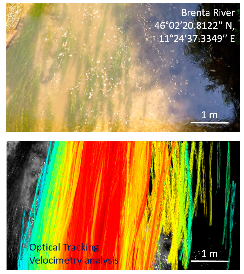
2.1.1. Controlled Outdoor Tests in the Brenta River

Experiments were performed on the Brenta River at the bridge “Ponte Zaccon”, Trento, Italy, ( 46 02 20.8122 North Latitude, 11 24 37.3349 East Longitude, 464.38 elevation in the WGS84 coordinate system) on 10 June 2015. Therein, a gauge station featuring an ultrasonic water level meter monitors the upper basin of the Brenta River ( 171.9 km 2 ), Figure 1a. At the bridge, the cross-section is 10.1 m wide and the river bed presents green filamentous algae, pebbles, and wood detritus. During the experiment, a constant water level of approximately 0.41 m was observed.
Experiments aimed at replicating ideal conditions for streamflow measurements with correlation- based optical approaches. Namely, woodchips were continuously deployed from the upstream side of the bridge throughout the entire cross-section. Particle diameter ranged within 10 to 15 pixels . Particles moved by less than 6 pixels between consecutive frames. On average, throughout an image sequence, particle density was approximately equal to 1.5 × 10 4 particles / total pixels (assuming an average particle diameter of 12 pixels ). Except for areas without tracers, a number of five to eight particles were on average present in interrogation windows of 32 × 32 pixels . The portable telescopic apparatus developed in [50] was installed on the downstream side of the bridge. The apparatus featured a GoPro Hero 4 Black edition camera oriented with its axis orthogonal to the water surface. A metre stick was placed on the right-side stream bank at the same level of the water surface for image photometric calibration. The camera was set to full HD ( 1920 × 1080 pixels ) resolution and at 50 Hz acquisition frequency. A video was recorded for over 4 minutes, and 12 video sequences of 20 s each and subsampled to 25 Hz were extracted out of the original footage. Analyzed images were 1430 × 1080 pixels in resolution (corresponding to a field of view of 7.1 × 5.3 m 2 ) and a bottom right area of 552 × 375 pixels displaying vegetation was masked with a black patch. Original RGB images were converted to grayscale intensity by eliminating hue and saturation information and retaining the luminance. To emphasize lighter particles against a dark background, images were gamma corrected to darken midtones [51], Figure 1b.

2.1.2. A Moderate Flood Event in The Tiber River

A video recorded at the gauge-cam station on the Tiber River underneath the bridge “Ponte del Foro Italico” in the city of Rome, Italy [52,53], on February 2015, at 7:40 a.m., was analyzed through OTV, Figure 1c. The gauge-cam station acquires one-minute long videos every ten minutes through a Mobotix FlexMount S15 weatherproof internet protocol camera. The camera comprises two optical modules with independent sensors and lenses, whereby only footage from the right-side L25 lens ( 82 angle of view and 4 mm focal length), which captured an area of 16.15 × 12.11 m 2 , was retained for the analyses. The optical axis is perpendicular to the water surface thus eliminating the requirement of orthorectification. Also, the gauge-cam station features a system of two <20 mW green ( 532 nm wavelength) lasers installed at 50 cm on both sides of the camera, Figure 1d. The lasers are activated for 20 s at the beginning of each video, and generate highly visible reference points located 1 m apart on the water surface. This laser system enables image photometric calibration. The frame acquisition frequency of the gauge-cam station is automatically adjusted based on external illumination conditions and, thus, varies for each captured clip. The overall frequency of the sequence of 410 images was estimated to be 6.95 Hz as a weighted average of each clip’s frequency. Such a relatively low frequency was sufficient to apply image-based streamflow measurement [18].
During the video, the transit of debris and vegetation was observable on the river surface due to a moderate flood. Generally, floating material tended to clump together to form objects on the order of 100 × 100 pixels . On average, material had a frame-by-frame displacement of less than 15 pixels . Over the entire image sequence, particle density was estimated to be 2.2 × 10 6 particles / total pixels (assuming an average particle diameter of 100 pixels ). Large scale floating material tended to transit on the right hand side of images. Image resolution was set to 1024 × 768 pixels for both optical modules. Images were affected by barrel distortion due to the wide-angle L25 lens. Fisheye distortion was removed using the Adobe Photoshop “Lens correction” filter. Also, frames were further trimmed to 865 × 530 pixels to remove highly distorted borders, Figure 1e.

2.2. Optical Tracking Velocimetry

2.2.1. Feature Detectors

Feature identification revolves around three main phases. First, points of interest are detected based on distinctive locations inside images. For instance, corners and junctions are frequently considered candidate features [54]. Then, the neighborhood of the feature is described as a vector and finally matched among different images, whereby the matching consists of computing a distance between vectors. All of these phases are affected by noise and, depending on the selection of the neighborhood, may require diverse computational times. Outdoors, image noise is considerable and feature identification plays a key role in the computation of trajectories and flow velocity. Also, even if several comparisons among feature detectors are available in the literature [55], changing illumination and the presence of fluid flow in streamflow images pose serious challenges that have been rarely investigated. Thus, in order to provide reliable guidelines for image-based streamflow observations, we assessed the performance of five different feature detectors that are highly popular in computer vision.
The good features to track (GFTT) approach identifies features based on their change of appearance between subsequent images. In this method, good features are the ones that can be more reliably tracked in image sequences, thus circumventing the requirement to define corners and points of interest in images [56]. Further, GFTT assumes an affine motion model, where features can be identified not only if they translate but also if images display deformation. The scale invariant feature transform (SIFT) is an efficient object recognition system that transforms images into large collections of local feature vectors. Features are invariant to translation, scaling, rotation, and moderately invariant to illumination changes and affine projections [57]. Even if not as computationally efficient as alternative algorithms, this approach has proved successful in numerous computer vision applications [58]. The features from accelerated segment test (FAST) directly addresses computation efficiency by a machine learning approach that yields high quality features [59]. The algorithm classifies image corners by considering a circle of sixteen pixels around a corner candidate and evaluating the intensity of each pixel. The speeded-up robust features (SURF) stems from previous feature detectors and improves their scale and in-plane rotation invariance [60]. Similarly, the oriented FAST and rotated binary robust independent elementary features (ORB) detector builds on FAST and exhibits orientation invariance and higher robustness to noise [61].
The robustness of the feature detection approach in case of high variance between successive frames was investigated by subsampling the image sequences of a representative video on the Brenta River at 12.5 Hz and 8.3 Hz . Reducing the frame frequency is crucial to minimize computational times, thus enabling real-time and continuous image processing that is of paramount importance to capture the evolving dynamics of hydrological processes. However, lower acquisition frequencies also yield an increased difference between successive frames, thus invalidating the assumption of intensity constancy. While the Lucas-Kanade approach can generally be adjusted to frequency to partially mitigate this issue, we identified the minimum frequency at which OTV led to meaningful results. Similar to frame acquisition frequency, image resolution greatly impacts computational times and the suitability of the image processing method for real-time operation. To this end, we subsampled the resolution of the image sequences to 720 × 953 pixels and 576 × 763 pixels . We then ran OTV with the five different feature detectors on the subsampled frame sequences.
To fully inspect the performance of the detectors, we also evaluated their effectiveness at frame-by-frame feature identification on a consistent representative image sequence on the Brenta River. In our test, we computed the average number of features identified by each detectors over the entire frame sequence. In addition, to verify if identified features also pertained to actual objects, we compared the number of detected features to the total number of trajectories. Specifically, we set the maximum number of trackable features among subsequent frames to 20,000. We then summed the total number of trajectories output by the method for different feature detectors. Results were also benchmarked to features randomly selected in the field of view, where the maximum number of randomly identifiable features in each frame was again set to 20,000. Similar tests have already been adopted in the literature to compare the performance of different detectors and inform their selection [62]. Our test was executed on full HD images recorded at 25 Hz .

2.2.2. Tracking Approach

The Lucas-Kanade algorithm is a sparse first-order differential technique that computes spatio-temporal derivatives of image intensity. The method assumes that image intensity, I ( x , t ) , a function of both position, x = ( x , y ) , and time, t, is conserved. Intensity constancy in image translation can be formulated as I ( x , t ) = I ( x v t , 0 ) , whereby v = ( u , v ) T indicates velocity in ( x , y ) [20]. More generally, the optical flow equation, d I ( x , t ) / d t = 0 , is expressed as a gradient constraint equation,
I ( x , t ) · v + I ( x , t ) t = 0
where I ( x , t ) and I ( x , t ) t indicate partial space and time derivatives and I · v denotes the dot product. According to [63], the residual function between images can be solved by the weighted least squares principle, where weights are assigned to image subsets. The weighting procedure gives more importance to pixels in the center of the subset.
In case of natural streamflow videos, images may display large pixel motion, which may lead to inaccurate optical flow computation. To this end, we used the pyramidal Lucas-Kanade approach where image resolution can be subsampled up to four levels [64]. Optical flow is then computed at the lower image resolution and then propagated up to the original image. Basically, the initial guess for pixel displacement is refined in a recursive fashion at higher resolution.
The algorithm was implemented in the open source computer vision (OpenCV) library in C++. We used the pyramidal approach up to the fourth level with a search window of 15 × 15 pixels in size. Features identified through the five detectors were used as input to the method and then matched in successive images. The iterative Lucas-Kanade algorithm was run until a maximum number of 20 iterations or when the search window moved by less than 0.03 pixels . Features were filtered out if the relative gradient matrix had a minimum eigenvalue less than 0.001 [64].

2.2.3. Trajectory-Based Filtering

Once feature trajectories were determined as in Section 2.2.1 and Section 2.2.2, they were post-processed through a filtering procedure developed in [18] for PTV results. Similar to [65], the procedure aims at retaining trajectories for velocity estimation only if they exhibit minimum variance of length and angle of travel between successive images, and if the detected features proceed for a minimum length in the field of view. The camera field of view is assumed to be directed with its width along the river cross-section. Also, detected features are supposed to move forward (that is, their trajectories should be fairly orthogonal to the river cross-section). These simple assumptions aim at reducing “false” trajectories that may bias velocity results. In fact, slanted trajectories with respect to the stream cross-section were frequently found to pertain to agglomerated features that separate while moving in the field of view [66].
The filtering constraints can be summarized as follows. When two successive frames (that is, frames k and k 1 ) are considered, feature position vectors X k and X k 1 should satisfy the following condition:
arctan ( X k X k 1 ) · j ( X k X k 1 ) · i > π 4
whereby j and i are unit vectors orthogonal and parallel to the river cross-section, respectively. Equation (2) is verified between each pair of frames during the analysis. Trajectories are further selected based on their length and slant. Namely, we only retain trajectories slanting up to 80 from the river cross-section and that extend for at least 20% of the height of the field of view ( H ). The first condition is imposed through
arctan ( X end X start ) · j ( X end X start ) · i > 4 9 π
whereby X end and X start indicate the feature position vectors in the final and first images of the trajectory, respectively. The length of the trajectory is validated through
X end X start > 1 5 H .
To minimize computational time, filtering through Equations (3) and (4) is implemented as soon as tracking of a selected feature through the Lucas-Kanade algorithm is ended. Threshold values in Equations (2)–(4) can be opportunely adjusted to account for the specific experimental conditions.
Streamflow velocity for each trajectory (V) is then determined as
V = X end X start Δ t
where Δ t is the time interval between the final and first images of the trajectory. Time-averaged cross-sectional profiles obtained with OTV and the five different feature detectors were tested for statistical significance through the analysis of variance (ANOVA), with level of significance, p, set to p < 0.05 .

2.3. Alternative Algorithms

Video data were processed with alternative correlation-based algorithms that are frequently implemented in hydrological studies. Specifically, image sequences were analyzed with LSPIV, PTV, and with the recently introduced PTV-Stream approach. PTV analyses were, in turn, applied both without (“Unfiltered PTV”) and with (“Filtered PTV”) the trajectory-based filtering procedure. Details on the procedures and implementation of LSPIV and PTV can be found in [18], while the PTV-Stream approach as well as its implementation on the Brenta and Tiber Rivers are presented in [19]. On the Brenta River, LSPIV was executed on sequences subsampled at 12.5 Hz and adopting the 1–2, 2–3 sequencing style. Standard direct cross-correlation was computed by setting the interrogation area to 32 × 32 pixels and the grid size to 16 × 16 pixels . The 2 × 3 -point Gaussian fit was used as sub-pixel displacement peak estimator. Upper and lower thresholds ( u ¯ ± 3 σ u , with u ¯ the mean velocity for each analyzed frame pair and σ u its standard deviation) were applied to velocity results. Consistent parameters were set to analyze the video of the Tiber River.
PTV entailed particle identification through cross-correlation with a symmetric Gaussian kernel (intensity grayscale level set to 130, standard deviation to 12 pixels , and correlation threshold set to 0.5 ). Further, particle tracking was implemented using cross-correlation by interrogation area (interrogation area set to 20 pixels , cross-correlation threshold to 0.4 , and neighbor similarity percentage to 20 % ). Analysis of the Tiber River image sequence with PTV encompassed consistent approach and parameters. The intensity grayscale level was set to 90 while all other parameters were consistent with the analysis on the Brenta River. PTV-Stream was implemented on videos of the Brenta and Tiber Rivers by setting the luminance threshold for particle identification to ± 50 and the particle area threshold to 35 pixels . Frame-by-frame changes in particle areas were set to less than 20 % or larger than 120 % and the search area was set to 20 × 100 pixels .

2.4. Velocity Data Extraction and Comparison

To offer a comparison among different image-based techniques for data collected on the Brenta River, the field of view was divided into eight parallel vertical regions 100 pixels-wide each. Such regions were selected in the center of the stream to exclude areas close to river banks, where tracers were scarce. Average velocities and standard deviations inside regions were computed for each technique. Specifically, velocities from OTV, PTV, and PTV-Stream were computed by averaging values obtained from Equation (5) for each trajectory laying in the vertical regions. Regarding LSPIV, time-averaged surface flow velocity maps were developed for each of the 12 image sequences. The average velocity and standard deviation were computed by intersecting time-averaged maps with vertical regions and averaging PIV cell values laying in such regions. Finally, for each method, we averaged values with respect to the 12 image sequences.
Image-based data were validated against velocities measured with an OTT Hydromet C2 current meter captured 3 cm below the water surface and at four locations along the stream cross-section up to 3.5 m from the right-side river bank. Twelve replicates of the current meter measurements were performed at each location; average velocities ( v ¯ b ) and standard deviations ( σ b ) are reported in Table 1.
Average velocity and standard deviation data on the Tiber River were obtained by averaging over the entire LSPIV time-averaged map and over the trajectories estimated with OTV, PTV, and PTV-Stream. Results were compared to measurements from an RVM20 speed surface radar installed next to the gauge-cam station that recorded an average surface velocity of 2.33 m / s during the experiment.

3. Results

In this Section, we report results for the Brenta and Tiber Rivers. For each case study, we first present velocimetry results obtained by analyzing video data with OTV. Then, we illustrate the performance of the different feature detectors and tracking approach. Finally, we compare velocity estimations to results from LSPIV, PTV, and PTV-Stream.

3.1. Assessment of OTV through Controlled Outdoor Tests in the Brenta River

OTV enabled successful extraction of the surface flow velocity of the Brenta River in moderate flow conditions. This is remarkable since experimental videos featured homogeneously and continuously seeded surfaces, which are inherently advantageous to correlation-based LSPIV and PTV rather than to optical flow [34]. Nonetheless, a considerable number of trajectories (on the order of 1000) were computed through OTV in each image sequence. All retained trajectories covered more than 20 % of the field of view and were several orders of magnitude more numerous than trajectories obtained with the filtered PTV approach illustrated in [18]. Therefore, OTV was not severely affected by the absence of continuous patterns in images nor by noise due to water reflections, and it may be suitable for streamflow measurements in challenging environmental conditions.

3.1.1. Average Surface Streamflow Velocity

Figure 2 illustrates trajectories computed by OTV with the five different feature detectors for a representative image sequence out of the 12 recorded on the Brenta River. The colorbar indicates the velocity of each trajectory calculated as in Equation (5). Left-hand plots display all trajectories identified by the method, while plots on the right-side only report trajectories that satisfy the filtering constraints. All techniques successfully reconstruct the surface flow velocity profile in the stream reach, with faster trajectories found in the center of the stream and slower ones close to the banks. Plots of unfiltered data report numerous low-velocity trajectories close to the left-side bank of the stream, where the stream bed is rich in permanent vegetation.
FAST-based OTV successfully identifies and tracks features located at the bottom of images in the shadowy area below the stream bridge, dashed rectangle in Figure 1b. This suggests that FAST is robust to noise in the illumination conditions of the water surface. SIFT-based OTV proves instead the most affected by changes in illumination conditions since many trajectories only start above the bridge shadow. SURF and GFTT-based OTV show several filtered trajectories close to the right-side stream bank, where the transit of artificially-deployed wood chips was rare. Thus, such detectors identify features that do not necessarily exhibit a higher contrast with respect to the background, which is a crucial property in case of unseeded water surfaces.
For a representative image sequence, in Figure 3, trajectories retained after the filtering procedure are reported for each vertical region and all feature detectors. Consistent with Figure 2, SURF and GFTT present a higher number of trajectories close to the right-side stream bank as compared to alternative algorithms. The SIFT technique yields the highest number of trajectories in three vertical bands out of eight, while the FAST algorithm leads to the lowest number of trajectories in seven vertical regions.
Average surface flow velocity estimations obtained by OTV with the five feature detectors for the 12 image sequences are reported in Figure 4. In Figure 4a, OTV results are illustrated for all the detectors along with current meter data (black dashed line). The root mean square error (RMSE) values between OTV results and the current meter data are also reported. In Figure 4b, the coefficient of determination ( R 2 ) values computed between results from each feature detector and the FAST method are showed. Average velocities are in good agreement among all procedures, with an average of 0.47 m / s . Such a value is slightly above the current meter measurements close to the center of the stream, which were taken at a depth of a few centimeters below the water surface. All the approaches also exhibit similar standard deviations (error bars in Figure 4a) and R 2 values. By analyzing the time-averaged cross-sectional profiles in Figure 4a through ANOVA, the difference among the techniques did not result statistically significant, thus supporting that all feature detectors captured the general behavior of the flow.

3.1.2. Subsampled Video Acquisition Frequency

On average, particles moved by less than 6 pixels between consecutive frames in the Brenta River. Minimum and maximum velocities estimated with all detectors were 0.157 m / s and 0.716 m / s , respectively. By subsampling the acquisition frequency to 12.5 Hz and 8.3 Hz , frame-by-frame displacement increased to 12 and 18 pixels for the maximum velocity and from to 2.5 and 3.8 pixels for the minimum velocity. In Figure 5, time-averaged cross-sectional profiles are reported for the five detectors and the three acquisition frequencies. Further, RMSE values between OTV results and current meter data and R 2 values computed with respect to the results at 25 Hz are showed. Specifically, a 1430 × 1080 pixels image sequence at frequencies of 25 Hz , 12.5 Hz , and 8.3 Hz was analyzed. The average velocity over the cross-section generally decreases up to a minimum of 0.44 m / s in case of the ORB detector and at the frequency of 8.3 Hz . On the other hand, the average standard deviation is not affected by frequency reduction, and therefore, even if the number of trajectories decreases, the filtering procedure is successful at retaining only reliable trajectories. Average velocities obtained with different feature detectors at the same frequency were not statistically different. Even if, at low frequencies, average velocities tended to decrease, differences between average velocities obtained with consistent feature detectors on frames subsampled at different frequencies were again not statistically significant ( p > > 0.05 ). Below the frequency of 7–8 Hz, OTV led to a sharp decrease in average velocities well below realistic values.

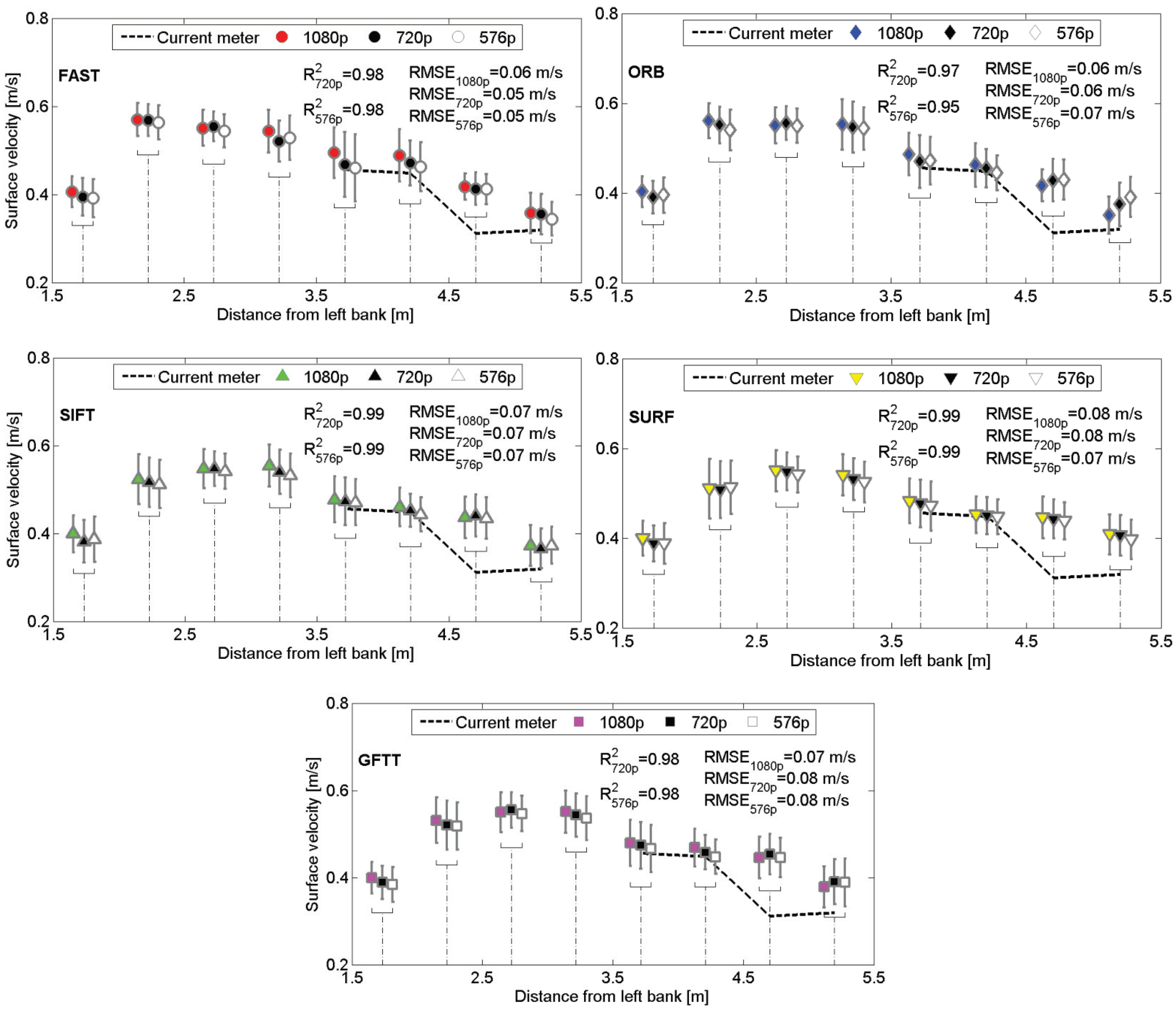
3.1.3. Subsampled Image Resolution

In Figure 6, time-averaged cross-sectional profiles are reported for the five detectors and three image resolutions: 1080 × 1430 pixels , 720 × 953 pixels , and 576 × 763 pixels . Specifically, a 25 Hz image sequence was sampled at 1430 × 1080 pixels , 720 × 953 pixels , and 576 × 763 pixels in resolution. RMSE values between OTV results and current meter data and R 2 values computed with respect to the results at 1080 × 1430 pixels resolution are also showed in Figure 6. In the analysis of lower-resolution images, input parameters to the Lucas-Kanade algorithm and the trajectory-based filtering procedure were consistent with the ones adopted for images at the original resolution.
The approach is minimally affected by decreased resolution and average velocities and standard deviations are consistent with values obtained from full HD images. No statistically significant differences are observable among average velocities obtained from consistent feature detectors on images at different resolutions.

3.1.4. Feature Detector Performance

Table 2 reports the average number of features identified in individual frames with the five different detectors in a representative image sequence on the Brenta River. Also, the total number of tracked features in the entire image sequence are presented (we set the maximum number of frame-by-frame detectable features to 20,000). The ORB detector is the most efficient at sensing features in images, with almost twice the number of features detected with FAST. On the other hand, SIFT and GFTT are the least efficient at identifying features but yield the highest number of tracked trajectories in the image sequence. Thus, such approaches accurately identify objects moving on the water surface whose trajectories were realistic and retained through the filtering procedure. Randomly selected features also lead to a high number of tracked features retained in the filtering phase. Generally, the ORB detector results as the most affected by noise since a large number of the detected features are filtered out from the computation (below the threshold of 20,000). The FAST technique instead leads to an approximately consistent number of identified and then tracked features. Also, this is the most computationally efficient technique that took less than a fifth of the time requested by the SIFT-based approach to process the image sequence. Randomly selecting features in the field of view also proves more computationally expensive than the FAST detector. On average, PTV techniques led to the identification of less than 70 features per frame. Such a value was further decreased upon trajectory-based filtering.

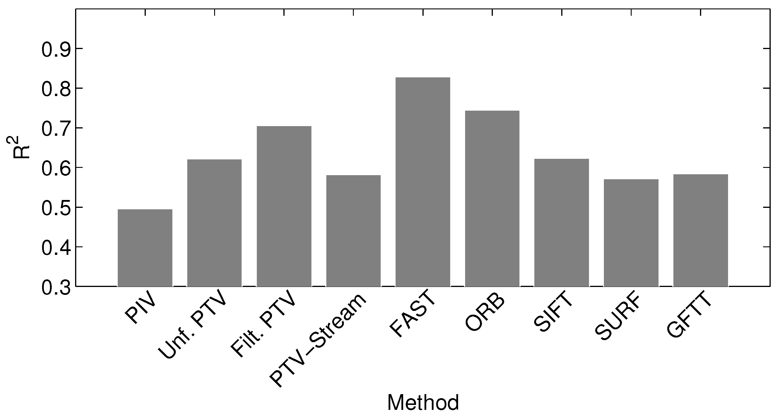
3.1.5. Comparison to Alternative Velocimetry Algorithms

In Figure 7, time-averaged cross-sectional profiles obtained with OTV are averaged with respect to the 12 image sequences and compared to alternative algorithms and the benchmark current meter measurements. RMSE and R 2 values computed between each method and the current meter data are also reported. The behavior of OTV techniques is generally consistent among different detectors. Generally, OTV velocity estimates are slightly higher than benchmark measurements since the current meter was deployed at 3 cm below the water surface. Consistent with PTV data, OTV largely overestimates water surface velocity at 2 m from the right-side bank, where stream bed irregularities may have influenced measurements with the current meter. Filtered PTV data exhibit the lowest standard deviation probably due to the fact that much less trajectories are retained in the computation with respect to OTV and unfiltered PTV. Unfiltered PTV instead shows the highest standard deviation, and therefore, cross-correlation with a gaussian mask implemented in PTVLab [16] may not be ideal to detect features on water surfaces in outdoor conditions. The recently introduced PTV-Stream technique is in general agreement with OTV and PTV data but leads to higher standard deviations. At 1 m from the right-side stream bank, only one trajectory is computed with PTV-Stream and, therefore, the standard deviation is null. Finally, results from LSPIV are generally lower than benchmark measurements as illustrated in [18].
In Figure 8, R 2 values computed between each approach and the benchmark data obtained with the current meter are illustrated. FAST-based OTV results exhibit the highest similarity to reference data ( R 2 = 0.83 ). Good performance is also achieved with ORB-based OTV ( R 2 = 0.74 ) and the filtered PTV ( R 2 = 0.70 ). The other PTV and OTV approaches present R 2 values approximately equal to 0.60. LSPIV results yield R 2 = 0.49 .

3.2. Proof of Concept Moderate Flood in the Tiber River

3.2.1. OTV Observations

Figure 9 displays unfiltered and filtered trajectories generated with OTV and the five different feature detectors for the video on the Tiber River. The filtering procedure successfully eliminates the influence of stationary reflections in the field of view by removing the low-velocity trajectories located on the left of the field of view. On the other hand, the high velocity area is consistently identified through all detectors on the right hand side of the image sequence. This region was also rich in floating sediments, and several objects (debris, floating vegetation, etc.) could be observed over the entire duration of the video. Since many trajectories do not extend for the entire field of view, it can be noted that OTV is influenced by the bridge shadow that created two regions at different illumination parallel to the image width, dashed rectangle in Figure 1e.

3.2.2. Comparison to Alternative Velocimetry Algorithms

Table 3 reports all the values of average velocity and standard deviations obtained with the different velocimetry approaches for the video of the moderate flood in the Tiber River. All methods severely underestimate the actual velocity and this is probably due to the variable frame acquisition frequency, that considerably influences velocity estimation. Remarkably, the performance of techniques that involve the trajectory-based filtering procedure is much better than LSPIV and unfiltered PTV (Unf. PTV in Table 3). Thus, it can be inferred that, in challenging conditions, imposing a few constraints on the general behavior of the flow may be highly beneficial for velocity estimations. The low standard deviation observed for PTV-Stream can be explained by the fact that only a meagre number of trajectories (slightly more than 20) are retained by the filtering procedure for velocity computation. In case of filtered PTV (Filt. PTV in Table 3), slightly less than 70 trajectories are retained for the computation against an average of more than 175,000 in case of OTV.

4. Discussion and Recommendations

4.1. Suitability of OTV for Streamflow Observations

OTV has proved efficient at providing information on the surface flow kinematics in outdoor conditions based on video footage captured in two different experimental settings. In case of highly seeded surfaces, where optical flow schemes do not typically outperform correlation-based methods, the combination of automated feature detectors, sparse Lucas-Kanade, and trajectory-based filtering yielded accurate velocity estimations, generally in agreement with benchmark manual data. In case of the moderate flood on the Tiber River, the scheme was severely affected by unstable acquisition frequency and velocities were largely underestimated. In experiments on the Brenta River, optical flow-based velocities displayed very low standard deviations, thus supporting the evidence that the variable frequency of the footage of the Tiber River may have biased the computation of surface velocity. In both sets of experiments, the method generated up to several thousands of trajectories even in regions of the field of view where the transit of actual objects could not be visually observed. This fact is of fundamental importance in case of difficult-to-access environments, where deploying tracers may be hampered. As expected, the need for a trajectory-based filtering procedure in outdoor conditions was essential to guarantee that objects rather than stationary water reflections or noise due to illumination were detected and tracked.
In both data sets, the different feature detectors led to consistent results. The FAST approach proved as the most efficient due to its balance between identified and effectively tracked and filtered features. Computational times required by the FAST implementation were generally shorter than other techniques, even with respect to the random selection of features in the field of view. The SIFT and ORB algorithms were more significantly affected by changes in illumination, which are typical in natural settings. The SIFT approach was successful at identifying numerous features but then also led to increased processing times. Interestingly, the SURF and GFTT detectors recovered many features in regions that did not present very high contrast. This fact could be advantageous in case of mirror-like uniform water surfaces and low flow regimes, where the transit of floaters is much scarcer.
The methodology proved relatively insensitive to image resolution while acquisition frequency was found to be a key control to its performance. In experiments on the Brenta River, a frame acquisition frequency lower than 7–8 Hz led to a sharp decrease in velocity estimation. Similar findings have also been observed in PTV-Stream implementations [19]. Of course, the selection of the frame acquisition frequency is related to the size of the field of view and to flow velocity. Therefore, based on our findings, a preliminary analysis on subsampled video sequences may be beneficial to inform the installation of permanent gauge-cams or instrumentation in the field.

4.2. Comparison to Alternative Velocimetry Algorithms

OTV results were generally in good agreement with the filtered PTV method and PTV-Stream. The improved performance of procedures that involve filtering of the trajectories confirms that this is a crucial phase to retain reliable trajectories and, therefore, generate accurate velocity estimations. In addition, the filtering procedure only requires minimal information that can be easily gathered by a preliminary inspection of the field of view. Different from filtered PTV and PTV-Stream, OTV allowed for generating a much more significant number of trajectories, which is beneficial to estimate the uncertainty of velocity estimations, and it also required less input since the detection and tracking is fully automated. Another advantage with respect to traditional PTV is the independence of OTV on the shape and size of the tracers that allows for improved performance in case of naturally occurring floaters [34,39]. Compared to LSPIV and traditional unfiltered PTV, OTV led to more robust velocity estimations with lower standard deviations. Our findings demonstrate that traditional correlation-based methods suffer from noise, dishomogeneously seeded surfaces, and from the irregularities that are typical of outdoor settings. While such methods may be efficiently implemented in controlled settings, OTV may instead be a valid alternative in complex settings.
OTV was also the most computational efficient among the methods presented in this work. Processing an image sequence of the Brenta River required approximately 2 min on a personal computer (×86_64 architecture with an AMD Ryzen 7 1700X eight-core processor, CPU ranging from 2.2 GHz to 3.4 GHz , 2 threads per core, and total memory of 16.4 Gb ) against the 17 min (with a deviation of 7 min on an ASUS laptop with an Intel Core i7 2670QM Processor, CPU ranging from 2.2 GHz to 3.1 GHz , 2 threads per core) taken by PTV-Stream, which is a custom-made procedure developed in Java. The computational times required for PTV and LSPIV processing with PTVLab and PIVLab are two orders of magnitude longer than OTV.

4.3. Criticalities and Future Developments

The efficiency and robustness of OTV support its implementation for real-time streamflow observations through gauge-cams. We foresee that processing units may be integrated in prototypes similar to the one installed on the Tiber River to generate spatially distributed velocity data at high temporal resolution. Of course, extensive calibration and optimization of the algorithms would be necessary to enable fast computation on simple processing units. In addition, further efforts are necessary to validate the performance of the feature detectors and the tracking scheme in even more diverse flow regimes and illumination settings. For instance, generating results in case of extremely scarce illumination or at night is still an open problem. In some other instances, the presence of image subregions that display highly different illumination, such as, for instance, underneath bridges, may lead to shorter trajectories (that is, the tracking is typically interrupted when the feature crosses two areas where the average intensity is remarkably different). Similarly, rapid changes in the illumination may introduce several problems in recovering long and reliable trajectories. On the other hand, preliminary tests on mirror-like surfaces have highlighted that the absence of objects visible with a naked eye is not crucial to apply OTV. In fact, the feature detectors successfully identify minimal changes in the intensity of the water surface that can be regarded as tracers.
OTV results were developed both in case of shallow depth (the Brenta River water level was 0.41 m deep at the time of the experiments) and rather deep stream (the water level was greater than 7 m in the Tiber River at the time of the experiment). In the Brenta River, bottom-reflected radiance was non-negligible; however, it did not affect the accuracy of surface flow velocity measurements. On the other hand, in the Tiber River, higher turbidity and depth should enhance the visibility of surface tracers and flow velocity estimation. Nonetheless, in this latter case, the irregular frequency of image sequences controlled the accuracy of the method. Interestingly, when the bottom-reflected radiance is dominant (that is, especially in shallow streams) image data could also be utilized for stream depth retrieval [67], thus leading to a flexible and integrated discharge measurement approach.
Establishing standard protocols and guidelines for the implementation of OTV in different settings is another important issue to be addressed in the future. Even if innovative observational techniques and approaches are blossoming in hydrology [68], many of these multidisciplinary methods are not validated and taken to the maturity of traditional techniques. In this respect, very few initiatives are currently aiming at leveraging the potential of new methods through the coordinated harmonization of protocols and techniques [69].
Another criticality and future endeavor entails the computation of flow discharge and the establishment of rating curves from OTV. Even if some proof-of-concept experiments have been conducted to demonstrate discharge estimation from image-based methods [70,71], this is still an open problem in hydrology. We foresee that the integration of OTV and the methodologies by [72,73] for the estimation of mean velocity in open channels may be beneficial for advancing current practice in remote hydrological observations.

5. Conclusions

A novel optical flow scheme, optical tracking velocimetry (OTV), was introduced for remote streamflow observations in natural settings. The approach encompasses automated feature detection, tracking through the differential sparse Lucas-Kanade algorithm, and trajectory-based filtering from a priori known information on the flow direction. The methodology was tested on two diverse image data sets: a set of videos collected on the Brenta River, where artificial seeding was provided, and the footage of a moderate flood captured by a gauge-cam on the Tiber River. Average surface flow velocity estimations on the Brenta River were in good agreement with the current meter measurements for all the five feature detectors. Velocity results for the Tiber River were instead more severely influenced by unstable frame acquisition frequency.
Different from alternative correlation-based approaches, OTV led to a number of trajectories on the order of several thousands. Out of the tested feature detectors, the FAST algorithm proved the most computationally efficient and stable in terms of number of features identified and then tracked. OTV was only mildly affected by low image resolution and led to acceptable results even in case of rather low image frequencies (7–8 Hz with respect to an average surface flow velocity on the order of 0.4–0.5 m/s). The methodology highly benefited from a posteriori trajectory-based filtering that only retains trajectories pertaining to actual objects transiting in the field of view. OTV is inherently suited for real-time implementations on gauge-cams, even if further validation and standardization of protocols are necessary in a wide array of hydrological settings.

Supplementary Materials

The following is available online at https://zenodo.org/record/2387110#.XBje5M2VOUk, Video S1: Brenta_analysis.avi.

Author Contributions

Conceptualization, F.T. (Flavia Tauro), S.M., E.T. and S.G.; Methodology, F.T. (Fabio Tosi), F.T. (Fabio Tosi), S.M., R.P. and S.G.; Software, F.T. (Flavia Tauro), F.T. (Fabio Tosi), and R.P.; Validation, F.T. (Flavia Tauro) and S.G.; Formal Analysis, F.T. (Flavia Tauro), F.T. (Fabio Tosi), R.P.; Resources, E.T., S.M. and S.G.; Data Curation, F.T. (Flavia Tauro), F.T. (Fabio Tosi) and R.P.; Writing—Original Draft Preparation, F.T. (Flavia Tauro); Writing—Review & Editing, F.T. (Flavia Tauro), F.T. (Fabio Tosi), S.M., E.T., R.P. and S.G.

Funding

This work was supported by POR-FESR 2014–2020 n. 737616 INFRASAFE and by the “Departments of Excellence-2018” Program (Dipartimenti di Eccellenza) of the Italian Ministry of Education, University and Research, DIBAF—Department of University of Tuscia, Project “Landscape 4.0—food, wellbeing and environment”.

Acknowledgments

The authors gratefully thank Andrea Petroselli for help with the experiments, and Centro Funzionale—Regione Lazio for radar data availability.

Conflicts of Interest

The authors declare no conflict of interest. The founding sponsors had no role in the design of the study; in the collection, analyses, or interpretation of data; in the writing of the manuscript, and in the decision to publish the results.

References

  1. Clarke, T.R. Uncertainty in the estimation of mean annual flood due to rating-curve indefinition. J. Hydrol. 1999, 222, 185–190. [Google Scholar] [CrossRef]
  2. Di Baldassarre, G.; Montanari, A. Uncertainty in river discharge observations: A quantitative analysis. Hydrol. Earth Syst. Sci. 2009, 13, 913–921. [Google Scholar] [CrossRef]
  3. McMillan, H.; Freer, J.; Pappenberger, F.; Krueger, T.; Clark, M. Impacts of uncertain river flow data on rainfall-runoff model calibration and discharge predictions. Hydrol. Process. 2010, 24, 1270–1284. [Google Scholar] [CrossRef]
  4. Hairsine, P.B.; Rose, C.W. Modeling water erosion due to overland flow using physical principles: 1. Sheet flow. Water Resour. Res. 1992, 28, 237–243. [Google Scholar] [CrossRef]
  5. Yorke, T.H.; Oberg, K.A. Measuring river velocity and discharge with acoustic Doppler profilers. Flow Meas. Instrum. 2002, 13, 191–195. [Google Scholar] [CrossRef]
  6. Czuba, J.A.; Foufoula-Georgiou, E.; Gran, K.B.; Belmont, P.; Wilcock, P.R. Interplay between spatial explicit sediment sourcing, hierarchical river-network structure, and in-channel bed material sediment transport and storage dynamics. J. Geophys. Res. Earth Surf. 2017, 122, 1090–1120. [Google Scholar] [CrossRef]
  7. Costa, J.; Spicer, K.; Cheng, R.; Haeni, F.; Melcher, N.; Thurman, E.; Plant, W.; Keller, W. Measuring stream discharge by non-contact methods—A proof-of-concept experiment. Geophys. Res. Lett. 2000, 27, 553–556. [Google Scholar] [CrossRef]
  8. Tauro, F.; Petroselli, A.; Grimaldi, S. Optical sensing for stream flow observations: A review. J. Agric. Eng. 2018, 49. [Google Scholar] [CrossRef]
  9. Legleiter, C.J.; Mobley, C.D.; Overstreet, B.T. A framework for modeling connections between hydraulics, water surface roughness, and surface reflectance in open channel flows. J. Geophys. Res. Earth Surf. 2017, 122, 1715–1741. [Google Scholar] [CrossRef]
  10. Legleiter, C.J.; Kinzel, P.J.; Nelson, J.M. Remote measurement of river discharge using thermal particle image velocimetry (PIV) and various sources of bathymetric information. J. Hydrol. 2017, 554, 490–506. [Google Scholar] [CrossRef]
  11. Adrian, R.J. Particle-imaging techniques for experimental fluid-mechanics. Annu. Rev. Fluid Mech. 1991, 23, 261–304. [Google Scholar] [CrossRef]
  12. Adrian, R.J. Twenty years of particle image velocimetry. Exp. Fluids 2005, 39, 159–169. [Google Scholar] [CrossRef] [Green Version]
  13. Raffel, M.; Willert, C.E.; Wereley, S.T.; Kompenhans, J. Particle Image Velocimetry. A Practical Guide; Springer: New York, NY, USA, 2007. [Google Scholar]
  14. Fujita, I.; Muste, M.; Kruger, A. Large-scale particle image velocimetry for flow analysis in hydraulic engineering applications. J. Hydraul. Res. 1997, 36, 397–414. [Google Scholar] [CrossRef]
  15. Lloyd, P.M.; Stansby, P.K.; Ball, D.J. Unsteady surface-velocity field measurement using particle tracking velocimetry. J. Hydraul. Res. 1995, 33, 519–534. [Google Scholar] [CrossRef]
  16. Brevis, W.; Niño, Y.; Jirka, G.H. Integrating cross-correlation and relaxation algorithms for particle tracking velocimetry. Exp. Fluids 2011, 50, 135–147. [Google Scholar] [CrossRef]
  17. DalSasso, S.F.; Pizarro, A.; Samela, C.; Mita, L.; Manfreda, S. Exploring the optical experimental setup for surface flow velocity measurements using PTV. Environ. Monit. Assess. 2018, 190, 460. [Google Scholar] [CrossRef] [PubMed]
  18. Tauro, F.; Piscopia, R.; Grimaldi, S. Streamflow observations from cameras: Large-scale particle image velocimetry or particle tracking velocimetry? Water Resour. Res. 2017, 53, 10374–10394. [Google Scholar] [CrossRef]
  19. Tauro, F.; Piscopia, R.; Grimaldi, S. PTV-Stream: A simplified particle tracking velocimetry framework for stream surface flow monitoring. Catena 2019, 172, 378–386. [Google Scholar] [CrossRef]
  20. Horn, B.K.P.; Schunck, B.G. Determining optical flow. Artif. Intell. 1981, 17, 185–203. [Google Scholar] [CrossRef] [Green Version]
  21. Barron, J.L.; Fleet, D.J.; Beauchemin, S.S. Performance of optical flow techniques. Int. J. Comput. Vis. 1994, 12, 43–77. [Google Scholar] [CrossRef] [Green Version]
  22. Chao, H.; Gu, Y.; Napolitano, M. A survey of optical flow techniques for robotics navigation applications. J. Intell. Robot. Syst. 2014, 73, 361–372. [Google Scholar] [CrossRef]
  23. James, M.R.; Pinkerton, H.; Robson, S. Image-based measurement of flux variation in distal regions of active lava flows. Geochem. Geophys. Geosyst. 2007, 8, Q03006. [Google Scholar] [CrossRef]
  24. Raaf, O.; Adane, A. The determination of rainy clouds motion using optical flow. In Nonlinear and Complex Dynamics; Springer: New York, NY, USA, 2011; pp. 179–191. [Google Scholar]
  25. Li, L.; Chen, S.; Mai, X.F. Sub-pixel precipitation nowcasting over Guangdong province using opitcal flow algorithm. In Proceedings of the IEEE International Geoscience and Remote Sensing Symposium (IGARSS), Fort Worth, TX, USA, 23–28 July 2017; pp. 4638–4641. [Google Scholar]
  26. Reinoso, J.F.; León, C.; Mataix, J. Optical flow algorithm as estimator of horizontal discrepancy between features derived from DEMs: Rivers and creeks as case study. Surv. Rev. 2013, 46, 149–154. [Google Scholar] [CrossRef]
  27. Mémin, E.; Pérez, P. Fluid motion recovery by coupling dense and parametric vector fields. In Proceedings of the 7th IEEE International Conference on Computer Vision, Kerkyra, Greece, 20–27 September 1999. [Google Scholar]
  28. Wildes, R.P.; Amabile, M.J.; Lanzillotto, A.M.; Leu, T.S. Recovering estimates of fluid flow from image sequence data. Comput. Vis. Image Understand. 2000, 80, 246–266. [Google Scholar] [CrossRef]
  29. Corpetti, T.; Heitz, D.; Arroyo, G.; Mémin, E. Fluid experimental flow estimation based on an optical-flow scheme. Exp. Fluids 2006, 40, 80–97. [Google Scholar] [CrossRef]
  30. Yuan, J.; Schnörr, C.; Mémin, E. Discrete orthogonal decomposition and variational fluid flow estimation. J. Math. Imaging Vis. 2007, 28, 67–80. [Google Scholar] [CrossRef]
  31. Liu, T.; Shen, L. Fluid flow and optical flow. J. Fluid Mech. 2008, 614, 253–291. [Google Scholar] [CrossRef]
  32. Sakaino, H. Fluid motion estimation method based on physical properties of waves. In Proceedings of the IEEE Conference on Computer Vision and Pattern Recognition, Anchorage, AK, USA, 23–28 June 2008. [Google Scholar]
  33. Doshi, A.; Bors, A.G. Robust processing of optical flow of fluids. IEEE Trans. Image Process. 2010, 19, 2332–2344. [Google Scholar] [CrossRef]
  34. Liu, T.; Merat, A.; Makhmalbaf, M.H.M.; Fajardo, C.; Merati, P. Comparison between optical flow and cross-correlation methods for extraction of velocity fields from particle images. Exp. Fluids 2015, 56, 166. [Google Scholar] [CrossRef]
  35. Bruhn, A.; Weickert, J.; Schnörr, C. Pattern Recognition. In Lecture Notes in Computer Science; Chapter Combining the Advantages of Local and Global Optic Flow Methods; Springer: Berlin, Germany, 2002; Volume 2449, pp. 454–462. [Google Scholar]
  36. Plyer, A.; Le Besnerais, G.; Champagnat, F. Massively parallel Lucas Kanade optical flow for real-time video processing applications. J. Real-Time Image Process. 2016, 11, 713–730. [Google Scholar] [CrossRef]
  37. Quénot, G.M.; Pakleza, J.; Kowalewski, T.A. Particle image velocimetry with optical flow. Exp. Fluids 1998, 25, 177–189. [Google Scholar] [CrossRef]
  38. Shindler, L.; Moroni, M.; Cenedese, A. Using optical flow equation for particle detection and velocity prediction in particle tracking. Appl. Math. Comput. 2012, 218, 8684–8694. [Google Scholar] [CrossRef]
  39. Bacharidis, K.; Moirogiorgou, K.; Sibetheros, I.A.; Savakis, A.E.; Zervakis, M. River flow estimation using video data. In Proceedings of the IEEE International Conference on Imaging Systems and Techniques (IST) Proceedings, Santorini, Greece, 14–17 October 2014. [Google Scholar]
  40. Chang, J.; Edwards, D.; Yu, Y. Statistical estimation of fluid flow fields. In Proceedings of the ECCV Workshop on Statistical Methods in Video Processing, Lyon, France, 21–26 July 2002; pp. 91–96. [Google Scholar]
  41. Bung, D.B.; Valero, D. Application of the optical flow method to velocity determination in hydraulic structure models. In Proceedings of the 6th International Symposium on Hydraulic Structures, Portland, OR, USA, 27–30 June 2016; pp. 240–249. [Google Scholar]
  42. Dérian, P.; Almar, R. Wavelet-based optical flow estimation of instant surface currents from shore-based and UAV videos. IEEE Trans. Geosci. Remote Sens. 2017, 55, 5790–5797. [Google Scholar] [CrossRef]
  43. Ghalenoei, E.; Hasanlou, M. Monitoring of sea surface currents by using sea surface temperature and satellite altimetry data in the Caspian Sea. Earth Obs. Geomat. Eng. 2017, 1, 36–46. [Google Scholar]
  44. Vogel, C.; Bauder, A.; Schindler, K. Optical flow for glacier motion estimation. In Proceedings of the ISPRS Annals of the Photogrammetry, Remote Sensing and Spatial Information Sciences (XXII ISPRS Congress), Melbourne, Australia, 25 August–1 September 2012; Volume I-3, pp. 359–364. [Google Scholar]
  45. Karvonen, J. Virtual radar ice buoys—A method for measuring fine-scale sea ice drift. Cryosphere 2016, 10, 29–42. [Google Scholar] [CrossRef]
  46. Krout, D.W.; Okopal, G.; Jessup, A.; Hanusa, E. Tracking drifting surface objects with aerial infrared and electro-optical sensors. In Proceedings of the 2012 Oceans, Hampton Roads, VA, USA, 14–19 October 2012; pp. 1–4. [Google Scholar] [CrossRef]
  47. Waghmare, A.; Naik, A.A. Water velocity measurement using contact and non-contact type sensor. In Proceedings of the 2015 Communication, Control and Intelligent Systems (CCIS), Mathura, India, 7–8 November 2015; pp. 334–338. [Google Scholar]
  48. Zhang, G.; Chanson, H. Application of local opticl flow methods to high-velocity free-surface flows: Validation and application to stepped chutes. Exp. Therm. Fluid Sci. 2018, 90, 186–199. [Google Scholar] [CrossRef]
  49. Perks, M.T.; Russell, A.J.; Large, A.R.G. Technical Note: Advances in flash flood monitoring using unmanned aerial vehicles (UAVs). Hydrol. Earth Syst. Sci. 2016, 20, 4005–4015. [Google Scholar] [CrossRef]
  50. Tauro, F.; Porfiri, M.; Grimaldi, S. Orienting the camera and firing lasers to enhance large scale particle image velocimetry for streamflow monitoring. Water Resour. Res. 2014, 50, 7470–7483. [Google Scholar] [CrossRef] [Green Version]
  51. Forsyth, D.A.; Ponce, J. Computer Vision: A Modern Approach; Pearson: Prentice Hall, NJ, USA, 2011. [Google Scholar]
  52. Tauro, F.; Petroselli, A.; Porfiri, M.; Giandomenico, L.; Bernardi, G.; Mele, F.; Spina, D.; Grimaldi, S. A novel permanent gauge-cam station for surface-flow observations on the Tiber River. Geosci. Instrum. Methods Data Syst. 2016, 5, 241–251. [Google Scholar] [CrossRef] [Green Version]
  53. Tauro, F.; Salvatori, S. Surface flows from images: Ten days of observations from the Tiber River gauge-cam station. Hydrol. Res. 2016, 48, 646–655. [Google Scholar] [CrossRef]
  54. Tuytelaars, T.; Mikolajczyk, K. Local invariant feature detectors: A survey. Found. Trends® Comput. Graph. Vis. 2008, 3, 177–280. [Google Scholar] [CrossRef]
  55. Mikolajczyk, K.; Schmid, C. A performance evaluation of local descriptors. IEEE Trans. Pattern Anal. Mach. Intell. 2005, 27, 1615–1630. [Google Scholar] [CrossRef] [PubMed] [Green Version]
  56. Shi, J.; Tomasi, C. Good features to track. In Proceedings of the IEEE Conference on Computer Vision and Pattern Recognition, Seattle, WA, USA, 21–23 June 1994. [Google Scholar]
  57. Lowe, D.G. Object recognition from local scale-invariant features. In Proceedings of the International Conference on Computer Vision (ICCV’99), Kerkyra, Greece, 20–27 September 1999; IEEE Computer Society: Washington, DC, USA, 1999; Volume 2, p. 1150. [Google Scholar]
  58. Valgren, C.; Lilienthal, A.J. SIFT, SURF & seasons: Appearance-based long-term localization in outdoor environments. Robot. Auton. Syst. 2010, 58, 149–156. [Google Scholar]
  59. Rosten, E.; Drummond, T. Machine learning for high-speed corner detection. In Proceedings of the ECCV, Graz, Austria, 7–13 May 2006. [Google Scholar]
  60. Bay, H.; Ess, A.; Tuytelaars, T.; Van Gool, L. Speeded-up robust features (SURF). Comput. Vis. Image Understand. 2008, 110, 346–359. [Google Scholar] [CrossRef]
  61. Rublee, E.; Rabaud, V.; Konolige, K.; Bradski, G. ORB: An efficient alternative to SIFT or SURF. In Proceedings of the 2011 International Conference on Computer Vision, Barcelona, Spain, 6–13 November 2011; pp. 2564–2571. [Google Scholar]
  62. Nourani-Vatani, N.; Borges, P.V.K.; Roberts, J.M. A study of feature extraction algorithms for optical flow tracking. In Proceedings of the Australasian Conference on Robotics and Automation, Wellington, New Zealand, 3–5 December 2012. [Google Scholar]
  63. Lucas, B.D.; Kanade, T. An iterative image registration technique with an application to stereo vision. In Proceedings of the 7th International Joint Conference On Artificial Intelligence (IJCAI’81), Vancouver, BC, Canada, 24–28 August 1981; Morgan Kaufmann Publishers Inc.: Vancouver, BC, Canada, 1981; Volume 2, pp. 674–679. [Google Scholar]
  64. Bouguet, J.Y. Pyramidal Implementation of the Lucas Kanade Feature Tracker—Description of the Algorithm; Technical Report; Intel Microprocessor Research Labs: Santa Clara, CA, USA, 1999. [Google Scholar]
  65. Hassan, Y.A.; Canaan, R.E. Full-field bubbly flow velocity measurements using a multiframe particle tracking technique. Exp. Fluids 1991, 12, 49–60. [Google Scholar] [CrossRef]
  66. Tauro, F.; Grimaldi, S. Ice dices for monitoring stream surface velocity. J. Hydro-Environ. Res. 2017, 14, 143–149. [Google Scholar] [CrossRef]
  67. Niroumand-Jadidi, M.; Vitti, A.; Lyzenga, D.R. Multiple Optimal Depth Predictors Analysis (MODPA) for river bathymetry: Findings from spectroradiometry, simulations, and satellite imagery. Remote Sens. Environ. 2018, 218, 132–147. [Google Scholar] [CrossRef]
  68. Tauro, F.; Selker, J.; van de Giesen, N.; Abrate, T.; Uijlenhoet, R.; Porfiri, M.; Manfreda, S.; Caylor, K.; Moramarco, T.; Benveniste, J.; et al. Measurements and Observations in the XXI century (MOXXI): Innovation and multidisciplinarity to sense the hydrological cycle. Hydrol. Sci. J. 2018, 63, 169–196. [Google Scholar] [CrossRef]
  69. Manfreda, S.; McCabe, M.F.; Miller, P.E.; Lucas, R.; Madrigal, V.P.; Mallinis, G.; Ben Dor, E.; Helman, D.; Estes, L.; Ciraolo, G.; et al. On the use of unmanned aerial systems for environmental monitoring. Remote Sens. 2018, 10, 641. [Google Scholar] [CrossRef]
  70. Hauet, A.; Kruger, A.; Krajewski, W.; Bradley, A.; Muste, M.; Creutin, J.; Wilson, M. Experimental system for real-time discharge estimation using an image-based method. J. Hydrol. Eng. 2008, 13, 105–110. [Google Scholar] [CrossRef]
  71. Huang, W.C.; Young, C.C.; Liu, W.C. Application of an automated discharge imaging system and LSPIV during typhoon events in Taiwan. Water 2018, 10, 280. [Google Scholar] [CrossRef]
  72. Chiu, C.L. Application of entropy concept in open-channel flow study. J. Hydraul. Eng. 1991, 117, 615–628. [Google Scholar] [CrossRef]
  73. Moramarco, T.; Saltalippi, C.; Singh, V.P. Estimation of mean velocity in natural channels based on Chiu’s velocity distribution equation. J. Hydraul. Eng. 2004, 9, 42–50. [Google Scholar] [CrossRef]
Figure 1. (a) View and (b) representative processed image of the Brenta River; (c) location of the gauge-cam on the Tiber River; (d) camera and laser units of the gauge-cam, and (e) representative processed image. The white dashed rectangles in panels (b,e) indicate regions at darker intensity due to the bridge shadow.
Remotesensing 10 02010 g001
Figure 2. Unfiltered and filtered trajectories obtained with optical tracking velocimetry (OTV) and five different feature detectors for a representative video on the Brenta River. The colorbar indicates velocity magnitude for each trajectory computed as Equation (5). Flow direction is upwards.
Remotesensing 10 02010 g002
Figure 3. Number of trajectories per vertical region as obtained for a representative image sequence on the Brenta River with the five different feature detectors.
Remotesensing 10 02010 g003
Figure 4. (a) Time-averaged surface flow velocity cross-sectional profiles obtained by processing the 12 image sequences on the Brenta River with OTV. Error bars indicate standard deviations. The black dashed line illustrates average velocities obtained with the current meter. Root mean square error (RMSE) values between OTV results and the current meter data are reported. OTV data obtained from different feature detectors refer to consistent distances from the left stream bank as indicated with brackets and dash-dotted lines; (b) R 2 values computed between results from each feature detector and the features from accelerated segment test (FAST) method.
Remotesensing 10 02010 g004
Figure 5. Time-averaged surface flow velocity cross-sectional profiles obtained by processing the 12 image sequences on the Brenta River with OTV. Error bars indicate standard deviations. Black markers pertain to 12.5 Hz and white markers to 8.3 Hz . The black dashed line illustrates average velocities obtained with the current meter. RMSE values between OTV results and the current meter data are reported. R 2 values computed with respect to the results at 25 Hz are showed. OTV data obtained from sequences sampled at different frequencies refer to consistent distances from the left stream bank as indicated with brackets and dash-dotted lines.
Remotesensing 10 02010 g005
Figure 6. Time-averaged surface flow velocity cross-sectional profiles obtained by processing the 12 image sequences on the Brenta River with OTV. Error bars indicate standard deviations. Black markers pertain to 720 × 953 pixels resolutions and white markers to 576 × 763 pixels resolutions. The black dashed line illustrates average velocities obtained with the current meter. RMSE values between OTV results and the current meter data are reported. R 2 values computed with respect to the results at 1080 × 1430 pixels resolution are showed. OTV data obtained from sequences sampled at different resolutions refer to consistent distances from the left stream bank as indicated with brackets and dash-dotted lines.
Remotesensing 10 02010 g006
Figure 7. Time-averaged surface flow velocity cross-sectional profiles obtained by processing the 12 image sequences on the Brenta River with all approaches. RMSE and R 2 values computed between each method and the current meter data are reported.
Remotesensing 10 02010 g007
Figure 8. R 2 values computed between all the approaches and the benchmark current meter data.
Remotesensing 10 02010 g008
Figure 9. Unfiltered and filtered trajectories obtained with OTV and five different feature detectors for the video on the Tiber River. The colorbar indicates velocity magnitude for each trajectory computed as Equation (5). Flow direction is upwards.
Remotesensing 10 02010 g009
Table 1. Average benchmark velocities ( v ¯ b ) and standard deviations ( σ b ) measured with the current meter in the Brenta River. Measurement locations are at 1, 2, 2.7 , and 3.5 from the right-side river bank.
3.5 m 2.7 m 2 m 1 m
v ¯ b ( m / s ) 0.460.450.310.32
σ b ( m / s ) 0.040.030.020.02
Table 2. Frame-by-frame average number of detected features and total number of tracked features with optical tracking velocimetry (OTV) and six different feature detectors for a representative image sequence of 500 frames on the Brenta River.
MethodProcessing Time ( s )Frame-by-Frame Average Detected Features ( num )Total Tracked Features ( num )
FAST4319,09818,076
ORB6137,96818,325
SIFT235765624,119
SURF8310,07621,887
GFTT67778824,747
Random5020,00023,215
Table 3. Average velocity, standard deviation, number of trajectories, and processing time for the video on the Tiber River and the five different feature detectors, as well as all velocimetry approaches. The benchmark radar velocity was 2.33 m / s .
FASTORBSIFTSURFGFTTLSPIVUnf. PTVFilt. PTVPTV-Stream
average velocity ( m / s )1.541.571.501.491.520.390.661.41.6
standard deviation ( m / s )0.320.380.360.340.350.070.270.20.09
trajectories ( num )214,884223,706163,599144,735149,83419,0006824
time ( s )3440944342>3000>3000>3000>1000

