Sea Surface Temperature Retrieval from the First Korean Geostationary Satellite COMS Data: Validation and Error Assessment


Abstract

1. Introduction
2. Data
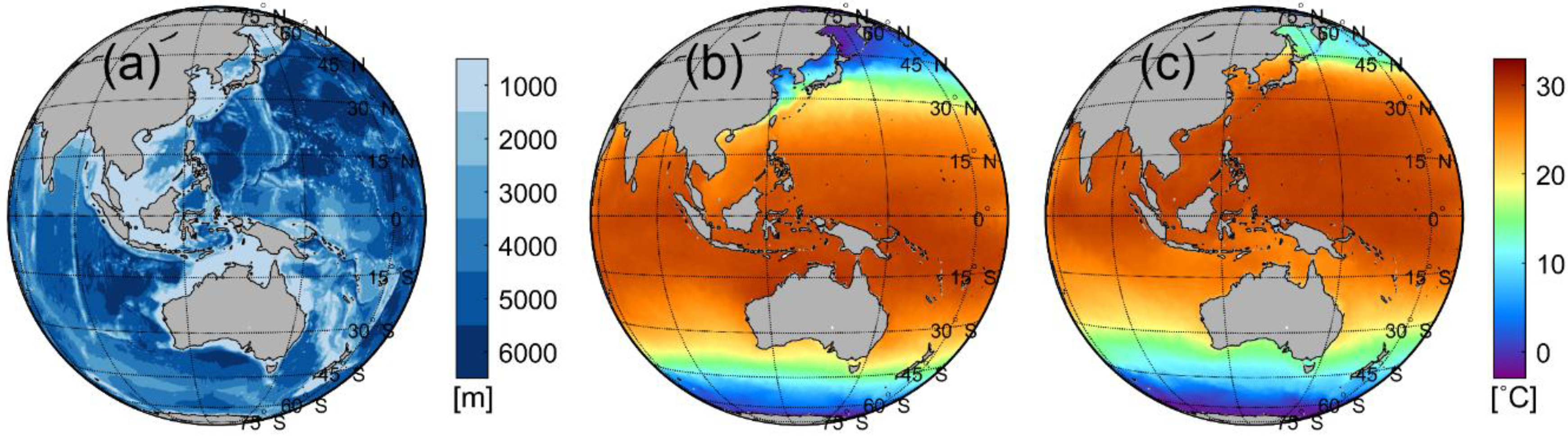
2.1. Satellite Data
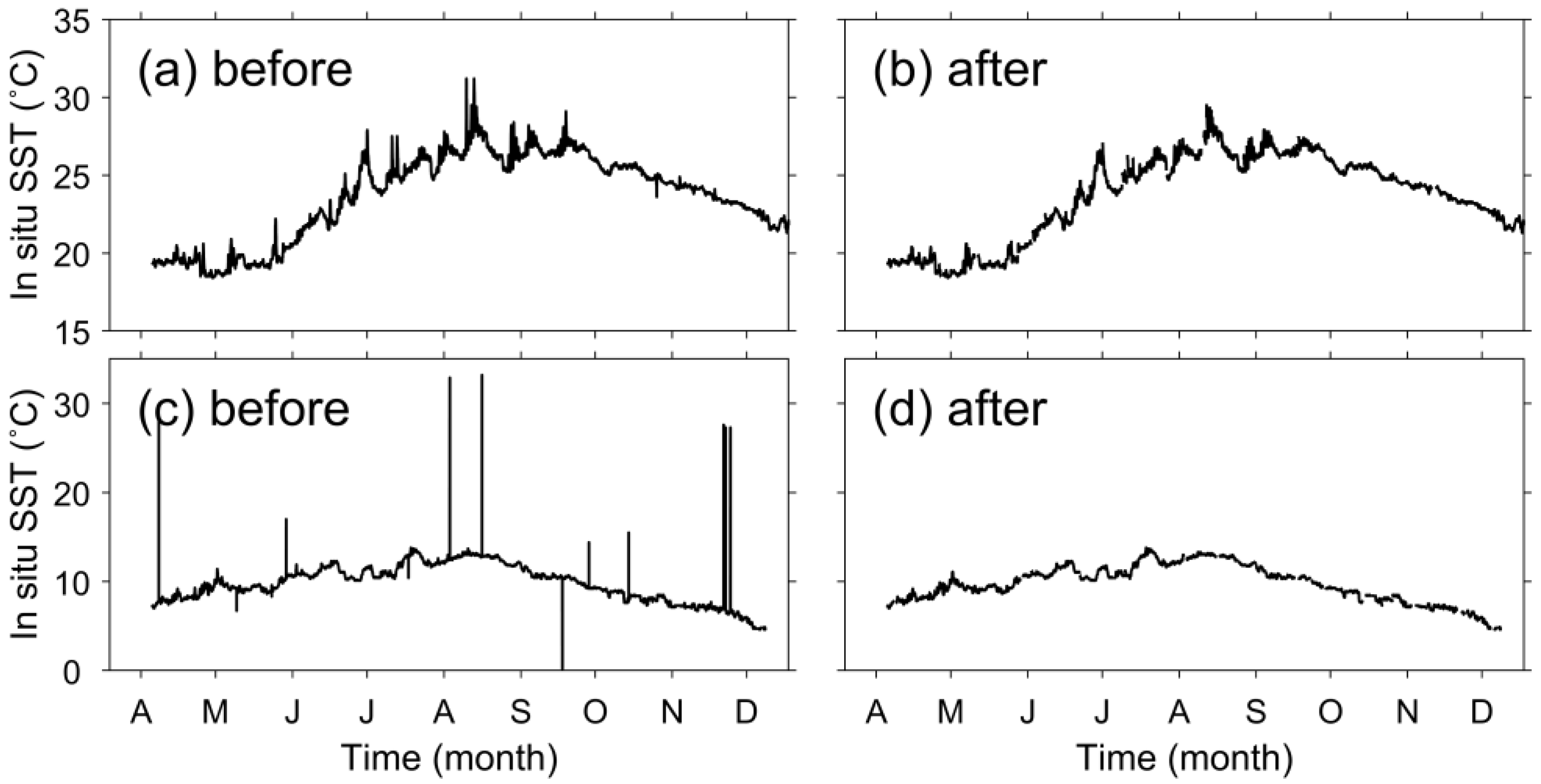
2.2. In Situ Temperature Measurements
2.3. Sea Surface Wind
2.4. Daily Sea Surface Temperature
3. Methods
3.1. Removal of Cloud Contaminated and Problematic Pixels
3.2. Sea Surface Temperature Retrieval Equations
3.3. Collocation Procedure and Validation
3.4. Regression Method
4. Results
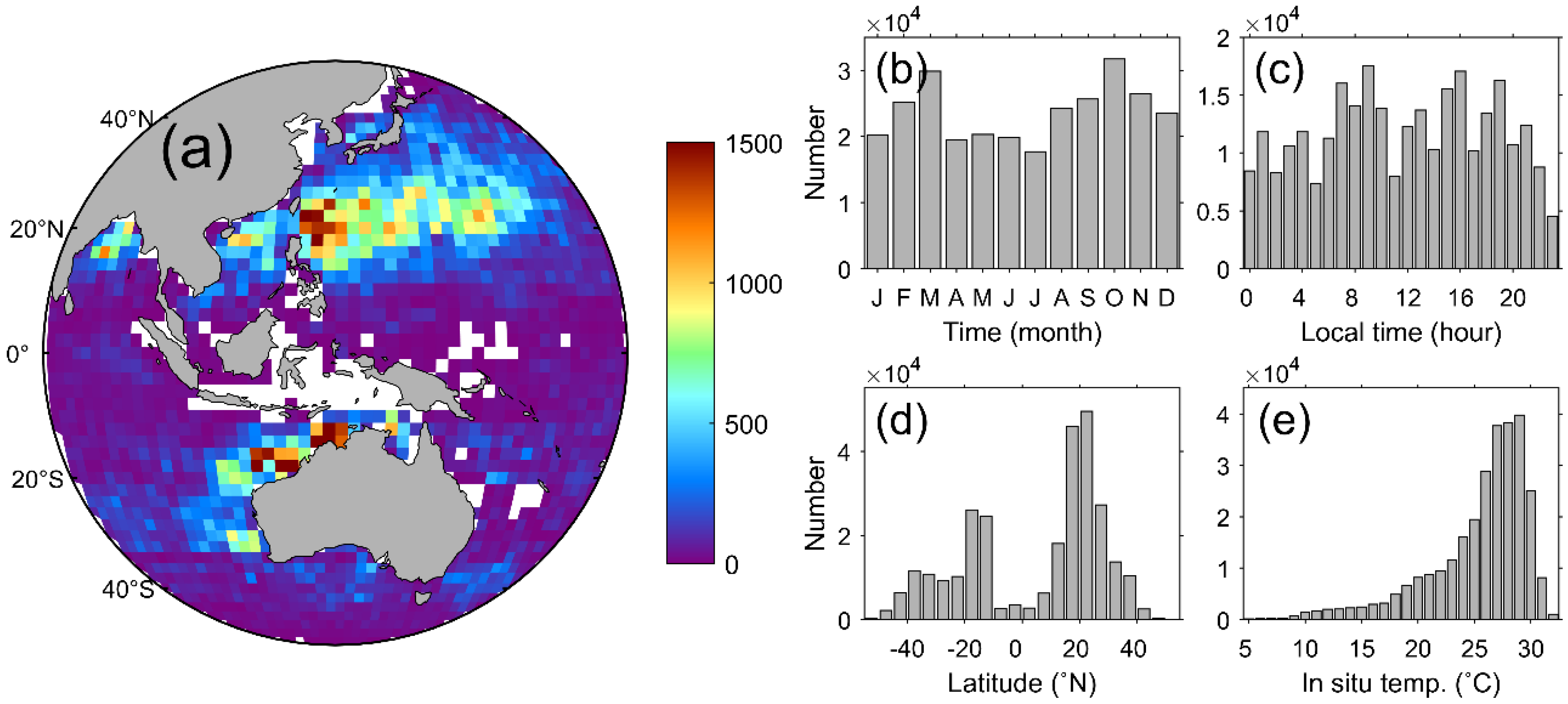
4.1. Characteristics of the Matchup Database
4.2. SST Coefficients of COMS/MI
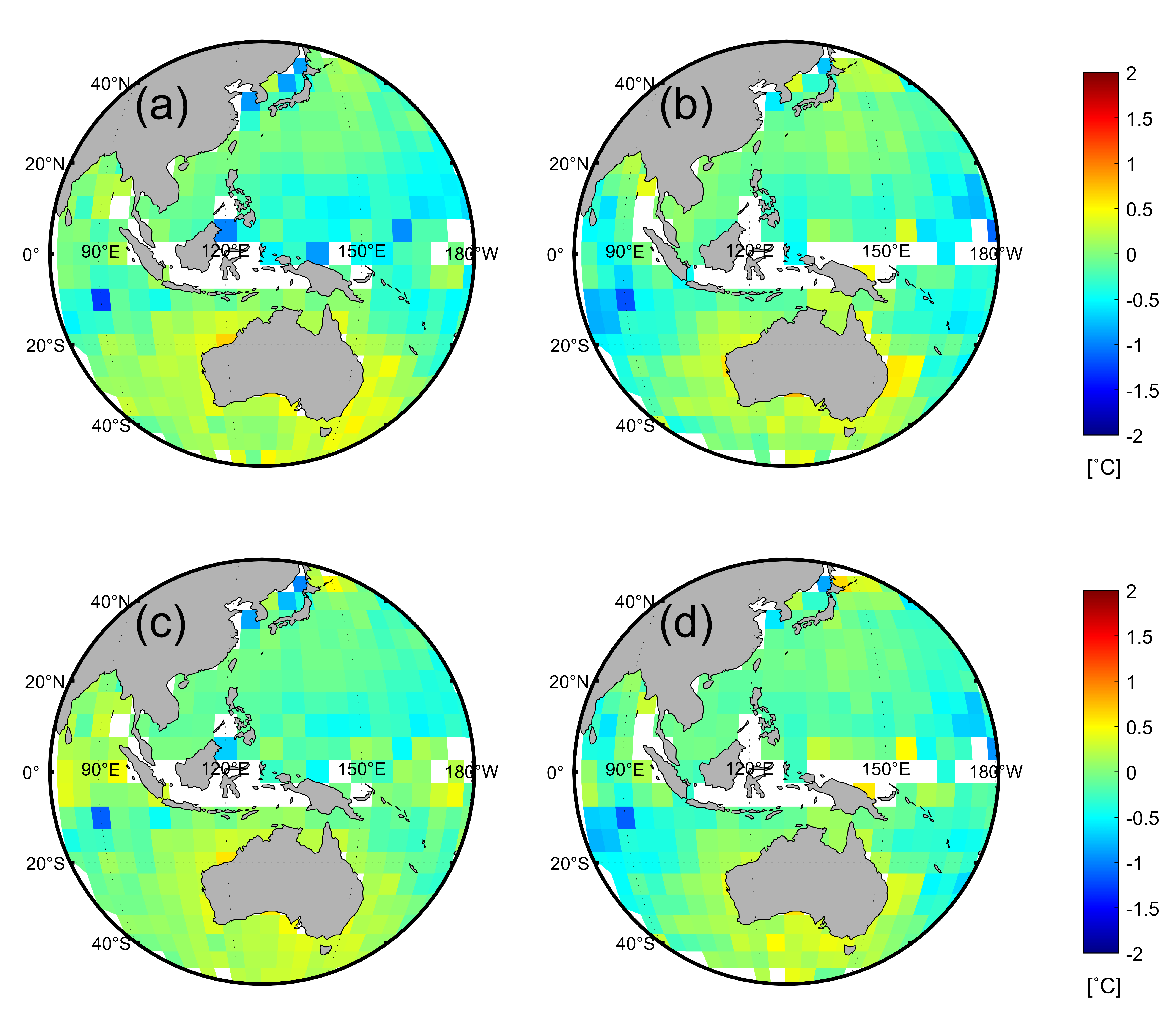
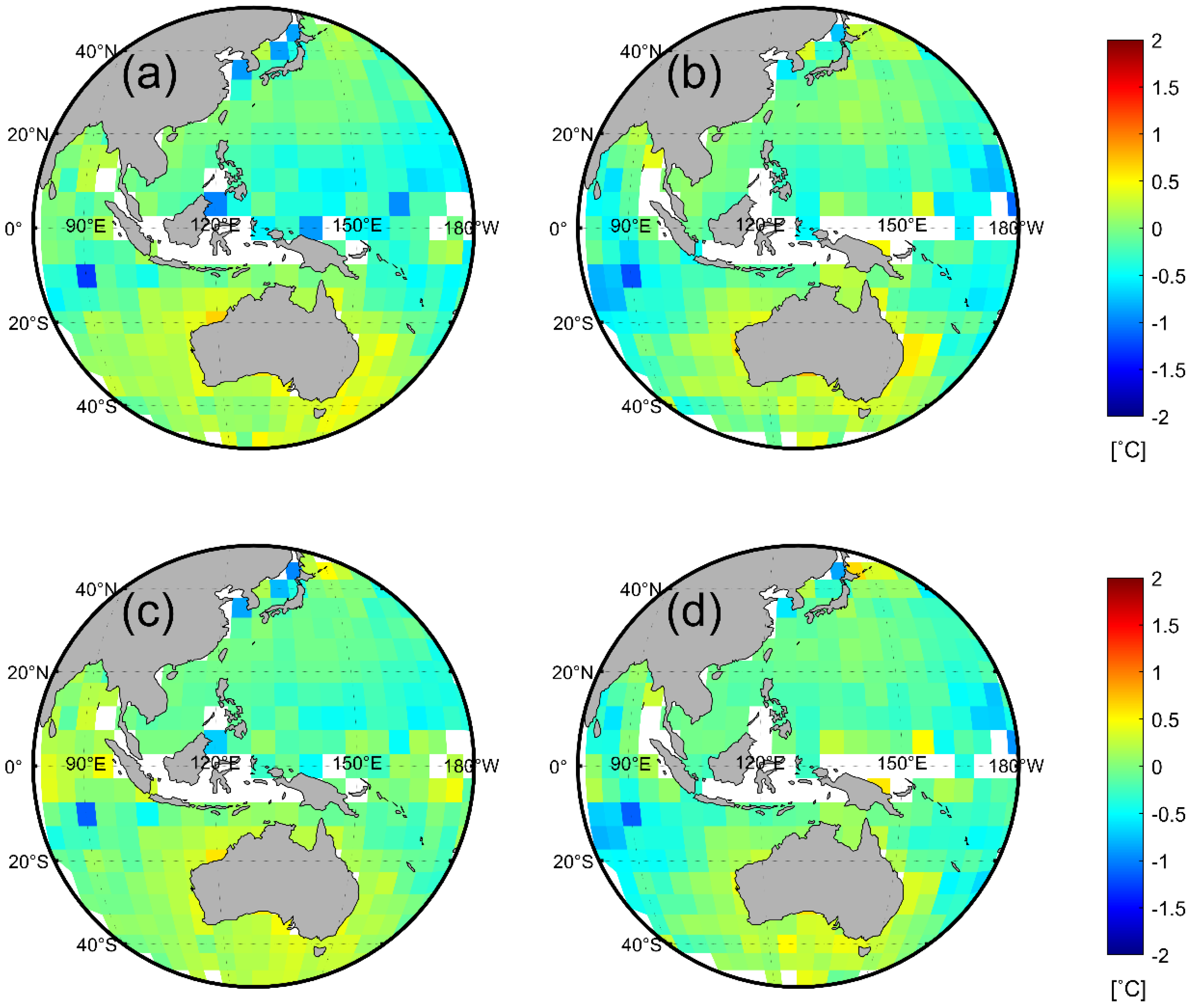
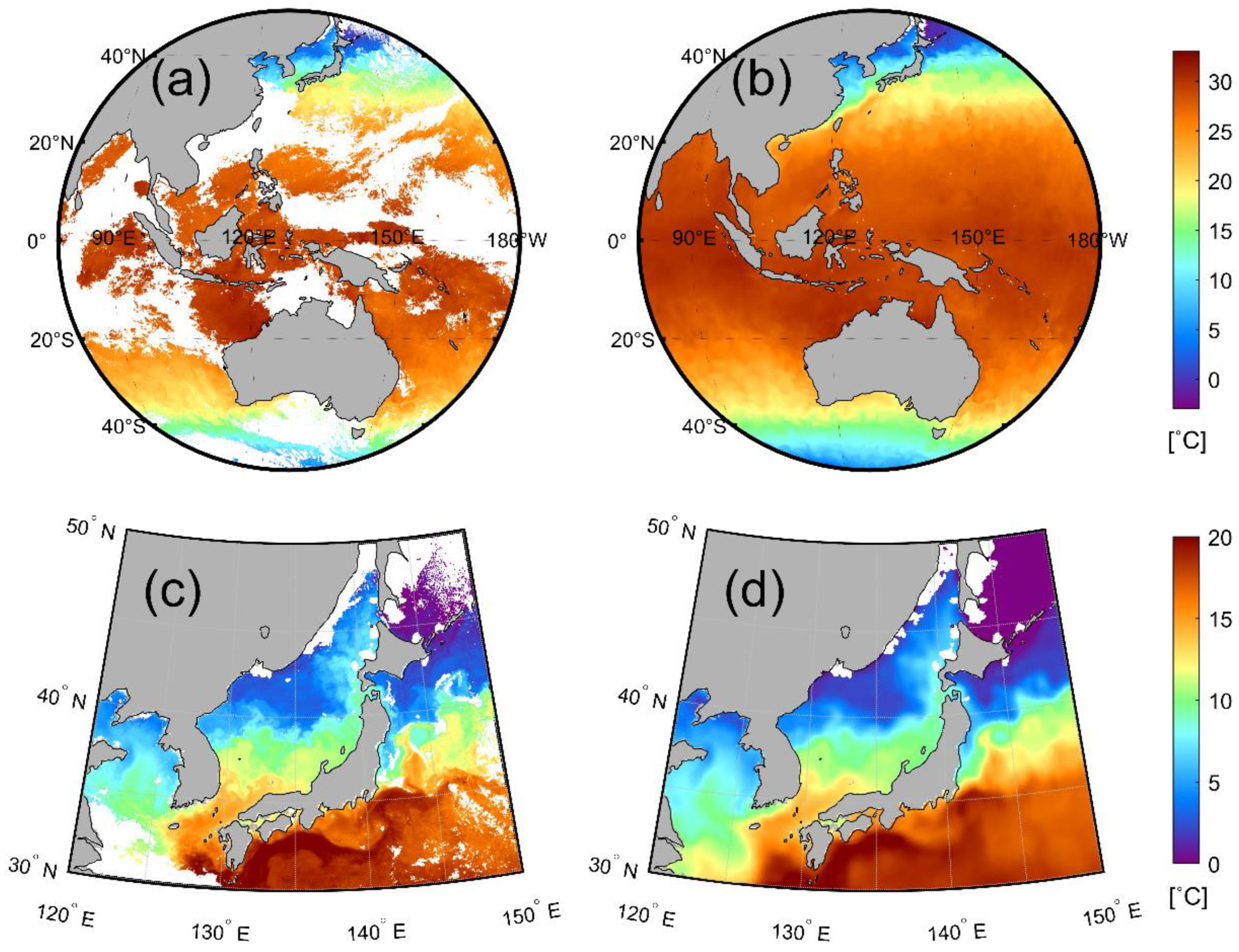
4.3. Accuracy of COMS/MI SST and Spatial Distribution of Errors
4.4. Characteristics of Sea Surface Temperature Errors
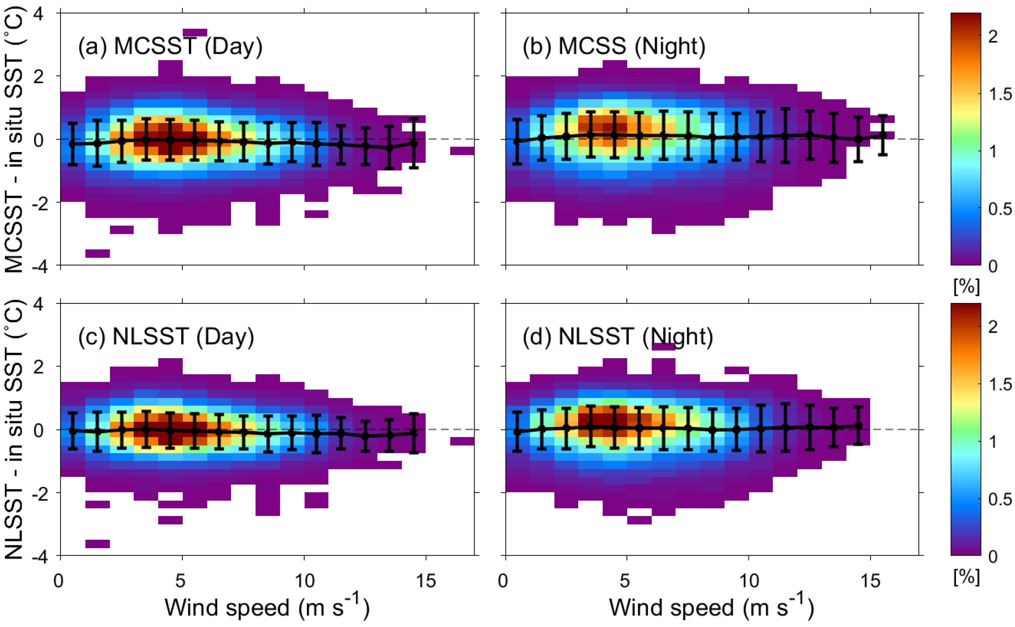
4.4.1. Dependence of SST Errors on Wind Speed
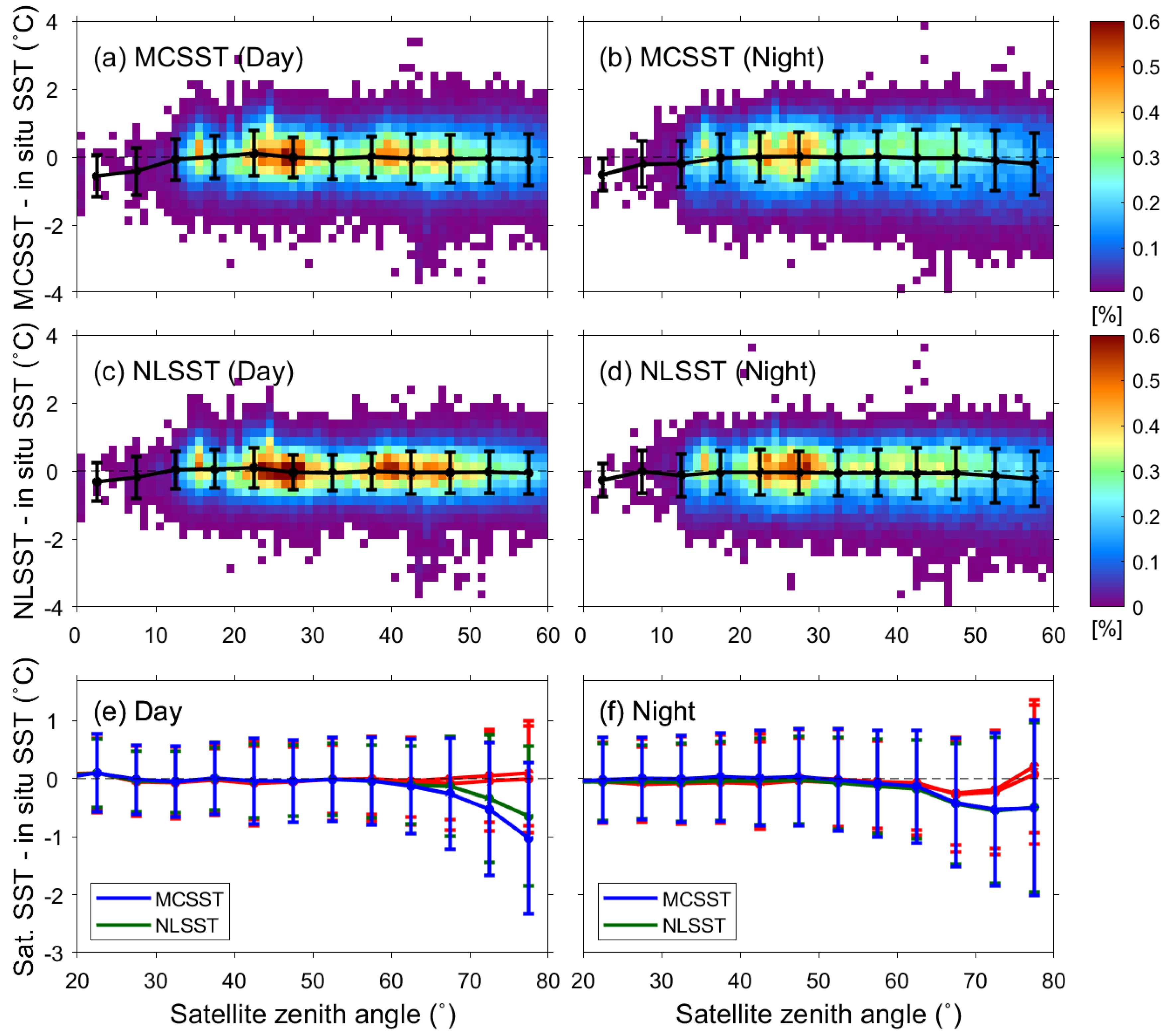
4.4.2. Effect of Satellite Zenith Angle
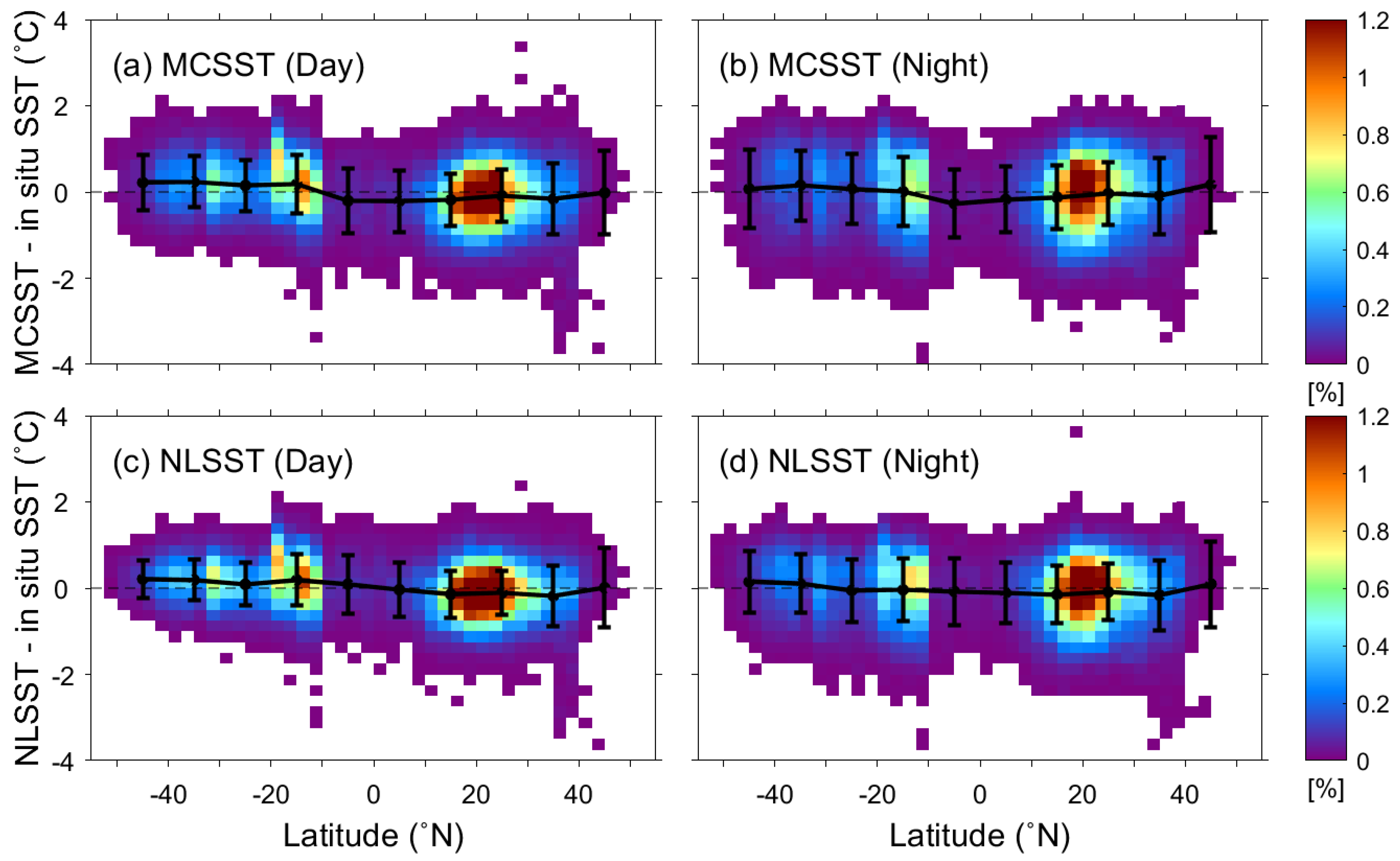
4.4.3. Latitudinal Distribution of SST Errors
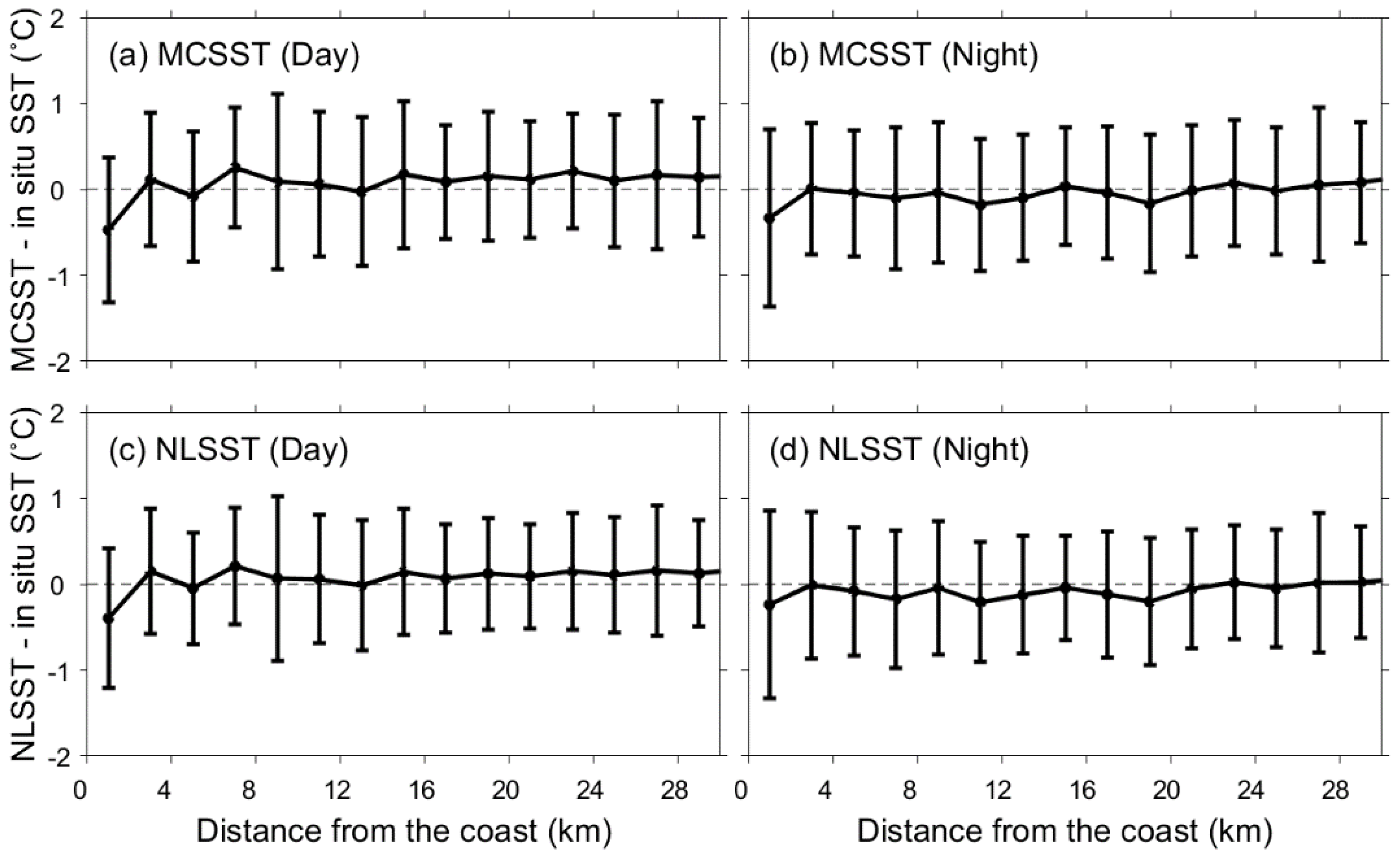
4.4.4. Coastal Effects on SST Errors
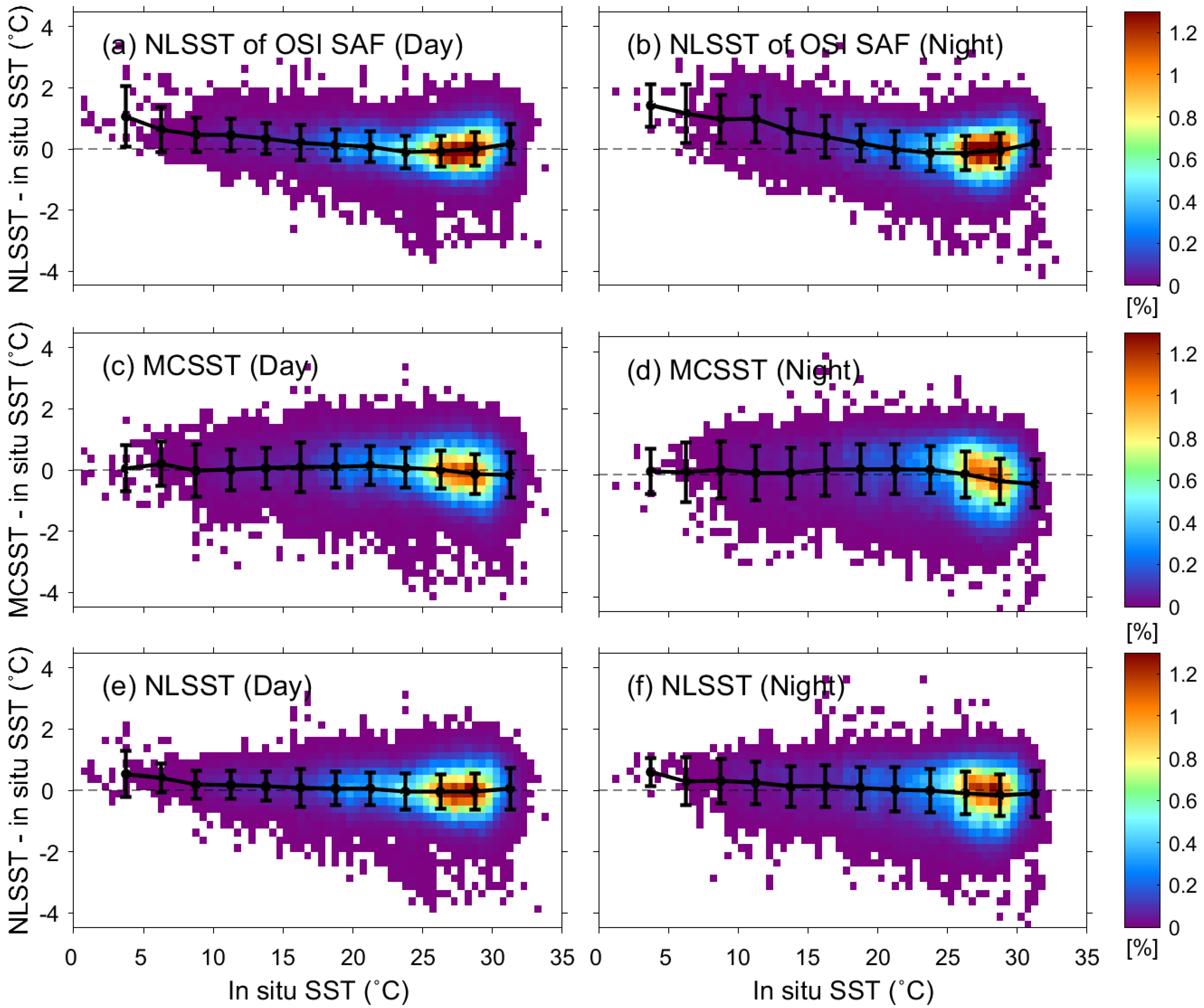
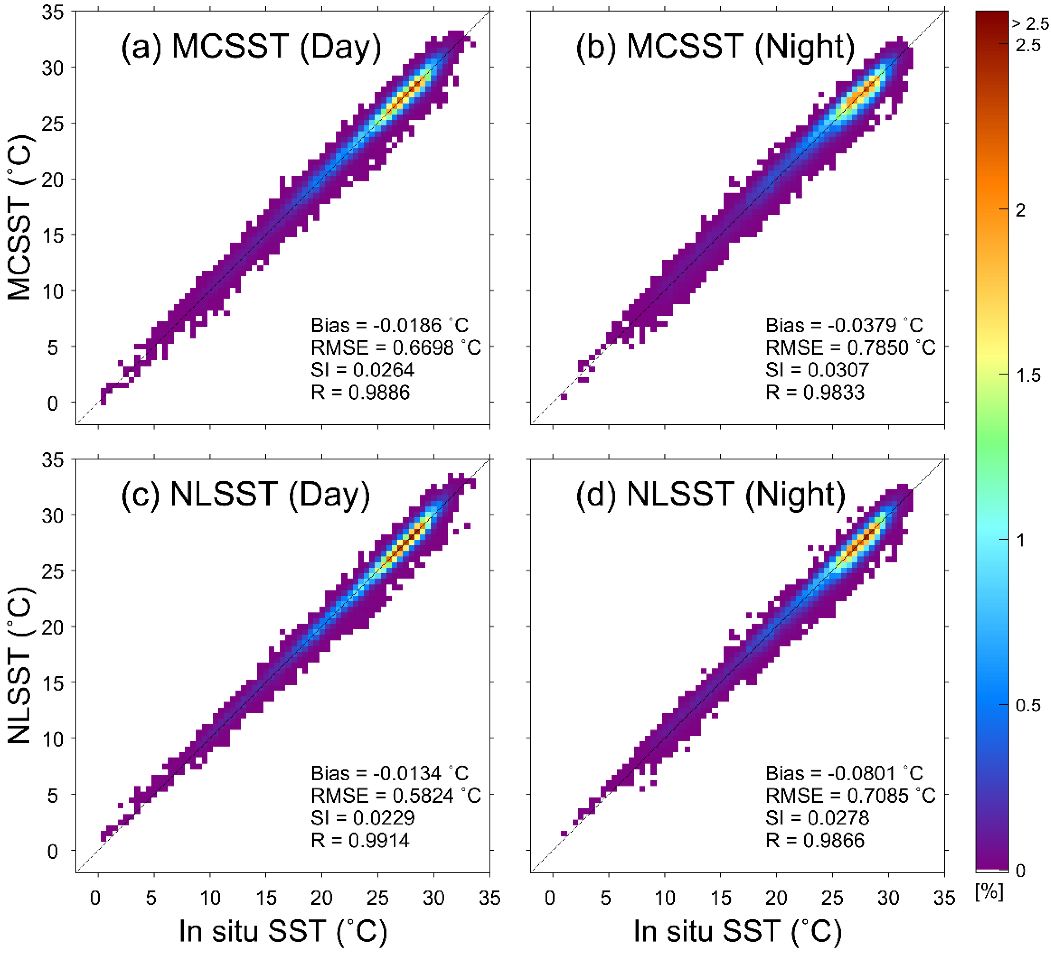
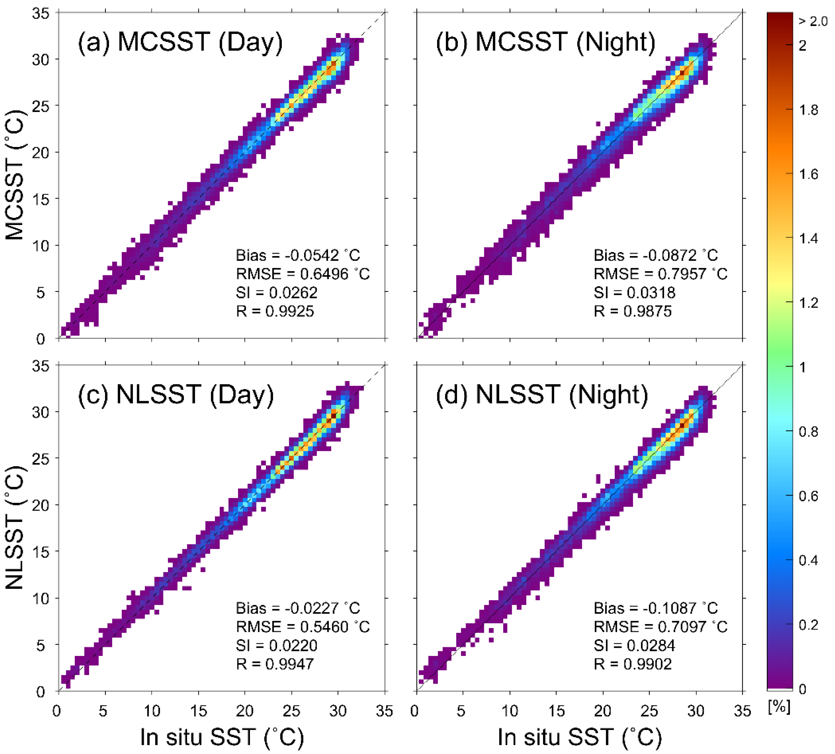
4.5. Validation of Retrieved SST
4.6. Comparison of Derived SSTs with Other SST Product
5. Discussion
6. Summary and Conclusions
Author Contributions
Funding
Acknowledgments
Conflicts of Interest
References
- Zhang, F.; Li, X.; Hu, J.; Sun, Z.; Zhu, J.; Liu, Z.; Chen, Z. Summertime sea surface temperature and salinity fronts in the southern Taiwan Strait. Int. J. Remote Sens. 2014, 35, 4452–4466. [Google Scholar] [CrossRef]
- Li, X.; Donato, T.; Zheng, Q.; Pichel, W.G.; Clemente-Colon, P. An extraordinary breach of the Gulf Stream north wall by a cold water intrusion. Geophys. Res. Lett. 2002, 29. [Google Scholar] [CrossRef]
- Li, X.; Zheng, W.; Pichel, W.G.; Zou, C.; Clemente-Colon, P.; Friedman, K.S. A cloud line over the Gulf Stream. Geophys. Res. Lett. 2004, 31, L14108. [Google Scholar] [CrossRef]
- Kawai, Y.; Wada, A. Diurnal sea surface temperature variation and its impact on the atmosphere and ocean: A review. J. Oceanogr. 2007, 63, 721–744. [Google Scholar] [CrossRef]
- Casey, K.S.; Cornillon, P. Global and regional sea surface temperature trends. J. Clim. 2001, 14, 3801–3818. [Google Scholar] [CrossRef]
- Hartmann, D.L.; Klein Tank, A.M.G.; Rusticucci, M.; Alexander, L.V.; Brönnimann, S.; Charabi, Y.; Dentener, F.J.; Dlugokencky, E.J.; Easterling, D.R.; Kaplan, A.; et al. Observations: Atmosphere and surface. In Climate Change 2013: The Physical Science Basis. Contribution of Working Group I to the Fifth Assessment Report of the Intergovernmental Panel on Climate Change; Stocker, T.F., Qin, D., Plattner, G.-K., Tignor, M., Allen, S.K., Boschung, J., Nauels, A., Xia, Y., Bex, V., Midgley, P.M., Eds.; Cambridge University Press: Cambridge, UK; New York, NY, USA, 2013; pp. 1–96. [Google Scholar]
- Maturi, E.; Harris, A.; Mittaz, J.; Merchant, C.; Potash, B.; Meng, W.; Sapper, J. NOAA’s sea surface temperature products from operational geostationary satellites. Bull. Am. Meteorol. Soc. 2008, 89, 1877–1888. [Google Scholar] [CrossRef]
- Schmetz, J.; Pili Tjemkes, P.S.; Just, D.; Kerkmann, J.; Rota, S.; Ratier, A. An introduction to Meteosat Second Generation (MSG). Bull. Am. Meteorol. Soc. 2002, 83, 977–992. [Google Scholar] [CrossRef]
- Bessho, K.; Date, K.; Hayashi, M.; Ikeda, A.; Imai, T.; Inoue, H.; Kumagai, Y.; Miyakawa, T.; Murata, H.; Ohno, T.; et al. An Introduction to Himawari-8/9-Japan’s new-generation geostationary meteorological satellites. J. Meteorol. Soc. Jpn. 2016, 94, 151–183. [Google Scholar] [CrossRef]
- Anding, D.; Kauth, R. Estimation of sea surface temperature from space. Remote Sens. Environ. 1970, 1, 217–220. [Google Scholar] [CrossRef]
- Prabhakara, C.; Dalu, G.; Kunde, V.G. Estimation of sea surface temperature from remote sensing in 11 to 13 µm window region. J. Geophys. Res. 1974, 79, 5039–5044. [Google Scholar] [CrossRef]
- McMillin, L.M. Estimation of sea surface temperature from two infrared window measurements with different absorptions. J. Geophys. Res. 1975, 80, 5113–5117. [Google Scholar] [CrossRef]
- Bernstein, R.L. Sea surface temperature estimation using the NOAA-6 satellite Advanced Very High Resolution Radiometer. J. Geophys. Res. 1982, 87, 9455–9465. [Google Scholar] [CrossRef]
- McMillin, L.M.; Crosby, D.S. Theory and validation of the multiple window sea surface temperature technique. J. Geophys. Res. 1984, 89, 3655–3661. [Google Scholar] [CrossRef]
- McClain, E.P.; Pichel, W.G.; Walton, C.C. Comparative performance of Avhrr-based Multichannel Sea Surface Temperatures. J. Geophys. Res. 1985, 90, 11587–11601. [Google Scholar] [CrossRef]
- Walton, C.C. Nonlinear multichannel algorithms for estimating sea surface temperature with AVHRR Satellite Data. J. Appl. Meteorol. 1988, 27, 115–124. [Google Scholar] [CrossRef]
- Walton, C.C.; Pichel, W.G.; Sapper, J.F.; May, D.A. The development and operational application of nonlinear algorithms for the measurement of sea surface temperatures with the NOAA polar-orbiting environmental satellites. J. Geophys. Res. 1998, 103, 27999–28012. [Google Scholar] [CrossRef]
- Kilpatrick, K.A.; Podestá, G.P.; Evans, R. Overview of the NOAA/NASA advanced very high resolution radiometer Pathfinder algorithm for sea surface temperature and associated matchup database. J. Gephys. Res. 2001, 106, 9179–9197. [Google Scholar] [CrossRef]
- Li, X.; Pichel, W.; Maturi, E.; Clemente-Colón, P.; Sapper, J. Deriving the operational nonlinear multi-channel sea surface temperature algorithm coefficients for NOAA-15 AVHRR/3. Int. J. Remote Sens. 2001, 22, 699–704. [Google Scholar] [CrossRef]
- OSI SAF. Geostationary Sea Surface Temperature Product User Manual; Technical Report; EUMETSAT: Berlin, Germany, 2011. [Google Scholar]
- François, C.; Brisson, A.; Le Borgne, P.; Marsouin, A. Definition of a radiosounding database for sea surface brightness temperature simulations: Application to sea surface temperature retrieval algorithm determination. Remote Sens. Environ. 2002, 81, 309–326. [Google Scholar] [CrossRef]
- Petrenko, B.; Ignatov, A.; Kihai, Y.; Stroup, J.; Dash, P. Evaluation and selection of SST regression algorithms for JPSS VIIRS. J. Geophys. Res. Atmos. 2014, 119, 4580–4599. [Google Scholar] [CrossRef]
- Kramar, M.; Ignatov, A.; Petrenko, B.; Kihai, Y.; Dash, P. Near Real Time SST Retrievals from Himawari-8 at NOAA using ACSPO system. In Proceedings of the Ocean Sensing and Monitoring VIII, Baltimore, MD, USA, 17–21 April 2016; Arnone, R.A., Hou, W.W., Eds.; SPIE: Baltimore, MD, USA, 2016; p. 98270L. [Google Scholar] [CrossRef]
- Liang, X.; Ignatov, A.; Kihai, Y. Implementation of the Community Radiative Transfer Model in Advanced Clear-Sky Processor for Oceans and validation against nighttime AVHRR radiances. J. Geophys. Res. 2009, 114, D06112. [Google Scholar] [CrossRef]
- Dash, P.; Ignatov, A. Validation of clear-sky radiances over oceans simulated with MODTRAN4. 2 and global NCEP GDAS fields against nighttime NOAA15-18 and MetOp-A AVHRR data. Remote Sens. Environ. 2008, 112, 3012–3029. [Google Scholar] [CrossRef]
- Merchant, C.J.; Le Borgne, P.; Marsouin, A.; Roquet, H. Optimal estimation of sea surface temperature from split-window observations. Remote Sens. Environ. 2008, 112, 2469–2484. [Google Scholar] [CrossRef]
- Kurihara, Y.; Murakami, H.; Kachi, M. Sea surface temperature from the new Japanese geostationary meteorological Himawari-8 satellite. Geophys. Res. Lett. 2016, 43, 1234–1240. [Google Scholar] [CrossRef]
- Koner, P.K.; Harris, A.R.; Maturi, E. A physical deterministic inverse method for operational satellite remote sensing: An application for sea surface temperature retrievals. IEEE Trans. Geosci. Remote Sens. 2015, 53, 5872–5888. [Google Scholar] [CrossRef]
- McPhaden, M.J.; Picaut, J. El Nino-Southern Oscillation displacements of the western equatorial Pacific warm pool. Science 1990, 250, 1385–1388. [Google Scholar] [CrossRef] [PubMed]
- Qu, T. Mixed layer heat balance in the western North Pacific. J. Geophys. Res. 2003, 108, 3242. [Google Scholar] [CrossRef]
- Kim, D.; Ahn, M.-H.; Choi, M. Inter-comparison of the infrared channels of the Meteorological Imager onboard COMS and hyperspectral IASI data. Adv. Atmos. Sci. 2015, 32, 979–990. [Google Scholar] [CrossRef]
- Goldberg, M.; Ohring, G.; Butler, J.; Cao, C.; Datla, R.; Doelling, D.V.; Hewison, G.T.; Iacovazzi, B.; Kim, D.; Kurino, T.; et al. The global space-based inter-calibration system. Bull. Am. Meteorol. Soc. 2011, 92, 467–475. [Google Scholar] [CrossRef]
- National Meteorological Satellite Center. Available online: http://nmsc.kma.go.kr (accessed on 8 October 2018).
- Lumpkin, R.; Pazos, M. Measuring surface currents with SVP drifters: The instrument, its data and some results. In Lagrangian Analysis and Prediction of Coastal and Ocean Dynamics; Griffa, A., Kirwan, J.A.D., Eds.; Cambridge University Press: Cambridge, UK, 2007; pp. 39–67. [Google Scholar]
- Xu, F.; Ignatov, A. In situ SST Quality Monitor (iQUAM). J. Atmos. Ocean. Technol. 2014, 31, 164–180. [Google Scholar] [CrossRef]
- O’Carroll, A.G.; Eyre, J.R.; Saunders, R.W. Three-way error analysis between AATSR, AMSR-E, and in situ sea surface temperature observations. J. Atmos. Ocean. Technol. 2008, 25, 1197–1207. [Google Scholar] [CrossRef]
- Gentemann, C.L.; Minnett, P.J. Radiometric measurements of ocean surface thermal variability. J. Geophys. Res. 2008, 113, C08017. [Google Scholar] [CrossRef]
- Gentemann, C.L. Three way validation of MODIS and AMSR-E sea surface temperatures. J. Geophys. Res. 2014, 119, 2583–2598. [Google Scholar] [CrossRef]
- Donlon, C.J.; Minnett, P.J.; Gentemann, C.; Nightingale, T.J.; Barton, I.J.; Ward, B.; Murray, J. Toward improved validation of satellite sea surface skin temperature measurements for climate research. J. Clim. 2002, 15, 353–369. [Google Scholar] [CrossRef]
- Remote Sensing Systems. Available online: http://www.remss.com (accessed on 8 October 2018).
- Hosoda, K.; Murakami, H.; Sakaida, F.; Kawamura, H. Algorithm and validation of sea surface temperature observation using MODIS sensors aboard Terra and Aqua in the Western North Pacific. J. Oceanogr. 2007, 63, 267–280. [Google Scholar] [CrossRef]
- Martin, M.J.; Hines, A.; Bell, M.J. Data assimilation in the FOAM operational short-range ocean forecasting system: A description of the scheme and its impact. Q. J. R. Meteorol. Soc. 2007, 133, 981–995. [Google Scholar] [CrossRef]
- Donlon, C.J.; Martin, M.; Stark, J.; Roberts-Jones, J.; Fiedler, E.; Wimmer, W. The Operational Sea Surface Temperature and Sea Ice Analysis (OSTIA) system. Remote Sens. Environ. 2012, 116, 140–158. [Google Scholar] [CrossRef]
- Copernicus Marine Environment Monitoring Service. Available online: http://marine.copernicus.eu (accessed on 8 October 2018).
- Saunders, R.W.; Kriebel, K.T. An improved method for detecting clear sky and cloudy radiances from AVHRR data. Int. J. Remote Sens. 1988, 9, 123–150. [Google Scholar] [CrossRef]
- Stowe, L.L.; McClain, E.P.; Carey, R.; Pellegrino, P.; Gutman, G.G.; Davis, P.; Long, C.; Hart, S. Global distribution of cloud cover derived from NOAA/AVHRR operational satellite data. Adv. Space Res. 1991, 3, 51–54. [Google Scholar] [CrossRef]
- Závody, A.M.; Mutlow, C.T.; Llewellyn-Jones, D.T. Cloud clearing over the ocean in the processing of data from the Along-Track Scanning Radiometer (ATSR). J. Atmos. Ocean. Technol. 2000, 17, 595–615. [Google Scholar] [CrossRef]
- Wick, G.A.; Bates, J.J.; Scott, D.J. Satellite and skin layer effects on the accuracy of sea surface temperature measurements from the GOES satellite. J. Atmos. Ocean. Technol. 2002, 19, 1834–1848. [Google Scholar] [CrossRef]
- Park, K.; Lee, E.; Li, X.; Chung, S.; Sohn, E.; Lee, E.; Li, X.; Chung, S.; Sohn, E. NOAA/AVHRR sea surface temperature accuracy in the East/Japan Sea. Int. J. Digit. Earth 2015, 8, 784–804. [Google Scholar] [CrossRef]
- Petrenko, B.; Ignatov, A.; Kihai, Y.; Heidinger, A. Clear-sky mask for the advanced clear-sky processor for oceans. J. Atmos. Ocean. Technol. 2010, 27, 1609–1623. [Google Scholar] [CrossRef]
- Cayula, J.-F.P.; May, D.A.; McKenzie, B.D.; Willis, K.D. Viirs-derived sst at the naval oceanographic office: From evaluation to operation. Ocean Sens. Monit. 2013, 8724. [Google Scholar] [CrossRef]
- McBride, W.; Arnone, B.A.; Cayula, J. Improvements of satellite SST retrievals at full swath. In Proceedings of the Ocean Sensing and Monitoring V, Baltimore, MD, USA, 26 April–1 May 2013; Hou, W.W., Arnone, R.A., Eds.; SPIE: Baltimore, MD, USA, 2013; p. 87240R. [Google Scholar] [CrossRef]
- Marsouin, A.; Le Borgne, P.; Legendre, G.; Péré, S.; Roquet, H. Six years of OSI-SAF METOP-A AVHRR sea surface temperature. Remote Sens. Environ. 2015, 159, 288–306. [Google Scholar] [CrossRef]
- Huber, P.J.S. Robust estimation of a location parameter. Ann. Math. Stat. 1964, 35, 73–101. [Google Scholar] [CrossRef]
- Holland, P.W.; Welsch, R.E. Robust regression using iteratively reweighted least-squares. Commun. Stat. Theory Methods 1977, 6, 813–827. [Google Scholar] [CrossRef]
- Rousseeuw, P.J.; Leroy, A.M. Robust Regression and Outlier Detection; John Wiley & Sons, Inc.: New York, NY, USA, 1987. [Google Scholar]
- Andersen, R. Modern Methods for Robust Regression. Quantitative Applications in the Social Sciences; Sage Publications: Los Angeles, CA, USA, 2008. [Google Scholar]
- Wilcox, R.R. Introduction to Robust Estimation and Hypothesis Testing, 3rd ed.; Academic Press: San Diego, CA, USA, 2012. [Google Scholar]
- Soukissian, T.H.; Karathanasi, F.E. On the use of robust regression methods in wind speed assessment. Renew. Energy 2016, 99, 1287–1298. [Google Scholar] [CrossRef]
- Simpson, J.J.; Humphrey, C. An automated cloud screening algorithm for daytime AVHRR imagery. J. Geophys. Res. 1990, 95, 13459–13481. [Google Scholar] [CrossRef]
- Li, X.; Pichel, W.; Clemente-Colón, P.; Krasnopolsky, V.; Sapper, J. Validation of coastal sea and lake surface temperature measurements derived from NOAA/AVHRR data. Int. J. Remote Sens. 2001, 22, 1285–1303. [Google Scholar] [CrossRef]
- Kawamura, H.; Qin, H.; Sakaida, F.; Setiawan, R.Y. Hourly sea surface temperature retrieval using the Japanese geostationary satellite, multi-functional transport satellite (MTSAT). J. Oceanogr. 2010, 66, 61–70. [Google Scholar] [CrossRef]
- Donlon, C.J.; Nightingale, T.J.; Sheasby, T.; Turner, J.; Robinson, I.S.; Emergy, W.J. Implications of the oceanic thermal skin temperature deviation at high wind speed. Geophys. Res. Lett. 1999, 26, 2505–2508. [Google Scholar] [CrossRef]
- Minnett, P.J. Radiometric measurements of the sea-surface skin temperature: The competing roles of the diurnal thermocline and the cool skin. Int. J. Remote Sens. 2003, 24, 5033–5047. [Google Scholar] [CrossRef]
- Donlon, C.; Rayner, N.; Robinson, I.; Poulter, D.J.S.; Casey, K.S.; Vazquez-Cuervo, J.; Armstrong, E.; Bingham, A.; Arino, O.; Gentemann, C.; et al. The global ocean data assimilation experiment high-resolution sea surface temperature pilot project. Bull. Am. Meteorol. Soc. 2007, 88, 1197–1213. [Google Scholar] [CrossRef]
- Merchant, C.J.; Harris, A.R.; Roquet, H.; Le Borgne, P. Retrieval characteristics of non-linear sea surface temperature from the Advanced very High Resolution Radiometer. Geophys. Res. Lett. 2009, 36, L17604. [Google Scholar] [CrossRef]
- Ricciardulli, L.; Wentz, L.J. Uncertainties in sea surface temperature retrievals from space: Comparison of microwave and infrared observations from TRMM. J. Geophys. Res. 2004, 109. [Google Scholar] [CrossRef]
- Castro, S.L.; Wick, G.A.; Emery, W.J. Evaluation of the relative performance of sea surface temperature measurements from different types of drifting and moored buoys using satellite-derived reference products. J. Geophys. Res. 2012, 117. [Google Scholar] [CrossRef]
- Reynolds, R.W.; Smith, T.M.; Liu, C.; Chelton, D.B.; Casey, K.S.; Schlax, M.G. Daily high-resolution-blended analyses for sea surface temperature. J. Clim. 2007, 20, 5473–5496. [Google Scholar] [CrossRef]
- Reynolds, R.W.; Chelton, D.B. Comparisons of daily sea surface temperature analyses for 2007–08. J. Clim. 2010, 23, 3545–3562. [Google Scholar] [CrossRef]


| Channel | Description | Wavelength (μm) | Bandwidth (μm) | NEDT at 300K (K) | Spatial Resolution (km) |
|---|---|---|---|---|---|
| 1 | VIS | 0.675 | 0.55–0.80 | 1 | |
| 2 | SWIR | 3.75 | 3.5–4.0 | <0.10 | 4 |
| 3 | WV | 6.75 | 6.5–7.0 | <0.12 | 4 |
| 4 | IR1 | 10.8 | 10.3–11.3 | <0.12 | 4 |
| 5 | IR2 | 12.0 | 11.5–12.5 | <0.20 | 4 |
| Criteria | Thresholds | |
|---|---|---|
| Day | Night | |
| VIS | >5% | - |
| BTIR1 | <−3.5 °C | <−3.5 °C |
| STD VIS | >0.5% | - |
| STD BTIR1 | >0.7 °C | >0.5 °C |
| STD BTIR2 | >0.7 °C | >0.5 °C |
| Max. VIS–Min. VIS | >3% | - |
| Max. BTIR1–Min. BTIR1 | >0.7 °C | >0.5 °C |
| Max. BTIR2–Min. BTIR2 | >0.7 °C | >0.5 °C |
| BTIR1–BTIR2 | >0.0032 * BTIR12 + 0.0996 * BTIR1 + 1.607 (°C) (if BTIR1 ≤ 20 °C) >6 °C (if BTIR1 > 20 °C) | |
| BTSWIR–BTIR2 | - | <exp(−9.375 + 0.0342 * BTIR1) (°C) |
| BTIR1–Max. BTIR1 for 10 day | <−3 °C | <−3 °C |
| SZA | >60° | >60° |
| SRA | <15° | - |
| |SST–FGSST| | >3 °C | >3 °C |
| Alg. | Time | Equation | Ref. | RMSE (°C) | Bias (°C) |
|---|---|---|---|---|---|
| MCSST | Night | [50] | 0.55 | −0.01 | |
| NLSST | Day | [50] | 0.58 | −0.01 | |
| Day | [51] | 0.55 | 0.01 | ||
| Night | 0.52 | −0.04 | |||
| All | [18] | 0.58 | −0.01 | ||
| 0.71 | −0.08 | ||||
| All | [52] | 0.34 | −0.01 | ||
| 0.29 | 0.00 | ||||
| All | [20] | 0.55 | 0.01 | ||
| 0.63 | −0.02 |
| Algorithm | Type | Time | Coefficients | RMSE (°C) | Bias (°C) | |||
|---|---|---|---|---|---|---|---|---|
| a0 | a1 | a2 | a3 | |||||
| MCSST | Split | Day | −0.4907 | 1.0039 | 1.9956 | 0.7340 | 0.67 | −0.02 |
| Split | Night | 0.6351 | 1.0196 | 1.5888 | 0.7250 | 0.79 | −0.04 | |
| Triple | Night | 2.0183 | 0.9849 | 0.7737 | 0.4149 | 0.56 | −0.02 | |
| NLSST | Split | Day | 2.1785 | 0.9071 | 0.0650 | 0.7499 | 0.58 | −0.01 |
| Split | Night | 2.7423 | 0.9272 | 0.0563 | 0.6946 | 0.71 | −0.08 | |
| Triple | Night | 3.2185 | 0.9381 | 0.0259 | 0.4450 | 0.52 | −0.04 | |
© 2018 by the authors. Licensee MDPI, Basel, Switzerland. This article is an open access article distributed under the terms and conditions of the Creative Commons Attribution (CC BY) license (http://creativecommons.org/licenses/by/4.0/).
Share and Cite
Woo, H.-J.; Park, K.-A.; Li, X.; Lee, E.-Y. Sea Surface Temperature Retrieval from the First Korean Geostationary Satellite COMS Data: Validation and Error Assessment. Remote Sens. 2018, 10, 1916. https://doi.org/10.3390/rs10121916
Woo H-J, Park K-A, Li X, Lee E-Y. Sea Surface Temperature Retrieval from the First Korean Geostationary Satellite COMS Data: Validation and Error Assessment. Remote Sensing. 2018; 10(12):1916. https://doi.org/10.3390/rs10121916
Chicago/Turabian StyleWoo, Hye-Jin, Kyung-Ae Park, Xiaofeng Li, and Eun-Young Lee. 2018. "Sea Surface Temperature Retrieval from the First Korean Geostationary Satellite COMS Data: Validation and Error Assessment" Remote Sensing 10, no. 12: 1916. https://doi.org/10.3390/rs10121916
APA StyleWoo, H.-J., Park, K.-A., Li, X., & Lee, E.-Y. (2018). Sea Surface Temperature Retrieval from the First Korean Geostationary Satellite COMS Data: Validation and Error Assessment. Remote Sensing, 10(12), 1916. https://doi.org/10.3390/rs10121916