Deep Memory Connected Neural Network for Optical Remote Sensing Image Restoration


Abstract
:1. Introduction
- We build a deep memory connected network for high-quality remote-sensing image restoration. Our network can handle various image restoration tasks such as super-resolution and Gaussian denoising at the same time. We can also achieve blind Gaussian denoising for unknown noise level. By simply changing training datasets, our network can be applicable for super-resolution with different upscale factors.
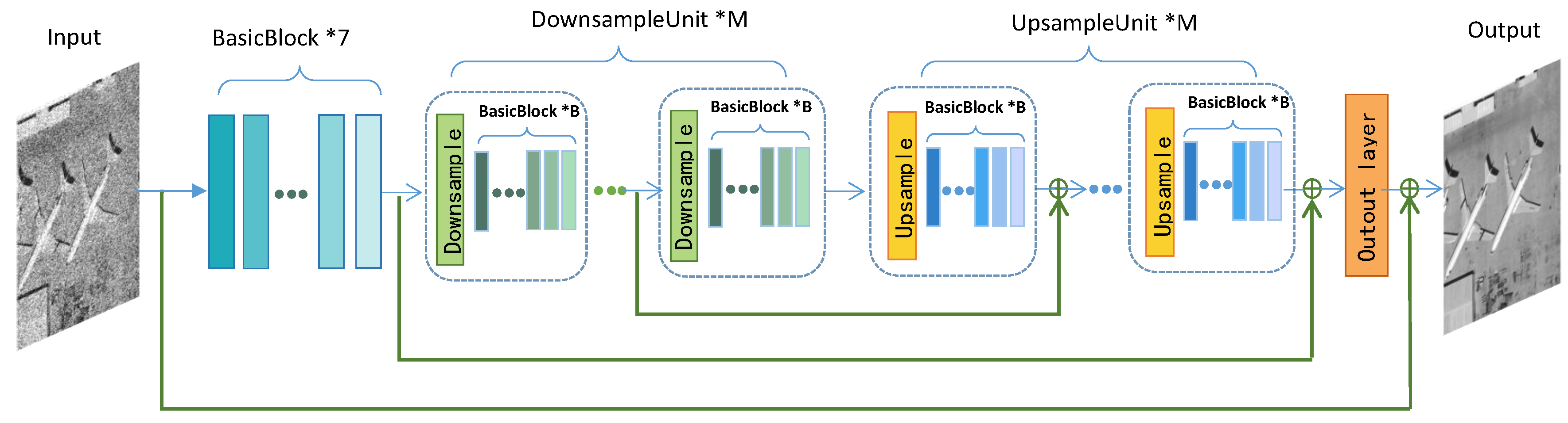
- Taking into account the lower layer information, DMCN is elaborately designed with local and global memory connections. With the global connection, DMCN only needs to predict high-frequency residual information instead of predicting the whole image. We use local residual in Basic Blocks to achieve fast error reduction.
- DMCN is elaborately designed with Downsample and Upsample Units to build an hourglass structure. With a Downsample Unit, we can shrink the spatial size of the feature map by 2, significantly reducing the memory footprint and time-consumption.
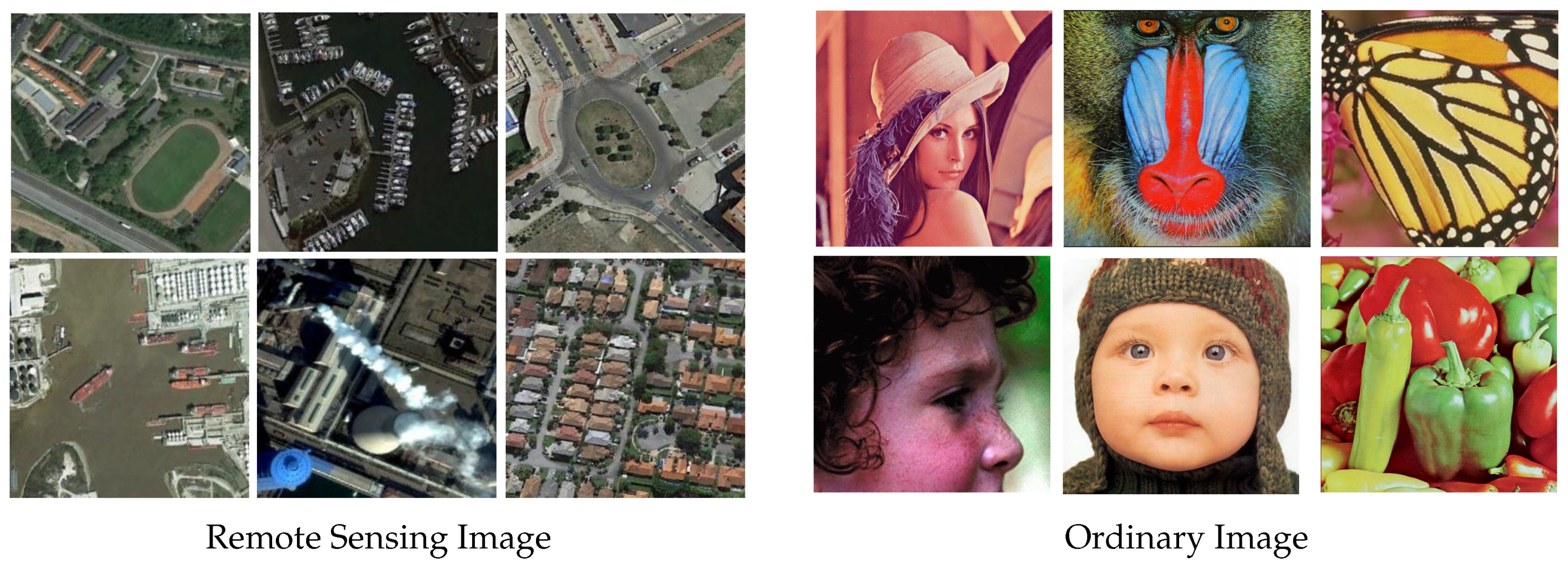
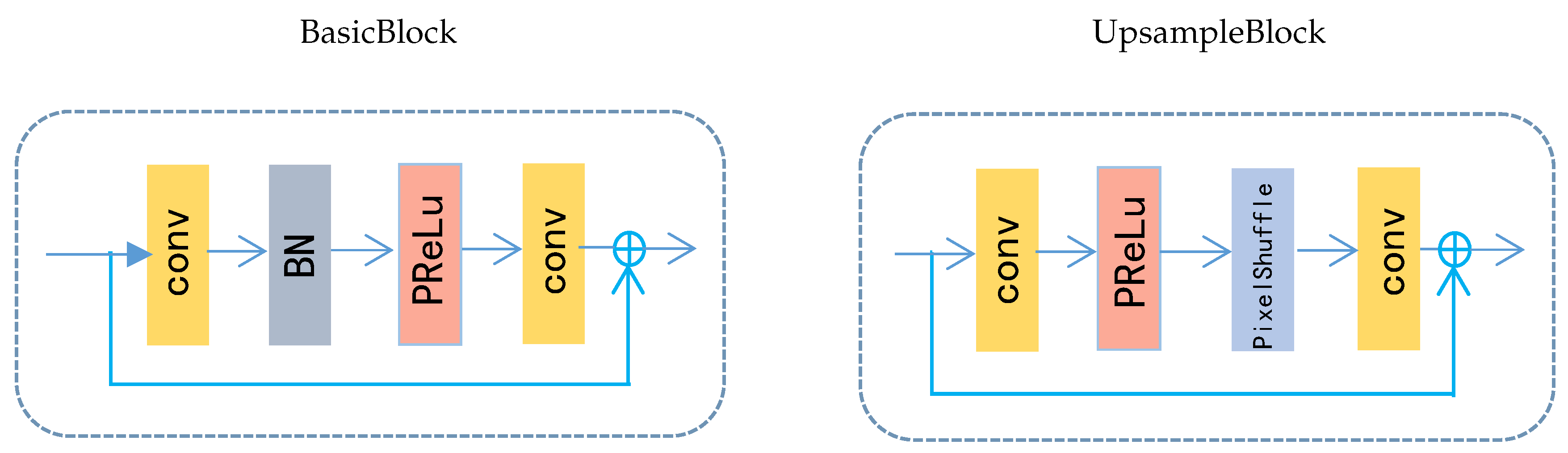
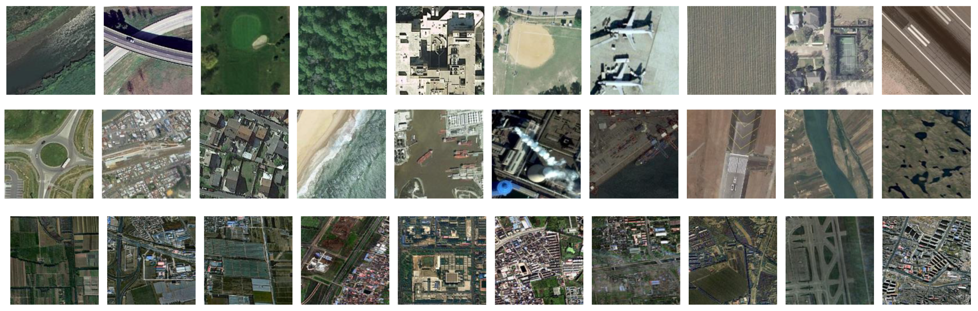
- We choose three representative optical remote sensing datasets with different spatial resolutions to train and test the model. Experiments show that our method outperforms the state-of-the-art algorithms in both super-resolution and denoising tasks. Besides, we apply BN and PReLU for faster convergence and relatively high performance.
2. Related Works
2.1. Traditional Algorithms
2.2. Deep Learning Methods
2.2.1. Image Denoising
2.2.2. Single Image Super Resolution
3. Proposed Deep Connected Neural Network
3.1. Network Architecture
3.2. Downsample Unit and Upsample Unit
3.3. Memory Connection
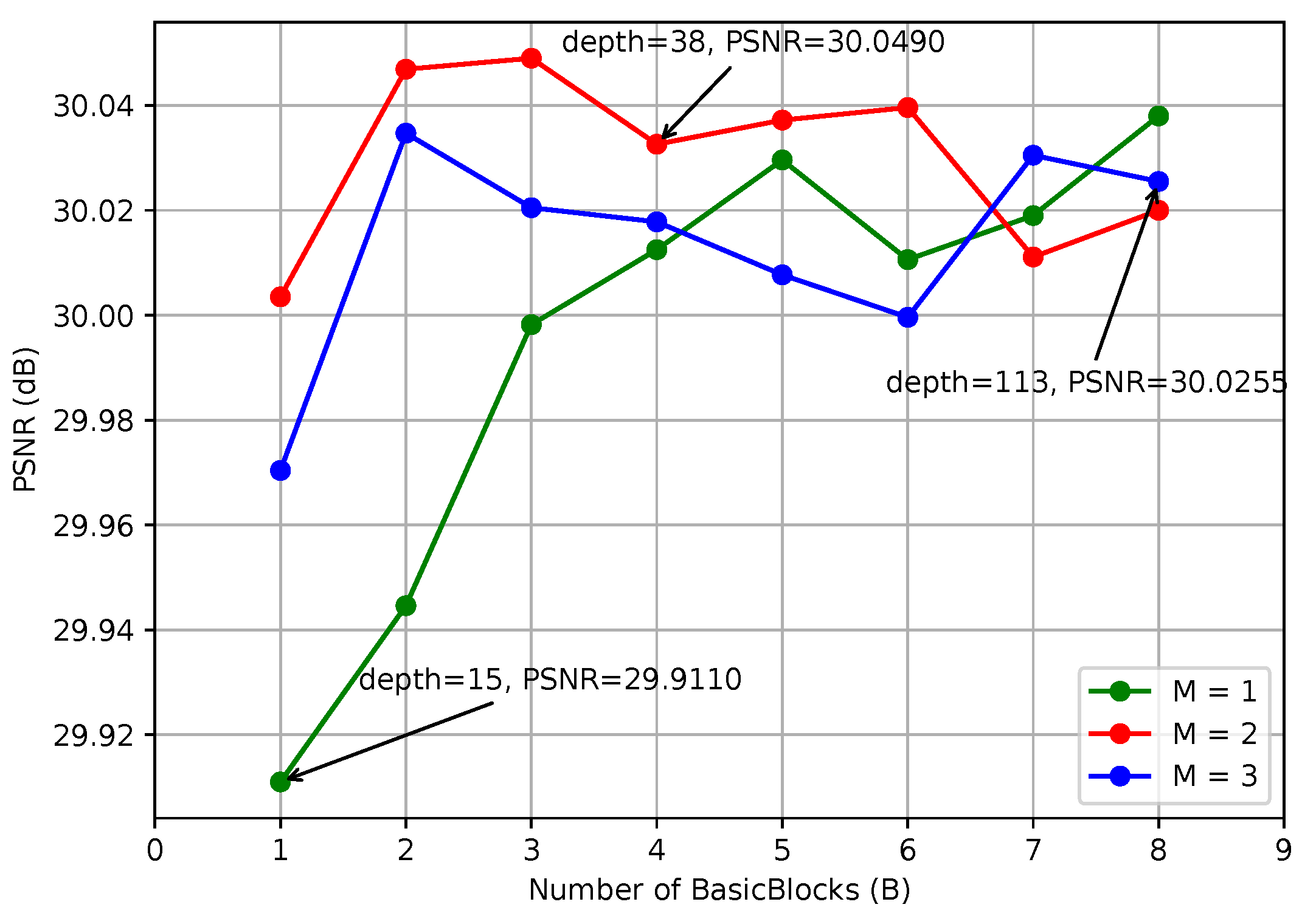
3.4. Network Depth
3.5. Training strategies
4. Experiment
4.1. Dataset Sets and Environmental Configuration
4.2. Network Depth and Width
4.3. Evaluation on Downsample Unit and Upsample Unit
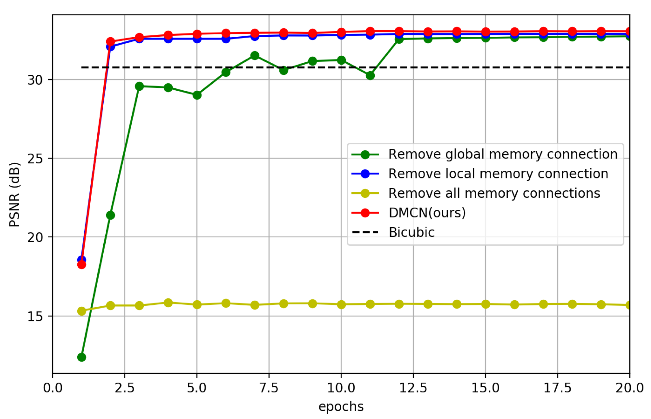
4.4. The Effect of Memory Connection
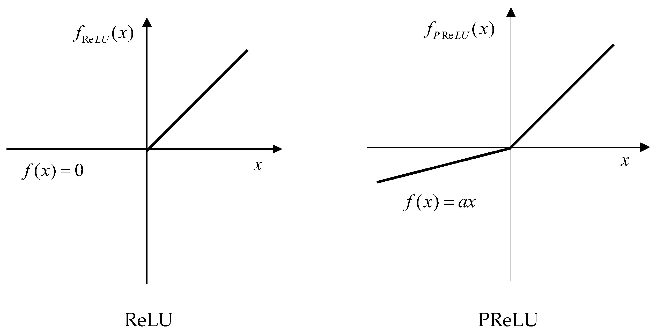
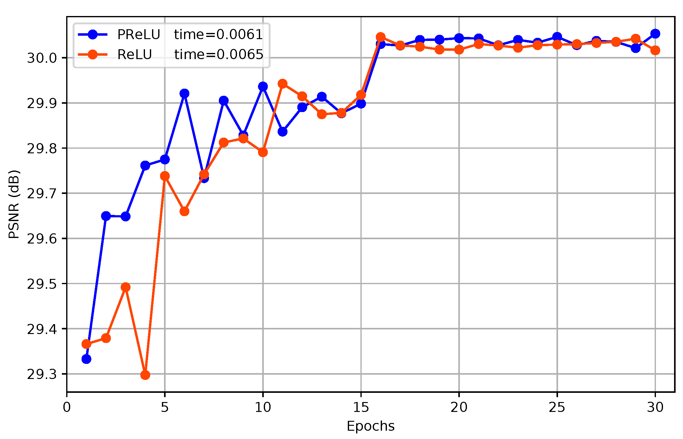
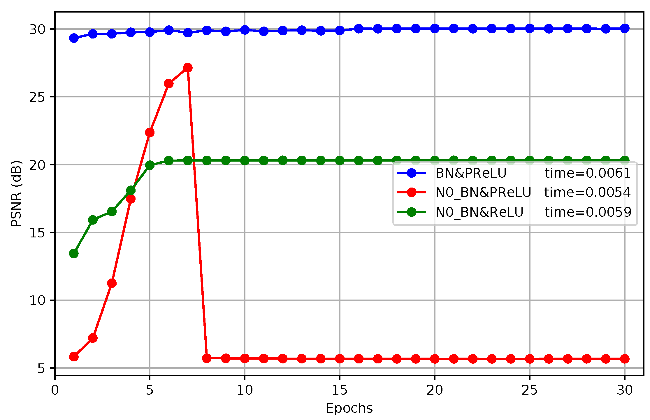
4.5. Batch Normalization and PReLU
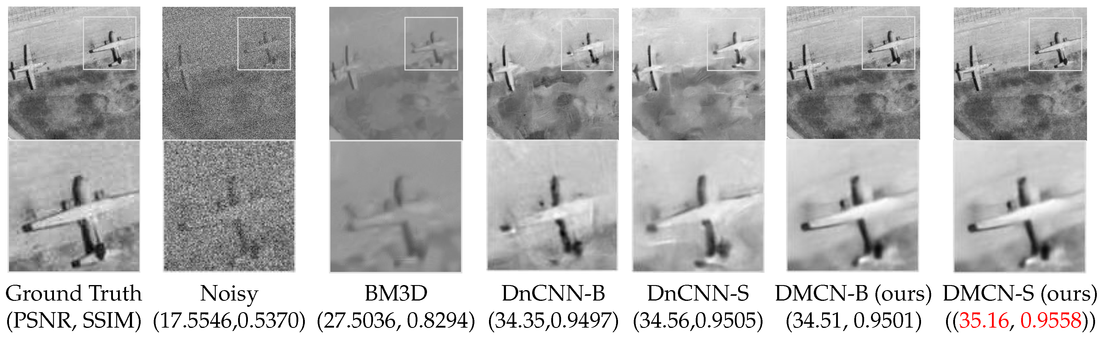
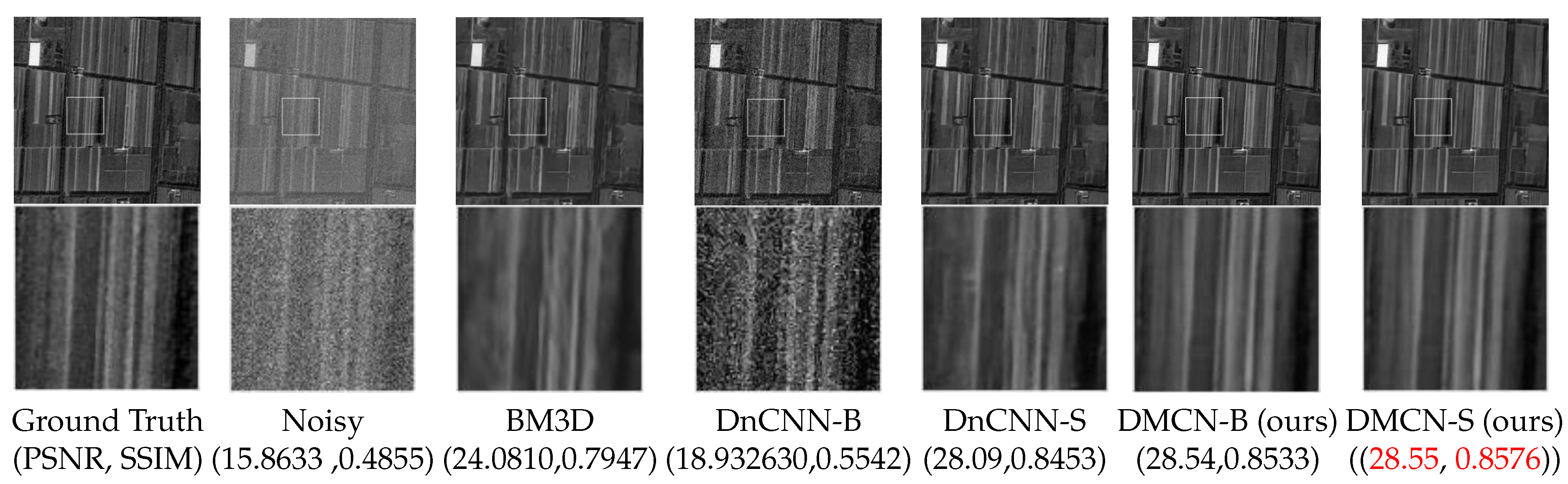
4.6. Gaussian Denoising
4.6.1. Training Details
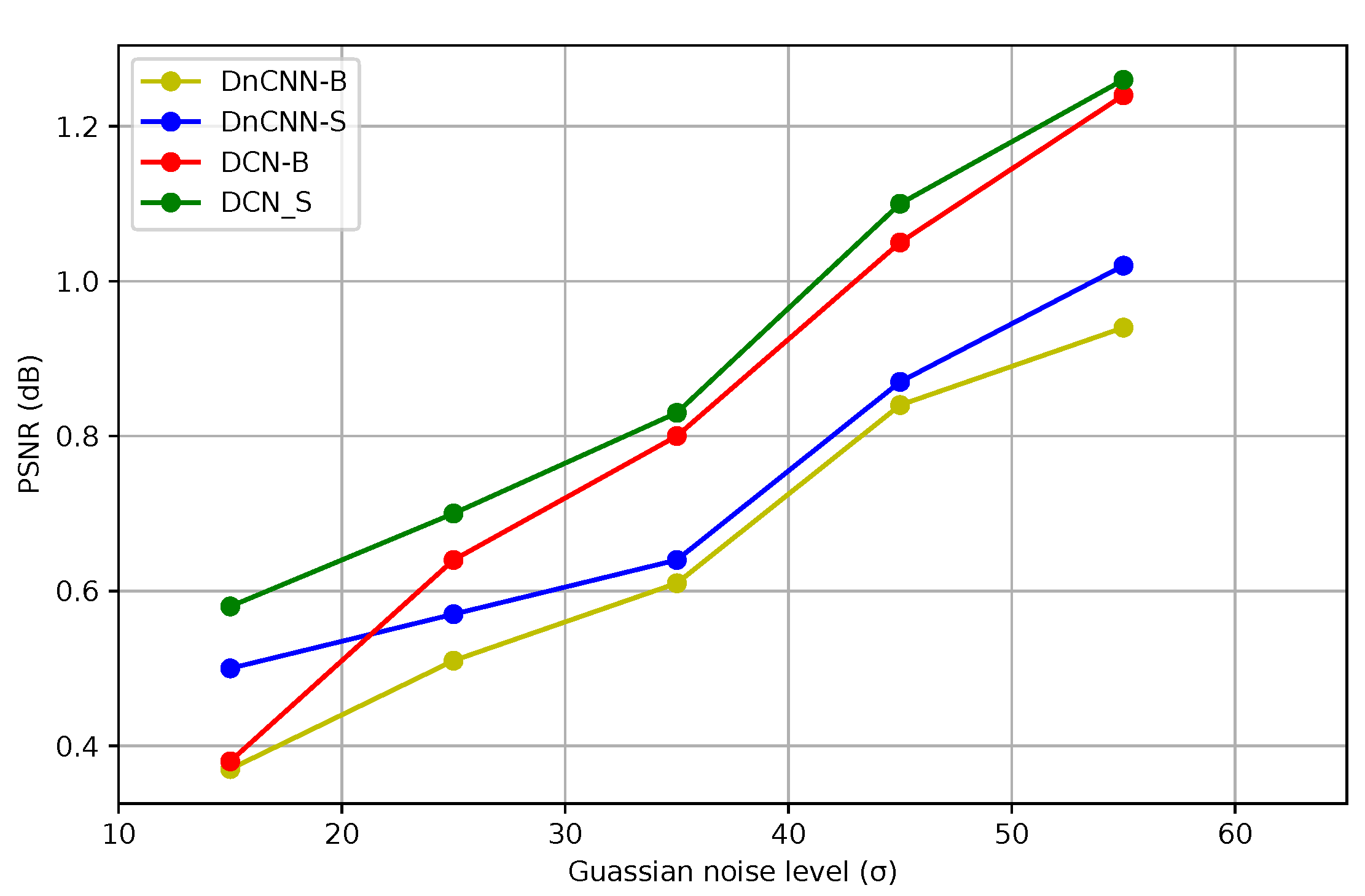
4.6.2. Quantitative Results
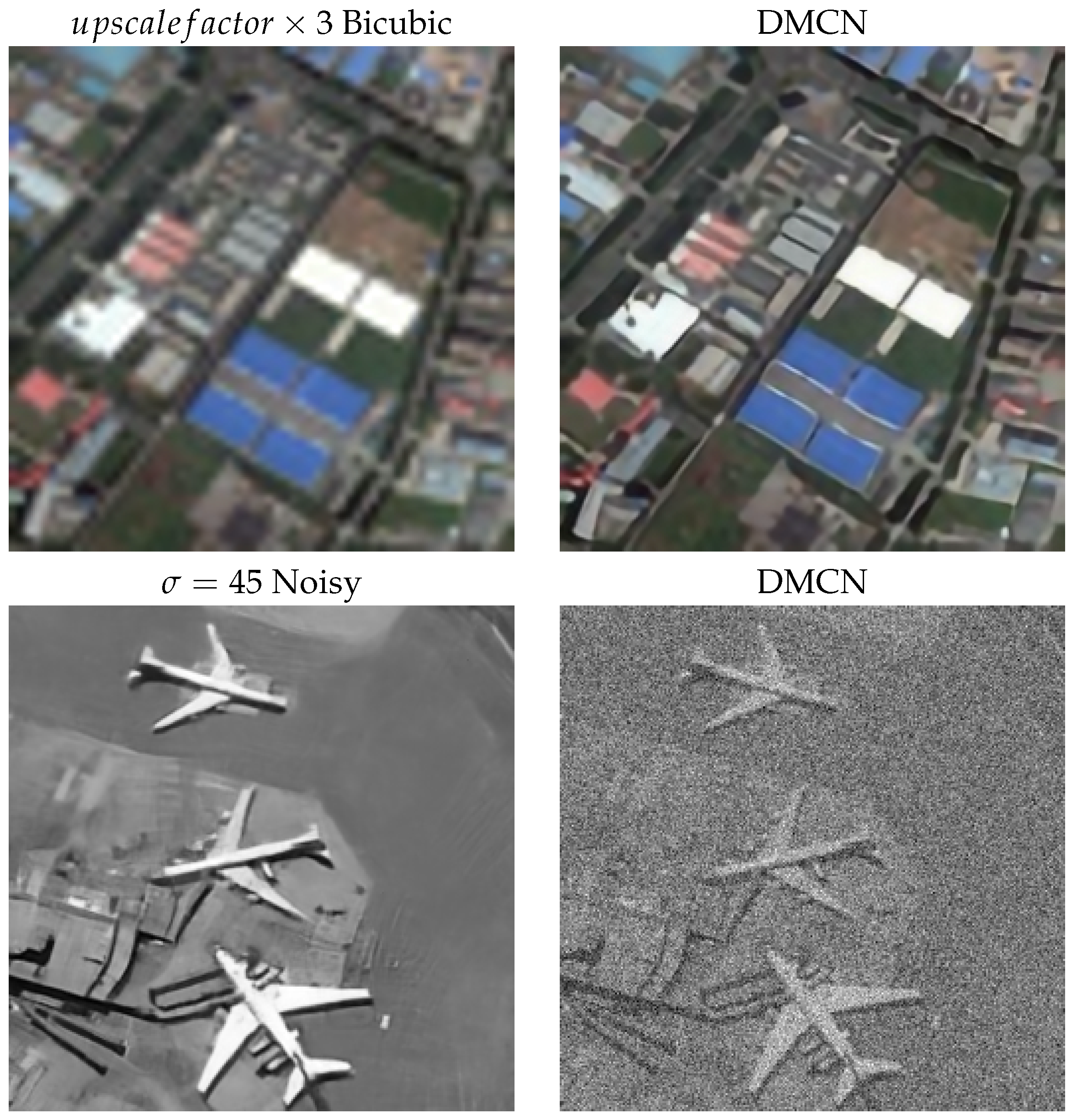
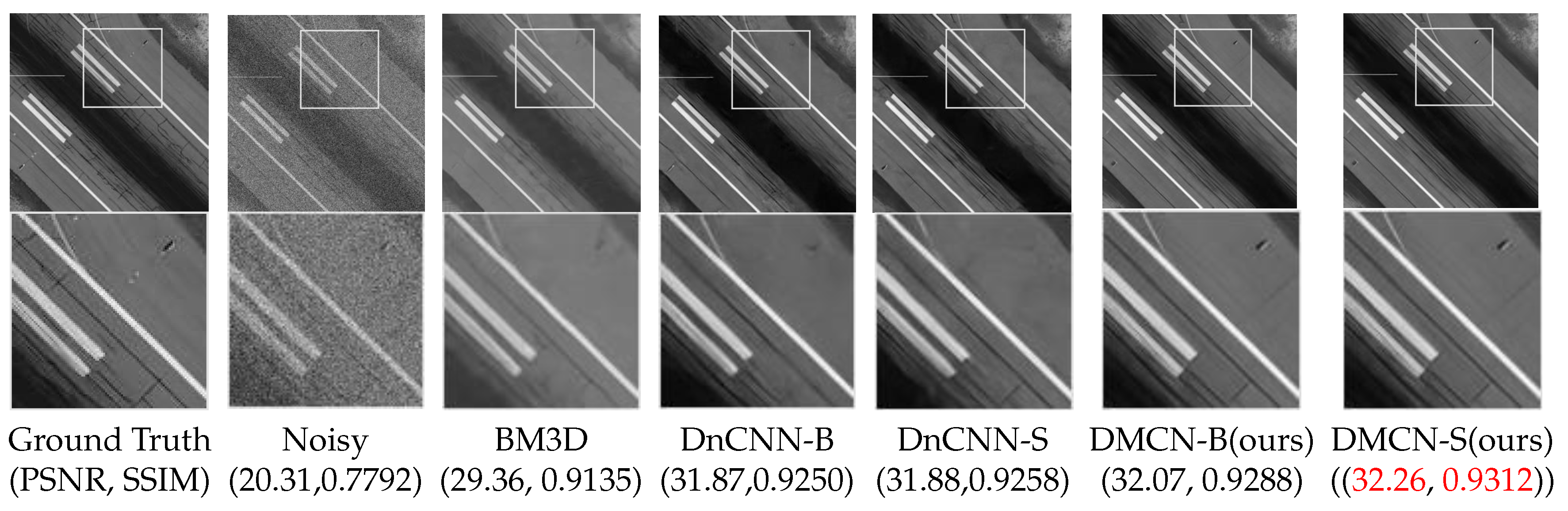
4.6.3. Restored Image Quality
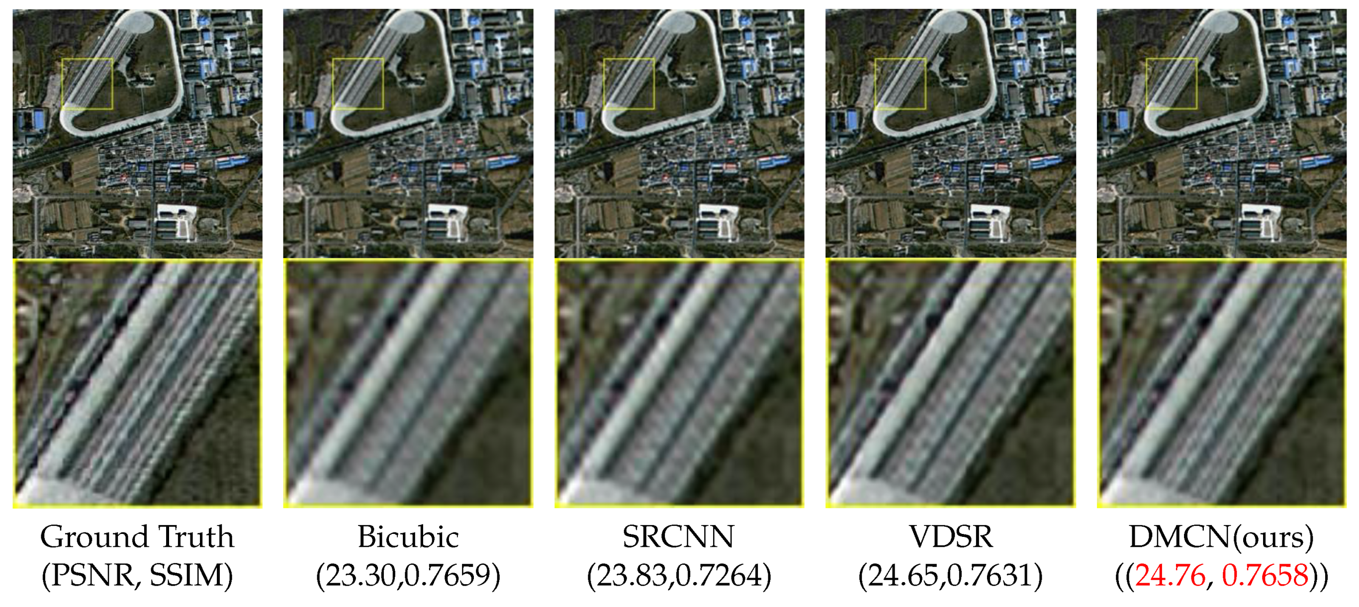
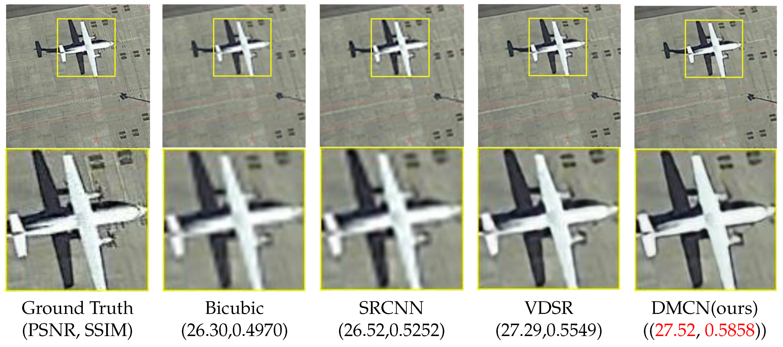
4.7. Single Image Super-Resolution
4.7.1. Training Details
4.7.2. Quantitative Results
4.7.3. Restored Image Quality
5. Conclusions
Author Contributions
Funding
Acknowledgments
Conflicts of Interest
References
- Haut, J.M.; Fernandez-Beltran, R.; Paoletti, M.E.; Plaza, J.; Plaza, A.; Pla, F. A New Deep Generative Network for Unsupervised Remote Sensing Single-Image Super-Resolution. IEEE Trans. Geosci. Remote Sens. 2018. [Google Scholar] [CrossRef]
- Huang, Z.; Zhang, Y.; Li, Q.; Zhang, T.; Sang, N.; Hong, H. Progressive Dual-Domain Filter for Enhancing and Denoising Optical Remote-Sensing Images. IEEE Geosci. Remote Sens. Lett. 2018, 15, 759–763. [Google Scholar] [CrossRef]
- Chang, H.; Yeung, D.Y.; Xiong, Y. Super-resolution through neighbor embedding. In Proceedings of the 2004 IEEE Computer Society Conference on Computer Vision and Pattern Recognition, Washington, DC, USA, 27 June–2 July 2004; Volume 1, p. I. [Google Scholar]
- Freeman, W.T.; Jones, T.R.; Pasztor, E.C. Example-based super-resolution. IEEE Comput. Gr. Appl. 2002, 22, 56–65. [Google Scholar] [CrossRef] [Green Version]
- Dabov, K.; Foi, A.; Katkovnik, V.; Egiazarian, K. Image denoising by sparse 3-D transform-domain collaborative filtering. IEEE Trans. Image Process. 2007, 16, 2080–2095. [Google Scholar] [CrossRef] [PubMed]
- Elad, M.; Aharon, M. Image denoising via sparse and redundant representations over learned dictionaries. IEEE Trans. Image Process. 2006, 15, 3736–3745. [Google Scholar] [CrossRef] [PubMed]
- Dong, W.; Zhang, L.; Shi, G.; Wu, X. Image deblurring and super-resolution by adaptive sparse domain selection and adaptive regularization. IEEE Trans. Image Process. 2011, 20, 1838–1857. [Google Scholar] [CrossRef] [PubMed]
- Yair, N.; Michaeli, T. Multi-Scale Weighted Nuclear Norm Image Restoration. In Proceedings of the IEEE Conference on Computer Vision and Pattern Recognition, Salt Lake City, UT, USA, 18–21 June 2018; pp. 3165–3174. [Google Scholar]
- Gu, S.; Zhang, L.; Zuo, W.; Feng, X. Weighted nuclear norm minimization with application to image denoising. In Proceedings of the IEEE Conference on Computer Vision and Pattern Recognition, Columbus, OH, USA, 23–28 June 2014; pp. 2862–2869. [Google Scholar]
- Dong, C.; Loy, C.C.; He, K.; Tang, X. Learning a deep convolutional network for image super-resolution. In Proceedings of the European Conference on Computer Vision, Zurich, Switzerland, 6–12 September 2014; pp. 184–199. [Google Scholar]
- Zhang, K.; Zuo, W.; Chen, Y.; Meng, D.; Zhang, L. Beyond a gaussian denoiser: Residual learning of deep cnn for image denoising. IEEE Trans. Image Process. 2017, 26, 3142–3155. [Google Scholar] [CrossRef] [PubMed]
- Glorot, X.; Bordes, A.; Bengio, Y. Deep sparse rectifier neural networks. In Proceedings of the Fourteenth International Conference on Artificial Intelligence and Statistics, Ft. Lauderdale, FL, USA, 11–13 April 2011; pp. 315–323. [Google Scholar]
- Ioffe, S.; Szegedy, C. Batch normalization: Accelerating deep network training by reducing internal covariate shift. arXiv, 2015; arXiv:1502.03167. [Google Scholar]
- Haris, M.; Shakhnarovich, G.; Ukita, N. Deep backprojection networks for super-resolution. In Proceedings of the Conference on Computer Vision and Pattern Recognition, Beijing, China, 20 August 2018. [Google Scholar]
- Zhang, Y.; Tian, Y.; Kong, Y.; Zhong, B.; Fu, Y. Residual dense network for image super-resolution. In Proceedings of the IEEE Conference on Computer Vision and Pattern Recognition, Salt Lake City, UT, USA, 18–22 June 2018. [Google Scholar]
- Lim, B.; Son, S.; Kim, H.; Nah, S.; Lee, K.M. Enhanced deep residual networks for single image super-resolution. In Proceedings of the IEEE Conference on Computer Vision and Pattern Recognition (CVPR) Workshops, Honolulu, HI, USA, 21–26 July 2017; Volume 1, p. 4. [Google Scholar]
- Lefkimmiatis, S. Universal Denoising Networks: A Novel CNN Architecture for Image Denoising. In Proceedings of the IEEE Conference on Computer Vision and Pattern Recognition, Salt Lake City, UT, USA, 18–22 June 2018; pp. 3204–3213. [Google Scholar]
- Chen, J.; Chen, J.; Chao, H.; Yang, M. Image Blind Denoising With Generative Adversarial Network Based Noise Modeling. In Proceedings of the IEEE Conference on Computer Vision and Pattern Recognition, Salt Lake City, UT, USA, 18–22 June 2018; pp. 3155–3164. [Google Scholar]
- Cheng, G.; Han, J.; Lu, X. Remote sensing image scene classification: Benchmark and state of the art. Proc. IEEE 2017, 105, 1865–1883. [Google Scholar] [CrossRef]
- He, K.; Zhang, X.; Ren, S.; Sun, J. Deep residual learning for image recognition. In Proceedings of the IEEE Conference on Computer Vision and Pattern Recognition, Las Vegas, NV, USA, 27–30 June 2016; pp. 770–778. [Google Scholar]
- He, K.; Zhang, X.; Ren, S.; Sun, J. Delving deep into rectifiers: Surpassing human-level performance on imagenet classification. In Proceedings of the IEEE International Conference on Computer Vision, Santiago, Chile, 13–16 December 2015; pp. 1026–1034. [Google Scholar]
- Kingma, D.P.; Ba, J. Adam: A method for stochastic optimization. arXiv, 2014; arXiv:1412.6980. [Google Scholar]
- Xu, S.; Zhou, Y.; Xiang, H.; Li, S. Remote Sensing Image Denoising Using Patch Grouping-Based Nonlocal Means Algorithm. IEEE Geosci. Remote Sens. Lett. 2017, 14, 2275–2279. [Google Scholar] [CrossRef]
- Kwan, C.; Zhou, J. Method for Image Denoising. Patent 9,159,121, 13 October 2015. [Google Scholar]
- Chen, Y.; Guo, Y.; Wang, Y.; Wang, D.; Peng, C.; He, G. Denoising of hyperspectral images using nonconvex low rank matrix approximation. IEEE Trans. Geosci. Remote Sens. 2017, 55, 5366–5380. [Google Scholar] [CrossRef]
- Fan, Y.R.; Huang, T.Z.; Zhao, X.L.; Deng, L.J.; Fan, S. Multispectral Image Denoising via Nonlocal Multitask Sparse Learning. Remote Sens. 2018, 10, 116. [Google Scholar] [CrossRef]
- Loncan, L.; Almeida, L.B.; Bioucas-Dias, J.M.; Briottet, X.; Chanussot, J.; Dobigeon, N.; Fabre, S.; Liao, W.; Licciardi, G.A.; Simoes, M.; et al. Hyperspectral pansharpening: A review. arXiv, 2015; arXiv:1504.04531. [Google Scholar] [CrossRef]
- Vivone, G.; Alparone, L.; Chanussot, J.; Dalla Mura, M.; Garzelli, A.; Licciardi, G.A.; Restaino, R.; Wald, L. A critical comparison among pansharpening algorithms. IEEE Trans. Geosci. Remote Sens. 2015, 53, 2565–2586. [Google Scholar] [CrossRef]
- Kwan, C.; Choi, J.; Chan, S.; Zhou, J.; Budavari, B. A super-resolution and fusion approach to enhancing hyperspectral images. Remote Sens. 2018, 10, 1416. [Google Scholar] [CrossRef]
- Vincent, P.; Larochelle, H.; Bengio, Y.; Manzagol, P.A. Extracting and composing robust features with denoising autoencoders. In Proceedings of the 25th International Conference on Machine Learning, Helsinki, Finland, 5–9 July 2008; pp. 1096–1103. [Google Scholar]
- Jain, V.; Seung, S. Natural image denoising with convolutional networks. In Proceedings of the 21st International Conference on Neural Information Processing Systems, Vancouver, BC, Canada, 8–11 December 2008; pp. 769–776. [Google Scholar]
- Chen, Y.; Pock, T. Trainable nonlinear reaction diffusion: A flexible framework for fast and effective image restoration. IEEE Trans. Pattern Anal. Mach. Intell. 2017, 39, 1256–1272. [Google Scholar] [CrossRef] [PubMed]
- Mildenhall, B.; Barron, J.T.; Chen, J.; Sharlet, D.; Ng, R.; Carroll, R. Burst Denoising with Kernel Prediction Networks. In Proceedings of the IEEE Conference on Computer Vision and Pattern Recognition, Salt Lake City, UT, USA, 18–22 June 2018; pp. 2502–2510. [Google Scholar]
- Lehtinen, J.; Munkberg, J.; Hasselgren, J.; Laine, S.; Karras, T.; Aittala, M.; Aila, T. Noise2Noise: Learning Image Restoration without Clean Data. arXiv, 2018; arXiv:1803.04189. [Google Scholar]
- Putzky, P.; Welling, M. Recurrent inference machines for solving inverse problems. arXiv, 2017; arXiv:1706.04008. [Google Scholar]
- Dong, C.; Loy, C.C.; Tang, X. Accelerating the super-resolution convolutional neural network. In Proceedings of the European Conference on Computer Vision, Amsterdam, The Netherlands, 8–16 October 2016; pp. 391–407. [Google Scholar]
- Kim, J.; Kwon Lee, J.; Mu Lee, K. Accurate image super-resolution using very deep convolutional networks. In Proceedings of the IEEE Conference on Computer Vision and Pattern Recognition, Las Vegas, NV, USA, 26 June–1 July 2016; pp. 1646–1654. [Google Scholar]
- Yuan, Y.; Zheng, X.; Lu, X. Hyperspectral image superresolution by transfer learning. IEEE J. Sel. Top. Appl. Earth Obs. Remote Sens. 2017, 10, 1963–1974. [Google Scholar] [CrossRef]
- Qu, Y.; Qi, H.; Kwan, C. Unsupervised Sparse Dirichlet-Net for Hyperspectral Image Super-Resolution. In Proceedings of the IEEE Conference on Computer Vision and Pattern Recognition, Salt Lake City, UT, USA, 18–22 June 2018; pp. 2511–2520. [Google Scholar]
- Shocher, A.; Cohen, N.; Irani, M. Zero-Shot super-resolution using deep internal learning. In Proceedings of the Conference on Computer Vision and Pattern Recognition, Beijing, China, 20 August 2018. [Google Scholar]
- Ledig, C.; Theis, L.; Huszár, F.; Caballero, J.; Cunningham, A.; Acosta, A.; Aitken, A.P.; Tejani, A.; Totz, J.; Wang, Z.; et al. Photo-Realistic Single Image Super-Resolution Using a Generative Adversarial Network. In Proceedings of the CVPR, Honolulu, HI, USA, 22–25 July 2017; Volume 2, p. 4. [Google Scholar]
- Sajjadi, M.S.; Vemulapalli, R.; Brown, M. Frame-Recurrent Video Super-Resolution. In Proceedings of the IEEE Conference on Computer Vision and Pattern Recognition, Salt Lake City, UT, USA, 18–22 June 2018; pp. 6626–6634. [Google Scholar]
- Shi, W.; Caballero, J.; Huszár, F.; Totz, J.; Aitken, A.P.; Bishop, R.; Rueckert, D.; Wang, Z. Real-time single image and video super-resolution using an efficient sub-pixel convolutional neural network. In Proceedings of the IEEE Conference on Computer Vision and Pattern Recognition, Las Vegas, NV, USA, 27–30 June 2016; pp. 1874–1883. [Google Scholar]
- Ronneberger, O.; Fischer, P.; Brox, T. U-net: Convolutional networks for biomedical image segmentation. In Proceedings of the International Conference on Medical Image Computing And Computer-Assisted Intervention, Munich, Germany, 5–9 October 2015; pp. 234–241. [Google Scholar]
- Newell, A.; Yang, K.; Deng, J. Stacked hourglass networks for human pose estimation. In Proceedings of the European Conference on Computer Vision, Amsterdam, The Netherlands, 8–16 October 2016; pp. 483–499. [Google Scholar]
- Yang, Y.; Newsam, S. Bag-of-visual-words and spatial extensions for land-use classification. In Proceedings of the 18th SIGSPATIAL International Conference On Advances in Geographic Information Systems, San Jose, CA, UAS, 3–5 November 2010; pp. 270–279. [Google Scholar]
- Lei, S.; Shi, Z.; Zou, Z. Super-Resolution for Remote Sensing Images via Local-Global Combined Network. IEEE Geosci. Remote Sens. Lett. 2017, 14, 1243–1247. [Google Scholar] [CrossRef]
- Keys, R. Cubic convolution interpolation for digital image processing. IEEE Trans. Acoust. Speech Signal Process. 1981, 29, 1153–1160. [Google Scholar] [CrossRef] [Green Version]
- Timofte, R.; De Smet, V.; Van Gool, L. A+: Adjusted anchored neighborhood regression for fast super-resolution. In Proceedings of the Asian Conference on Computer Vision, Singapore, 1–5 November 2014; pp. 111–126. [Google Scholar]


| Network Width | 32 | 64 | 128 | 256 |
|---|---|---|---|---|
| time(s) | 0.005155 | 0.006224 | 0.007811 | 0.008375 |
| PSNR (dB) | 29.9917 | 30.0554 | 29.9951 | 29.9360 |
| Model | Memory (MB) | Time (Sec) | PSNR |
|---|---|---|---|
| Dis_D_U | 8265 | 0.037 | 34.17 |
| DMCN (ours) | 3849 | 0.012 | 34.19 |
| Dataset | × | Noisy | BM3D [5] | DnCNN-B [11] | DnCNN-S [11] | DMCN-B (Ours) | DMCN-S (Ours) |
|---|---|---|---|---|---|---|---|
| PSNR/SSIM | PSNR/SSIM | PSNR/SSIM | PSNR/SSIM | PSNR/SSIM | PSNR/SSIM | ||
| GF | 15 | 24.75/0.7942 | 30.03/0.9237 | 28.85/0.9082 | 30.57/0.9439 | 30.55/0.9446 | 30.60/0.9445 |
| 25 | 20.49/0.7658 | 27.33/0.8852 | 28.01/0.9053 | 27.99/0.9049 | 28.09/0.9077 | 28.10/0.9069 | |
| 35 | 17.79/0.6221 | 25.58/0.8477 | 23.07/0.7448 | 26.37/0.8689 | 26.52/0.8731 | 26.52/0.8730 | |
| 45 | 15.86/0.4243 | 24.08/0.8221 | 18.79/0.5483 | 25.19/0.8356 | 25.39/0.8409 | 25.36/0.8413 | |
| 55 | 14.38/0.3884 | 22.94/0.7939 | 16.35/0.4301 | 24.29/0.8056 | 24.50/0.8121 | 24.46/0.8123 | |
| UC [46] | 15 | 24.68/0.7928 | 31.80/0.9027 | 32.17/0.9427 | 32.30/0.9450 | 32.18/0.9435 | 32.38/0.9672 |
| 25 | 20.32/0.7530 | 29.37/0.8932 | 29.88/0.9116 | 29.94/0.9132 | 30.01/0.9147 | 30.07/0.9155 | |
| 35 | 17.52/0.7094 | 27.81/0.8659 | 28.42/0.8853 | 28.45/0.8863 | 28.61/0.8896 | 28.64/0.9031 | |
| 45 | 15.50/0.6825 | 26.49/0.8504 | 27.33/0.8614 | 27.36/0.8627 | 27.54/0.8663 | 27.59/0.8649 | |
| 55 | 13.96/0.6177 | 25.47/0.8228 | 26.41/0.8390 | 26.49/0.8399 | 26.71/0.8467 | 26.73/0.8597 | |
| NW [19] | 15 | 24.68/0.8059 | 31.44/0.9339 | 31.80/0.9332 | 31.91/0.9353 | 31.84/0.9351 | 31.98/0.9349 |
| 25 | 20.33/0.7604 | 28.99/0.8827 | 29.49/0.8924 | 29.56/0.8943 | 29.60/0.8962 | 29.64/0.8961 | |
| 35 | 17.55/0.7139 | 27.50/0.8539 | 28.07/0.8575 | 28.13/0.8596 | 28.23/0.8626 | 28.23/0.8633 | |
| 45 | 15.57/0.6855 | 26.28/0.8255 | 27.07/0.8277 | 27.12/0.8305 | 27.22/0.8325 | 27.24/0.8337 | |
| 55 | 14.06/0.6272 | 25.35/0.8004 | 26.27/0.8040 | 26.33/0.8048 | 26.47/0.8085 | 26.49/0.8102 |
| Image Class | Airplane | Basketball-Court | Farmland | Residential | Industrial | Meadow | Stadium |
|---|---|---|---|---|---|---|---|
| DMCN-BM3D | 0.9248 | 1.1370 | 0.5794 | 1.1951 | 0.2366 | 0.2386 | 1.0050 |
| DnCNN-BM3D | 0.7196 | 0.9766 | 0.3044 | 1.0714 | −0.0581 | 0.2031 | 0.8294 |
| Dataset | Scale | Bicubic [48] | A + [49] | NE + NNLS [3] | SRCNN [10] | VDSR [37] | LGCNet [47] | DMCN (Ours) |
|---|---|---|---|---|---|---|---|---|
| PSNR/SSIM | PSNR/SSIM | PSNR/SSIM | PSNR/SSIM | PSNR/SSIM | PSNR/SSIM | PSNR/SSIM | ||
| NWPU-RESISC45 | ×2 | 30.77/0.8172 | 30.86/0.8223 | 30.94/0.8191 | 29.37/0.7598 | 32.77/0.8778 | 32.76/0.8770 | 33.07/0.8842 |
| ×3 | 27.86/0.6405 | 27.92/0.6493 | 27.98/0.6526 | 27.94/0.6545 | 29.28/0.7165 | 29.21/0.7163 | 29.44/0.7251 | |
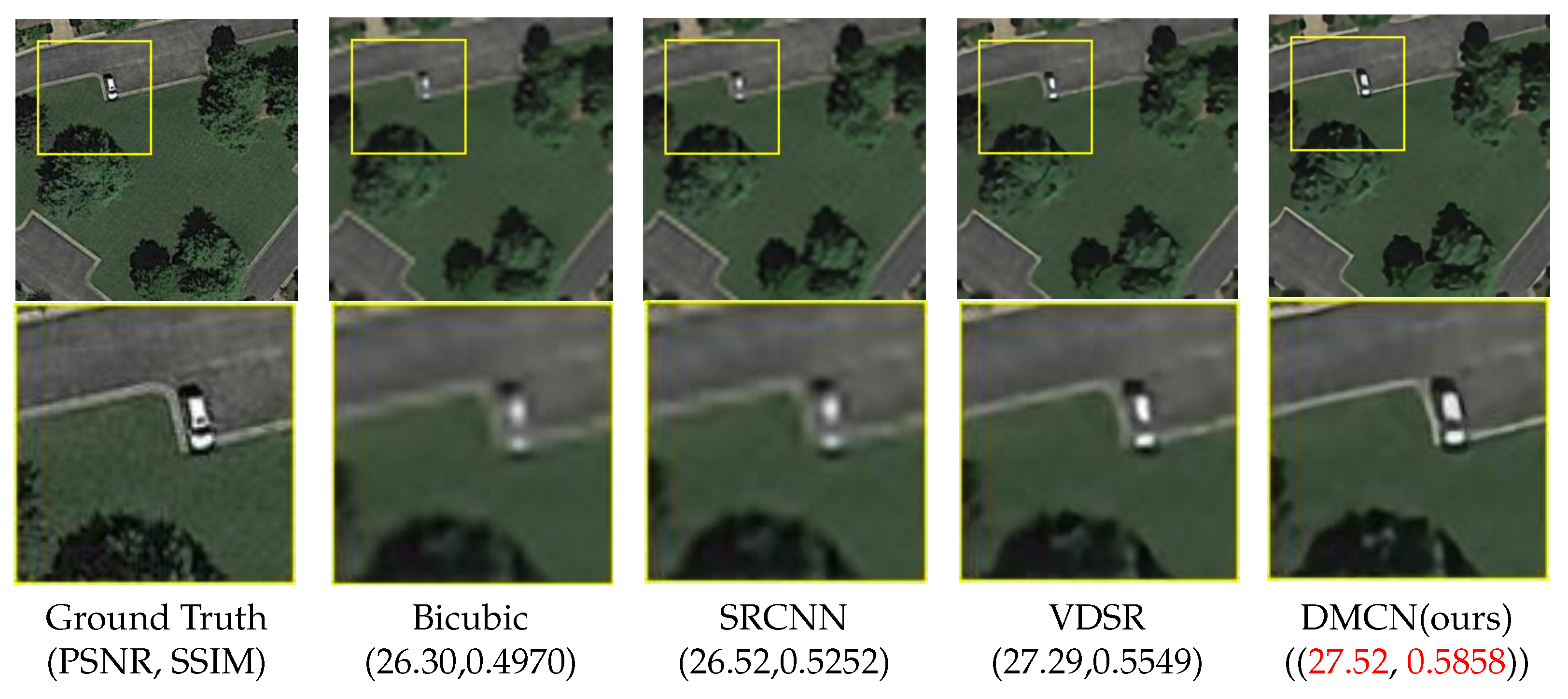
| ×4 | 26.30/0.4970 | 26.41/0.4996 | 26.47/0.5057 | 26.52/0.5252 | 27.30/0.5549 | 27.32/0.5633 | 27.52/0.5858 | |
| UC Merced | ×2 | 31.08/0.8316 | 31.17/ 0.8482 | 31.32/ 0.8530 | 31.06/0.8428 | 33.79/0.8909 | 33.80/0.8817 | 34.19/0.8941 |
| ×3 | 27.59/0.6557 | 27.74/0.6763 | 27.99/0.6898 | 28.24/0.6998 | 29.63/0.7359 | 29.62/0.7350 | 29.86/0.7454 | |
| ×4 | 25.72/0.5800 | 25.91/0.5512 | 25.98/0.5547 | 26.07/0.5439 | 27.31/0.5850 | 27.29/0.5763 | 27.57/0.6150 | |
| GaoFen1 | ×2 | 26.88/0.8585 | 26.93/0.8681 | 27.09/0.8896 | 26.98/0.8727 | 29.23/0.9155 | 29.14/0.9084 | 29.26/0.9250 |
| ×3 | 23.30/0.7263 | 23.56/0.7276 | 23.79/ 0.7261 | 23.83/0.7264 | 24.65/0.7631 | 24.63/0.7602 | 24.76/0.7658 | |
| ×4 | 21.48/0.5039 | 21.60/ 0.5244 | 21.74/0.5470 | 21.78/0.5474 | 22.31/0.5879 | 22.23/0.5834 | 22.38/0.6031 |
© 2018 by the authors. Licensee MDPI, Basel, Switzerland. This article is an open access article distributed under the terms and conditions of the Creative Commons Attribution (CC BY) license (http://creativecommons.org/licenses/by/4.0/).
Share and Cite
Xu, W.; Xu, G.; Wang, Y.; Sun, X.; Lin, D.; Wu, Y. Deep Memory Connected Neural Network for Optical Remote Sensing Image Restoration. Remote Sens. 2018, 10, 1893. https://doi.org/10.3390/rs10121893
Xu W, Xu G, Wang Y, Sun X, Lin D, Wu Y. Deep Memory Connected Neural Network for Optical Remote Sensing Image Restoration. Remote Sensing. 2018; 10(12):1893. https://doi.org/10.3390/rs10121893
Chicago/Turabian StyleXu, Wenjia, Guangluan Xu, Yang Wang, Xian Sun, Daoyu Lin, and Yirong Wu. 2018. "Deep Memory Connected Neural Network for Optical Remote Sensing Image Restoration" Remote Sensing 10, no. 12: 1893. https://doi.org/10.3390/rs10121893
APA StyleXu, W., Xu, G., Wang, Y., Sun, X., Lin, D., & Wu, Y. (2018). Deep Memory Connected Neural Network for Optical Remote Sensing Image Restoration. Remote Sensing, 10(12), 1893. https://doi.org/10.3390/rs10121893