Performance of TRMM TMPA 3B42 V7 in Replicating Daily Rainfall and Regional Rainfall Regimes in the Amazon Basin (1998–2013)

Abstract

Knowledge and studies on precipitation in the Amazon Basin (AB) are determinant for environmental aspects such as hydrology, ecology, as well as for social aspects like agriculture, food security, or health issues. Availability of rainfall data at high spatio-temporal resolution is thus crucial for these purposes. Remote sensing techniques provide extensive spatial coverage compared to ground-based rainfall data but it is imperative to assess the quality of the estimates. Previous studies underline at regional scale in the AB, and for some years, the efficiency of the Tropical Rainfall Measurement Mission (TRMM) 3B42 Version 7 (V7) (hereafter 3B42) daily product data, to provide a good view of the rainfall time variability which is important to understand the impacts of El Nino Southern Oscilation. Then our study aims to enhance the knowledge about the quality of this product on the entire AB and provide a useful understanding about his capacity to reproduce the annual rainfall regimes. For that purpose we compared 3B42 against 205 quality-controlled rain gauge measurements for the period from March 1998 to July 2013, with the aim to know whether 3B42 is reliable for climate studies. Analysis of quantitative (Bias, Relative RMSE) and categorical statistics (POD, FAR) for the whole period show a more accurate spatial distribution of mean daily rainfall estimations in the lowlands than in the Andean regions. In the latter, the location of a rain gauge and its exposure seem to be more relevant to explain mismatches with 3B42 rather than its elevation. In general, a good agreement is observed between rain gauge derived regimes and those from 3B42; however, performance is better in the rainy period. Finally, an original way to validate the estimations is by taking into account the interannual variability of rainfall regimes (i.e., the presence of sub-regimes): four sub-regimes in the northeast AB defined from rain gauges and 3B42 were found to be in good agreement. Furthermore, this work examined whether TRMM 3B42 V7 rainfall estimates for all the grid points in the AB, outgoing longwave radiation (OLR) and water vapor flux patterns are consistent in the northeast of AB.

1. Introduction

The knowledge of climatic patterns and the monitoring of precipitation are essential for the management of water resources, agriculture, transportation, well-being, health monitoring, erosion, and fire [1,2,3,4]. This knowledge, in turn, depends on the availability of rainfall data with adequate spatial and time density. Climatic studies usually rely on long time series (e.g., at least 30 years) to carry out trend analysis. For this reason, and because of their high accuracy, long time series observations from rain gauges are preferred to remote-sensing based estimates. Rain gauges are, however, scarce and unevenly distributed in the Amazon Basin (AB) [2,5,6,7,8], and only provide local information that is hard to extrapolate, especially in the Andes that represent approximately 10% (more than 600,000 km²) of the AB superficies. Indeed, extrapolation could not be representative of the high spatial variability of rainfall in the AB. In contrast, estimated data from remote sensing are attractive as they allow enhancing the spatial information. Nevertheless, satellite products are subject to measurement errors that depend on the geographic context, sensor calibration, and/or algorithm, then they need to be controlled and calibrated, especially with ground data.

The TRMM 3B42 V7 product (afterward 3B42) provide rainfall estimates in the tropics covering nearly three decades (1998–2015). Unlike TRMM 3B42 Real Time product, 3B42 is improved by rain gauges adjustment [9,10]. Despite this adjustment, Delahaye [8] showed many qualitative (hit or miss of rainy events) and quantitative estimation errors in 3B42 version 6 in the Brazilian Legal Amazon. These errors partially arise due to a lower capacity of multi-satellite based algorithms—such as those used by TRMM—to detect warm top stratiform cloud systems [11,12,13] particularly in mountainous regions, where precipitations tend to be underestimated [14,15]. Still, 3B42 generally shows high performance, if not the best, compared to other remote sensing products [8,13,15,16]. The adequacy of rainfall estimates to represent observations is, however, regionally dependent.

The quality of the TRMM products the most recent version of 3B42 (version 7) has been assessed for several tropical regions, some of them focusing on sub-regions of the AB. In the southern tropical Andes [17,18] TRMM 3B42 and TRMM-PR 2A25 (not rainfall adjusted) provide a useful information to characterized the location of the orographic rainfall intensification in the Andean slopes known as rainfall hotspots (more than 4000 mm per year) in the foothills of the Andes. These works also showed that estimations tend to underestimate rainfall by 35% in the hotspots and until 80% in the highlands. In addition, Espinoza et al. [18] and Paccini and al. [19], using TRMM-PR 2A25 and TRMM 3B42 v7 highlight the capacity of 3B42 to capture the intra-seasonal variability of rainfall, in different Andean locations. In lowlands, in the Rio Negro catchment, [20] and in the Amazon Brazilian river basin [21] TRMM 3B42 version 6 tends to underestimates rainfall. Zubieta et al. [22] and Zulkafli et al. [12], showed overestimation of precipitations in the Amazon basin of Ecuador, above all during the dry season. Furthermore, Zubieta et al. [22] concluded that TRMM data are not totally reliable as they do not entirely reproduce the seasonal differences of the Marañón and the Ucayali subcatchments and tend to underestimates rainfall during the dry season. However we do not have yet, an overall assessment of rainfall estimates, in particular taking into account the time accuracy, such the rainfall regime and its changes from a year to the next, for the whole Amazon Basin (AB) and for several decades. The purpose of this study is thus twofold: (i) assess the spatial and time quality of 3B42 in the whole AB, and (ii) assess its ability to reproduce rainfall regimes at several time and spatial scales, by comparing rain gauge data against 3B42 gridded values.

The paper is organized as follows: in Section 2, we present the study area, the data and the methodology. The results of 3B42 performance are presented in three main parts in Section 3: first, quantitative and qualitative statistical tools are applied to daily values for the whole period 1998–2013. Secondly, we address the capacity of 3B42 to reproduce the rainfall regimes of the different regions of the AB and their time variability which makes it possible to define sub-regimes. Finally, we examine the coherence of 3B42 derived rainfall patterns with outgoing longwave radiation (OLR) and try to explain them using water vapor fluxes over South America. Conclusions and final remarks are presented in Section 4.

2. Data and Methodology

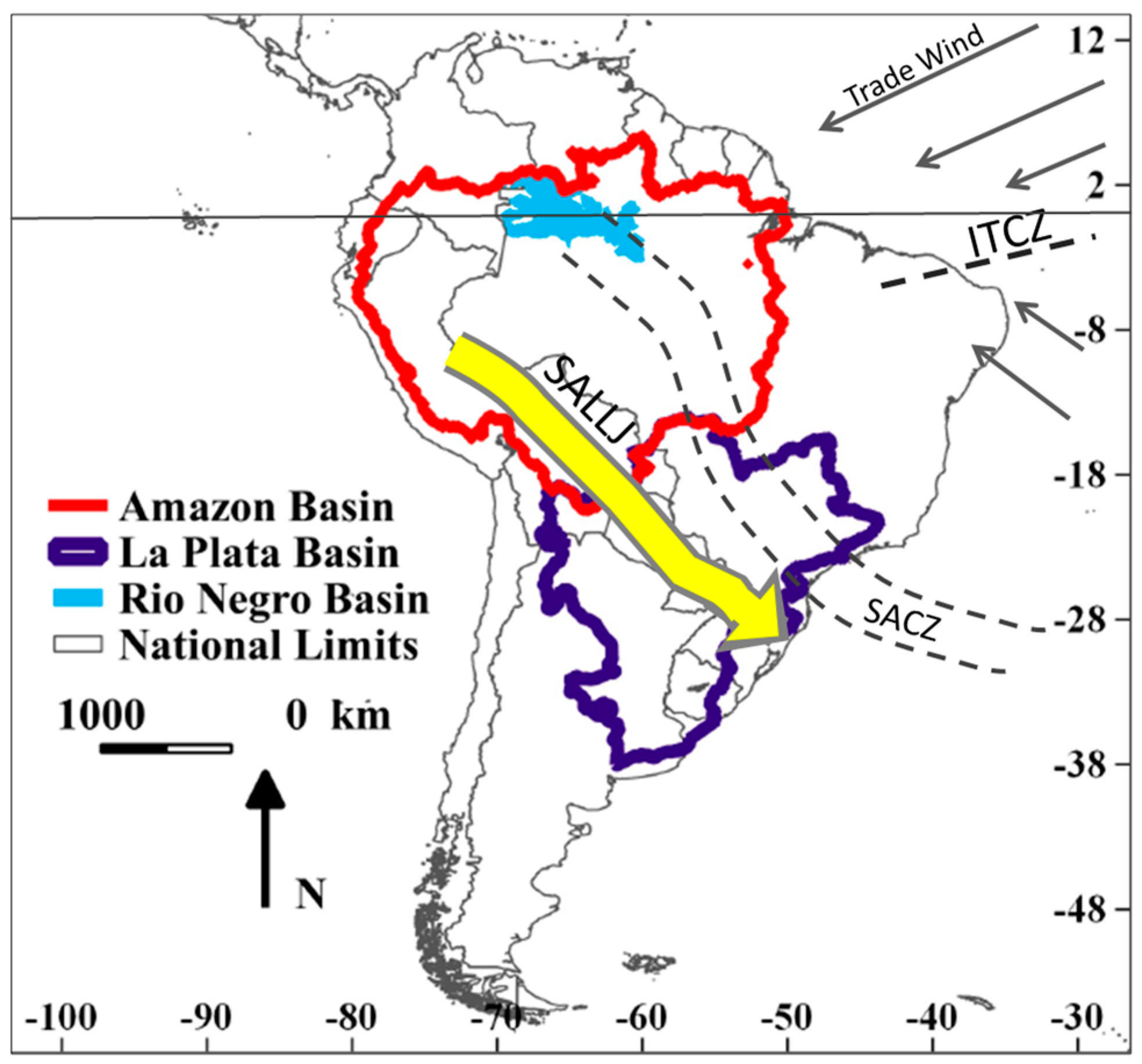
2.1. Study Area

The AB is located in the intertropical zone, between 6° N and 20.5° S and between 48.5° W and 80.5° W (Figure 1 and Figure 2). The AB presents strong topographic contrasts between highlands in the Andean mountains in its western and southwestern parts and lowlands in its central, northern, and eastern parts. The South American Monsoon System (SAMS) [23,24,25,26] is the most important climatic feature affecting the region. During the rainy season, typically spanning from October to March, the South American continent warms up and generates the advection of humidity from the northern tropical Atlantic to the AB and until the La Plata basin by the low level jet (LLJ; Figure 1). This increase in humidity in the La Plata basin helps support the South Atlantic Convergence Zone (SACZ) and its associated heavy rainfall. Conversely, from April to September the SAMS moves into its dry phase in most of the AB. The large latitudinal amplitude and the variety of topographical characteristics give rise to a number of rainfall regimes in the AB poorer [27,28,29], among others]: equatorial in the west and along the Negro Basin (Figure 1); with a dry and a rainy season in the tropical regions of the basin. Over the Atlantic Ocean the convergence of northern and southern trade winds forms the Intertropical Convergence Zone (ITCZ; Figure 1), characterized by strong convection. The equatorial and tropical Atlantic also warm up at the end of the austral summer leading to the southward migration of the ITCZ, and the triggering of the rainy season in the northeast AB.

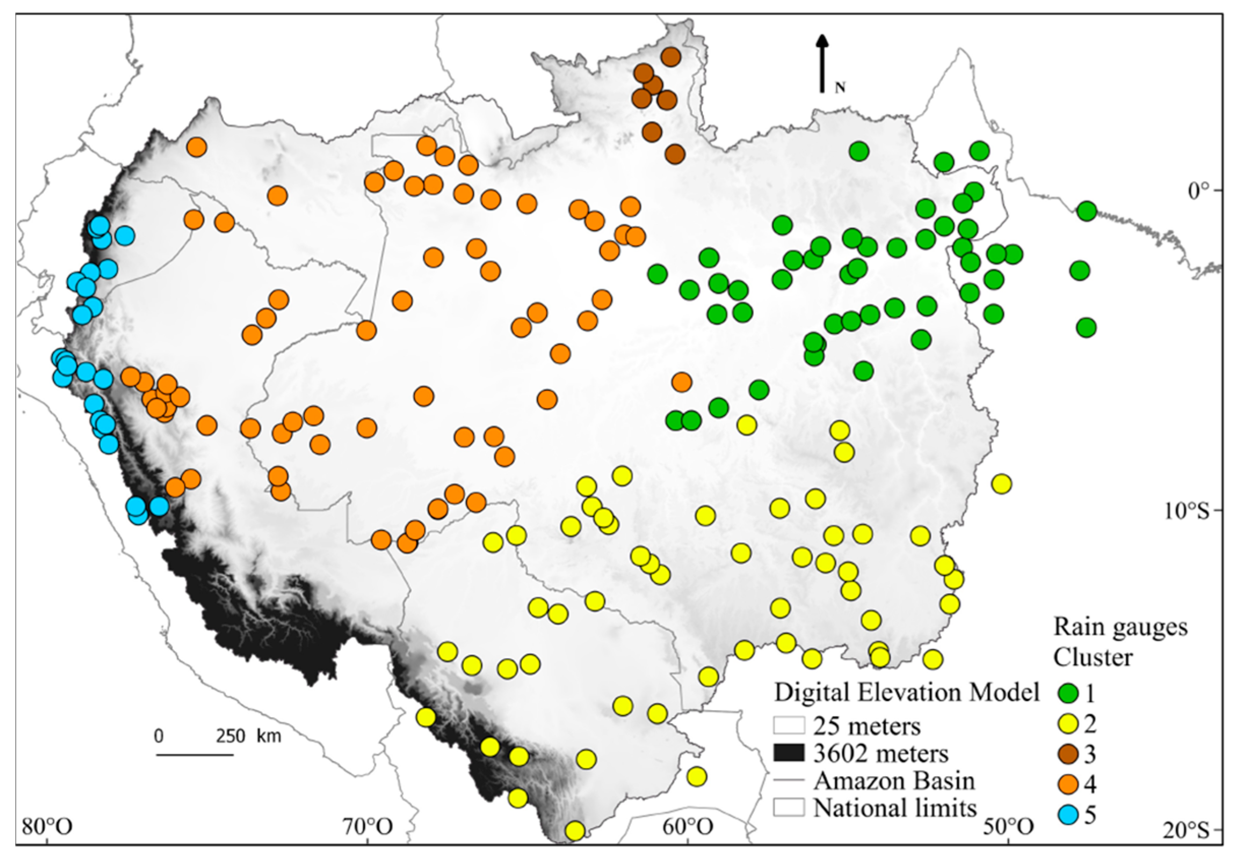
2.2. Observed Precipitations: Rain Gauge Data

The network of observed daily data used as a reference to validate 3B42 estimated data consists of 205 rain gauges (geographically distributed as shown in Figure 2) that have less than 20% missing values and have been quality controlled [30,31]. However, the lack of rain gauges metadata avoid to provide information like the kind device, and then know their accuracy, which could be of great interest when comparing observed and estimated data.

The study covers the period from March 1998 to July 2013. These data were obtained from the National Water Agency (ANA) and the National Meteorological Institute (INMET) in Brazil, the National Meteorological and Hydrological Institute (INAMHI) in Ecuador, the Hydrological Meteorological and Environmental Studies Institute (IDEAM) in Colombia, and the National Hydrological and Meteorological Service (SENAMHI) in Peru and Bolivia. Unfortunately, no such data could be collected in Venezuela.

2.3. Estimated Precipitations: TRMM TMPA 3B42 Version 7 Daily Product

The 3B42 daily product is computed using the TRMM Multisatellite Precipitation Analysis (TMPA) algorithm, developed by the NASA Goddard Space Flight Center [32]. It consists in a gridded precipitation product with a spatial resolution of 0.25° × 0.25° (approximately 25 × 25 km near the equator) and is available between 50° N and 50° S. This product is gauge-adjusted, but the independence between estimated and observed data is assumed because rain gauge network used in 3B42 comes from monthly estimates from the Global Precipitation Climatology Centre product, which only have few gauges in the AB. The TMPA algorithm combines multiple independent precipitation estimates from multiple instruments on board: the Advanced Microwave Scanning Radiometer for Earth Observing Systems (AMSR-E), Special Sensor Microwave Imager (SSMI), Special Sensor Microwave Imager/Sounder (SSMIS), Advanced Microwave Sounding Unit (AMSU), and Microwave Humidity Sounder (MHS), each calibrated to the TRMM Combined Instrument (TCI). Coverage gaps in space and time are completed with merged and microwave-adjusted geo-infrared (IR) data.

2.4. Outgoing Longwave Radiation and Water Vapor Flux

The satellite measures of OLR were obtained from the National Center for Atmospheric Research of the National Ocean and Atmospheric Administration (NCAR/NOAA) [33] and water vapor flux reanalysis [34] is from the National Center for Environmental Prediction (NCEP{XE “NCEP-NCAR” \t “National Center for Environnemental Prediction—National Center for Atmospheric Research”}). The water vapor flux is computed from the specific humidity and the horizontal wind (zonal -u-) from the ground to 300 h Pa [35] as:

$$F_W=\int q V p/g$$

(1)

where q is the humidity, V is the wind vector, p is the pressure, and g is the acceleration due to gravity.

2.5. Intercomparison Methodology

2.5.1. Daily Rainfall Values

Because of the impossibility to extrapolate the scarce rain gauge network, the comparison between observed and estimated data is based on a point-to-pixel approach, using the pixel that contains the rain gauge (hereafter the 3B42 pixel). This approach was already used in the AB in previous studies and gave accurate results [21,36]. Furthermore, Demirtas et al. showed that quantitative precipitation forecast verification with either a grid to grid or grid to point approach give close results.

The quantitative statistics used in this work are the mean daily rainfall, the Bias Equation (1) and the relative root-mean-square error (relative RMSE, Equation (2)) while the categorical statistics are the probability of detection (POD, Equation (3)) and the False Alarm Ratio (FAR, Equation (4)). These statistics are defined as:

$$Bias=100\frac{{{\displaystyle \sum }}_{i=1}^N\left(Pe,i-Po, i\right)}{{{\displaystyle \sum }}_{i=1}^{N}Po, i}$$

(2)

$$Relative RMSE= \sqrt{\frac{{{\displaystyle \sum }}_{i=1}^N\left(Po, i-Pe,i\right)²}{n}}/\overline{Po}$$

(3)

$$POD=\frac{H}{H+M}$$

(4)

$$FAR=\frac{F}{H+F}$$

(5)

where Pe, I is the estimate and Po, I the observation for the i-th day; N is the total number of days, $/\overline{Po}$ is the mean observed precipitation in the whole period, H (hit) is a precipitation event observed by the rain gauge and also detected by 3B42; M (miss) is a precipitation event observed by the rain gauge but not detected by 3B42; F (false alarm) is a precipitation event detected by 3B42 but not observed by the rain gauge. The bias indicates the overestimation or the underestimation by 3B42 in percentage. The relative RMSE gives an average of the error of 3B42, in millimeter (mm). The POD measures the number of rainfall events correctly detected by the estimated product with values ranging between 1 (a perfect score) and 0. The FAR measures the fraction of wrong events detected by 3B42 with values ranging between 1 (the worst score) and 0. The threshold for determining the occurrence of a rain event is set here at 0.1mm in order to avoid the difference in measurement resolution between the two datasets. Indeed, the data from the rain gauges have a resolution of one decimal while 3B42 has several decimals. It is therefore necessary to take it into account in order not to bias the FAR.

In order to assess how well the estimated product reproduces the diversity of rainfall regimes within the AB, the performance of 3B42 is assessed using the standard statistical methods above mentioned at regional scale and for each month of the year. Results of the comparisons are examined, whenever relevant, in the context of the geographical characteristics of the stations (elevation, windward or leeward position).

2.5.2. Rainfall Regimes

In addition to the time-averaged, global 3B42 quality assessment, observed and estimated regional mean annual rainfall and regimes have been computed for five regions, defined using a spectral clustering method [37,38], within the AB (Figure 2). The main principle of spectral clustering is to represent all rain gauges in separate nodes of a connected graph whose vertexes express the similarity between two nodes. The spectral analysis of this graph enables to isolate its main consistent groups. To compute the connection between two nodes into this graph, the basic solution consists in computing a simple Euclidian distance. However, in order to estimate clusters separated in a non-linear way, we exploit the kernel trick. The idea consists in projecting data in another space than the usual one (represented by multi-variate vectors where each component is a value of precipitation) where the separation between clusters is linear. Under some specific properties (see Camps-Valls et Bruzzone [38] for a complete theory of kernels), this projection can simply be done by changing the way one computes the connection between nodes. In practice, this is done using a Gaussian kernel where the connection between two rain gauges ${\mathrm{x}}_1$ and ${\mathrm{x}}_2$ is:

$$\mathrm{K}\left({\mathrm{x}}_1,{\mathrm{x}}_2\right)={\mathrm{e}}^{-\frac{\Vert {\mathrm{x}}_1-{\mathrm{x}}_2\Vert }{{\mathsf{\sigma }}^2}}$$

(6)

where $\mathsf{\sigma }$ is a parameter to fix. It has been proven that this kernel enables to efficiently separate highly non-linear clusters.

The determination of the optimal number of clusters is an open problem for which no sound solution exists at the moment. In this study, we rely on the intra/inter inertia. More precisely, a reliable clustering should reveal both homogeneity inside clusters (all stations of the same group are similar) and heterogeneity between averaged clusters (all clusters represent different groups). Therefore, the ratio between the inertia among (averaged) clusters and the internal inertia (sum on inertia inside all groups) should be maximal. The ratio find here is reached when defining 12 clusters. Afterward, small clusters (less than five rain gauges) are gathered with the nearest cluster (taking into account the spatial and interclass variance). The resulting regionalization in Figure 2 is consistent with former studies, showing for example the separation between tropical and equatorial regions and between highlands and lowlands [27,29,39,40]. Finally, these regions, have similar rainfall regimes, and were named according to their relative position within the AB—northeast, south, north, center, and west—as shown in Figure 2.

Then, sub-regimes for each region, based on spectral clustering approach, were also defined in order to assess the interannual variability of regional rainfall patterns. We obtained, for each region, several groups of years—or, clusters—presenting the same type of rainfall sub-regime. Next, based on these clusters rainfall sub-regimes were computed using 3B42. Notice that different clusters not necessarily include the same number of years

Finally, water vapor fluxes and outgoing longwave radiation (OLR) anomalies were compared to precipitation patterns derived from 3B42 all grid point in order (1) to confirm the precipitation patterns and (2) to give some explanations to the observed anomalies. Indeed, OLR is commonly used as proxy for convection in the Tropical region and water vapor fluxes in the AB play an important role in the precipitation variability, and OLR is commonly used as proxy for convection in the Tropical region.

3. Results and Discussion

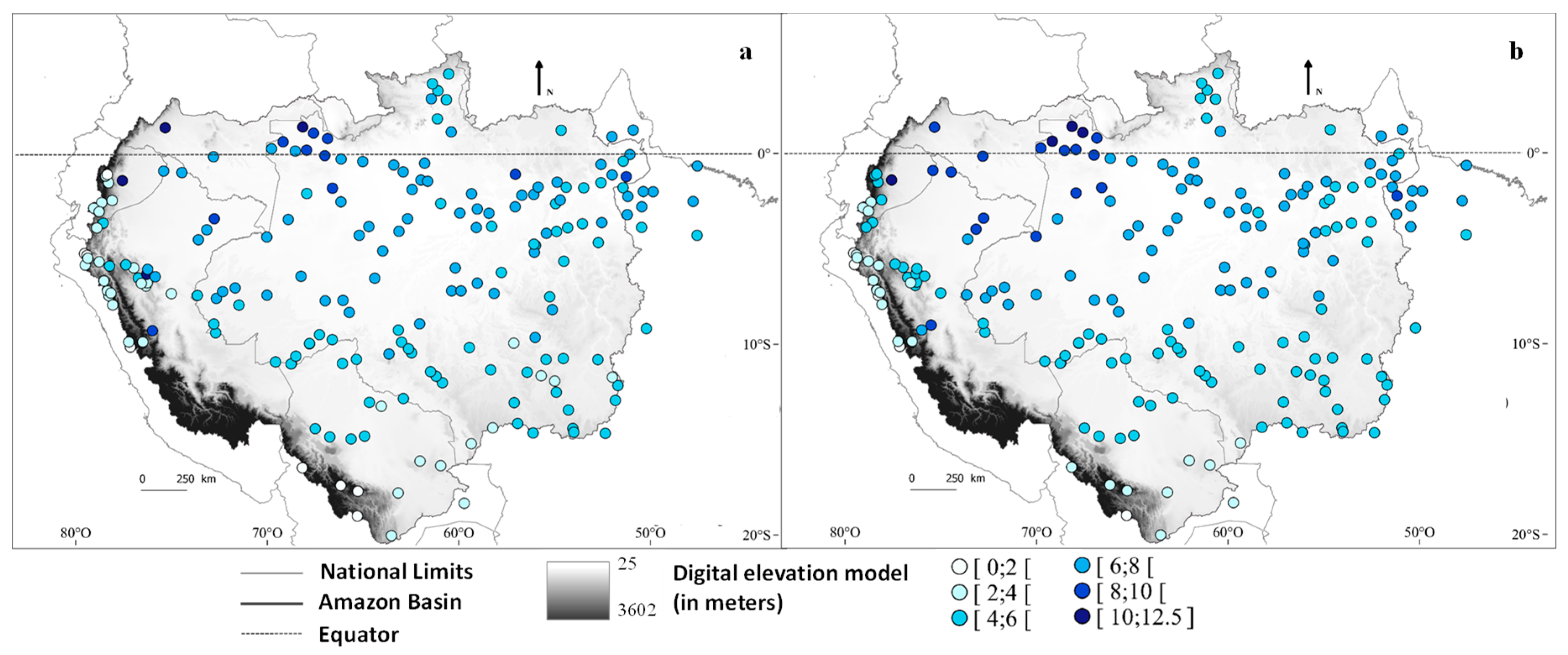
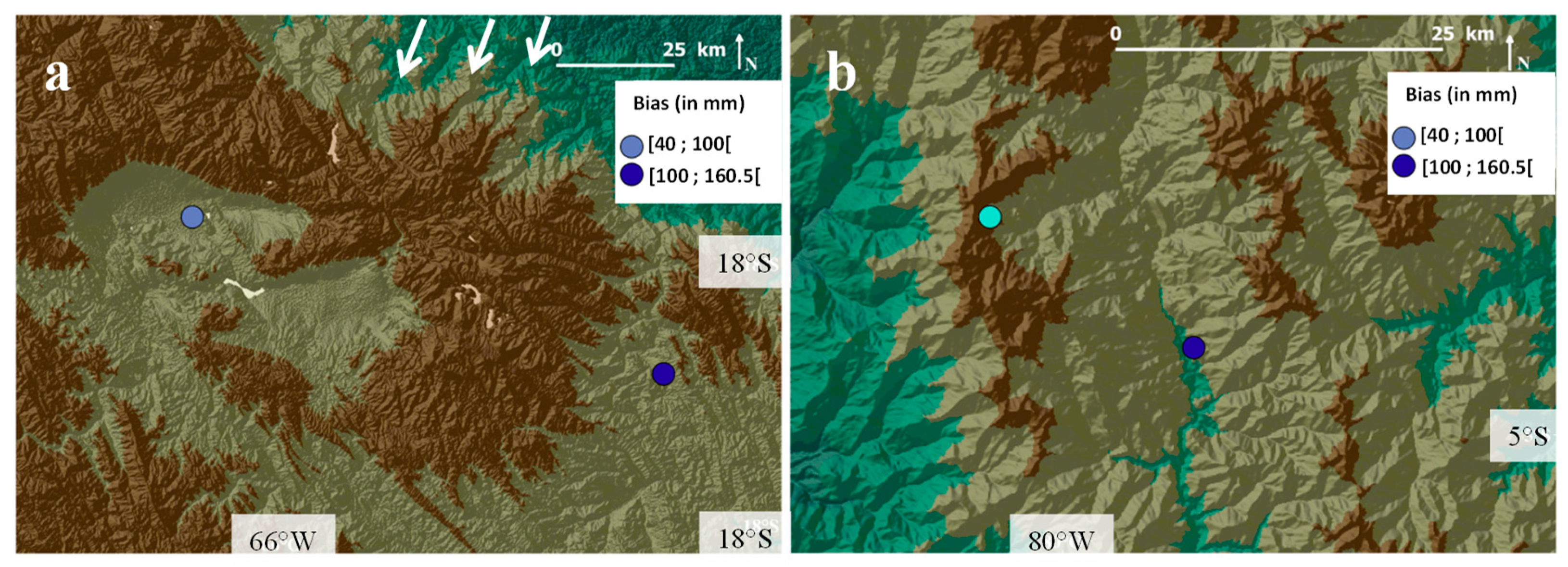
3.1. Comparison between Points and Pixels at Annual and Monthly Time Scales

At large scale, for the whole AB, 3B42 reproduces well the spatial distribution of mean daily rainfall (Figure 3a,b), with the highest rates of rainfall near the equator while rainfall decreases southward and northward at tropical latitudes. The lowest values are in the Andes, as shown previously. However, 3B42 tends to overestimate rainfall in the lowlands. In the mountains the results vary from one region to another. Indeed, differences can be observed between the northern, central and southern parts of the Andes. In the central part of the Andes, the underestimation is stronger than in the northern part, and rainfall is overestimated in the southern part of the Andes.

The other indicators also depict these differences between lowlands and highlands and within the highlands. The most relevant is the bias (Figure 4a) which shows (a) a null or positive bias in most stations (until +161%), meaning that the estimated values are higher than the observations, and (b) extreme values in the Andean mountains [−45.5; 40] and [+100; +161]% and some exceptions in the northeast and south regions [−40; 35] and [+10; 100]%. In the Andes the bias are positive (until +161%) in most stations of Ecuador (northern Andes), which is coherent with Zubieta et al. [22] and Zulkafli et al. [12] and Bolivia (southern Andes), while the bias is generally negative (until −45.5%) in Peru (Central Andes). This contrast between northern and central Andes was also observed by Zulkafli et al. [12] while the heterogeneity of the bias was found by Salio et al. [13] for the Brazilian and Bolivian Amazon. Two main hypotheses can be proposed to explain these bias. The first is the location and the leeward or windward exposition of the rain gauges in each region, this point will be discussed later. However, as it is unlikely that all the stations are located leeward or windward, another possibility is that the type of rain gauge differs between the countries and/or during the time series, and have different calibration. Indeed, some rain gauges, those using tipping bucket, can have less precision due to the time to fill the bucket and then to make it tip and register the amount of precipitation during light rainfall. Furthermore, a high evaporation can also cause a lower accuracy of the rain gauge by avoiding a good tipping of the bucket [41,42], because of a same order of magnitude of the precipitation and evaporation rate. Unfortunately, we do not have such information about the rain gauge stations.

The RMSE (Figure 4b) for most stations was found to be smaller than 3 mm/day, but in some Andean stations and in the southern tropics the RMSE reached values as high as 7 mm/day.

Better results are also observed in the lowlands with the categorical statistics. Indeed, the POD values indicate a good detection (POD > 0.7) of rainy events by the estimated product along a diagonal from northwestern to southeastern Amazon, i.e., along the mean position of the South Atlantic Convergence Zone that produces heavy rainfall in summer (Figure 5a). There is a correct detection of rainy events in the central and southern Andes. The worst values are observed in the northern part of the Andes, in the Bolivian lowlands, and northeast AB.

The false detection of rainy events (FAR) shows on the one hand the Andes and the south of the AB, both of which with the worst results, and on the other, the equatorial and northern locations that show pretty good results (Figure 5b). Globally the results are good with values mainly below 0.58, and there are not clear intra-Andean differences, as observed with other indicators.

Furthermore, as rainfall changes during the year, we computed the Bias, the relative RMSE, the POD and the FAR (Figure 6) at monthly time scale. The results show a contrast between the rainy and the dry seasons, with a higher occurrence of low POD (until 0) and high FAR (until 1), a higher bias (until 300%) and RMSE (until 24 mm) during the driest months. However, since it exists a large range of rainfall regimes in the AB, these time differences could represent only a part of the intra-annual variability, then, a further spatial analysis is needed to better known if that variability is regionally dependent.

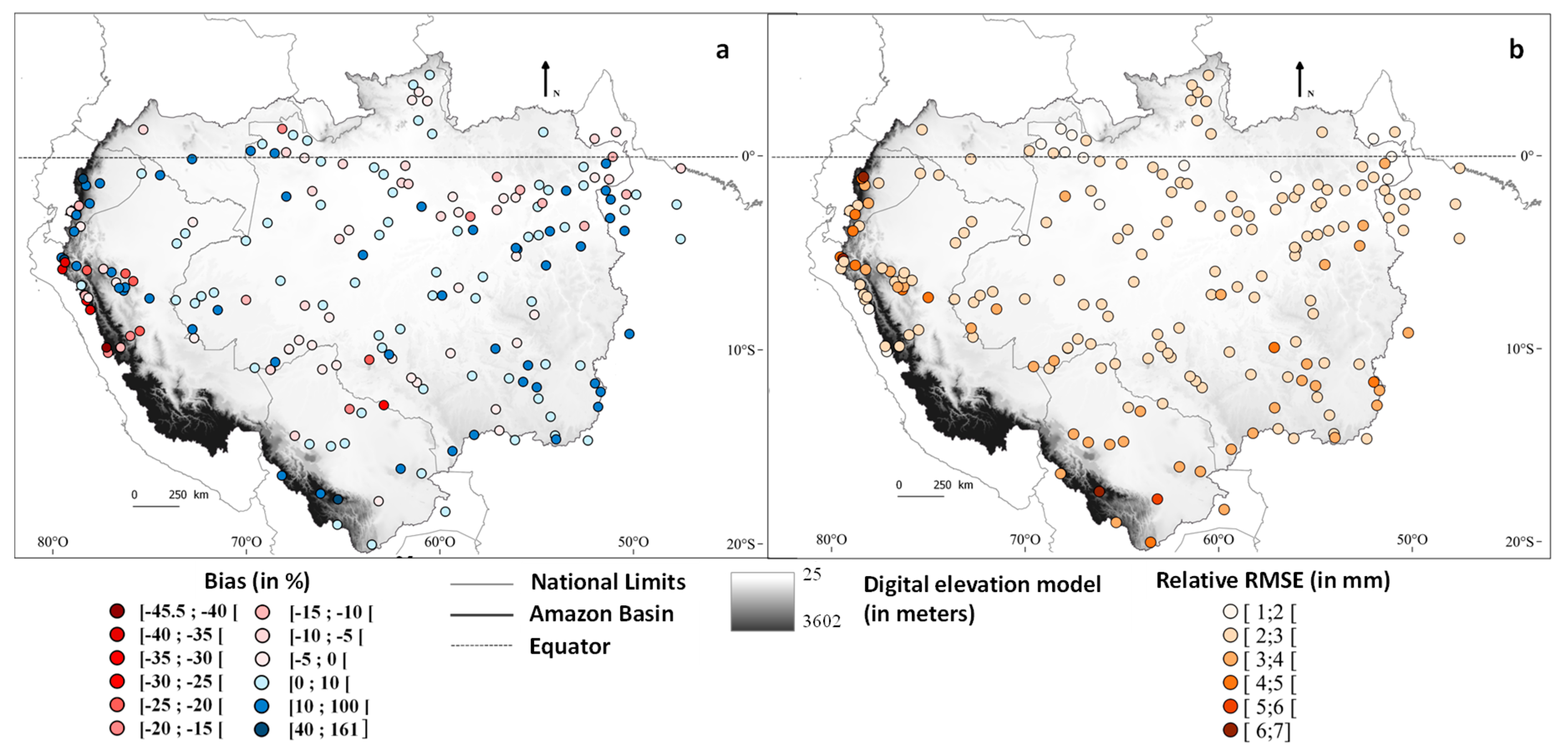
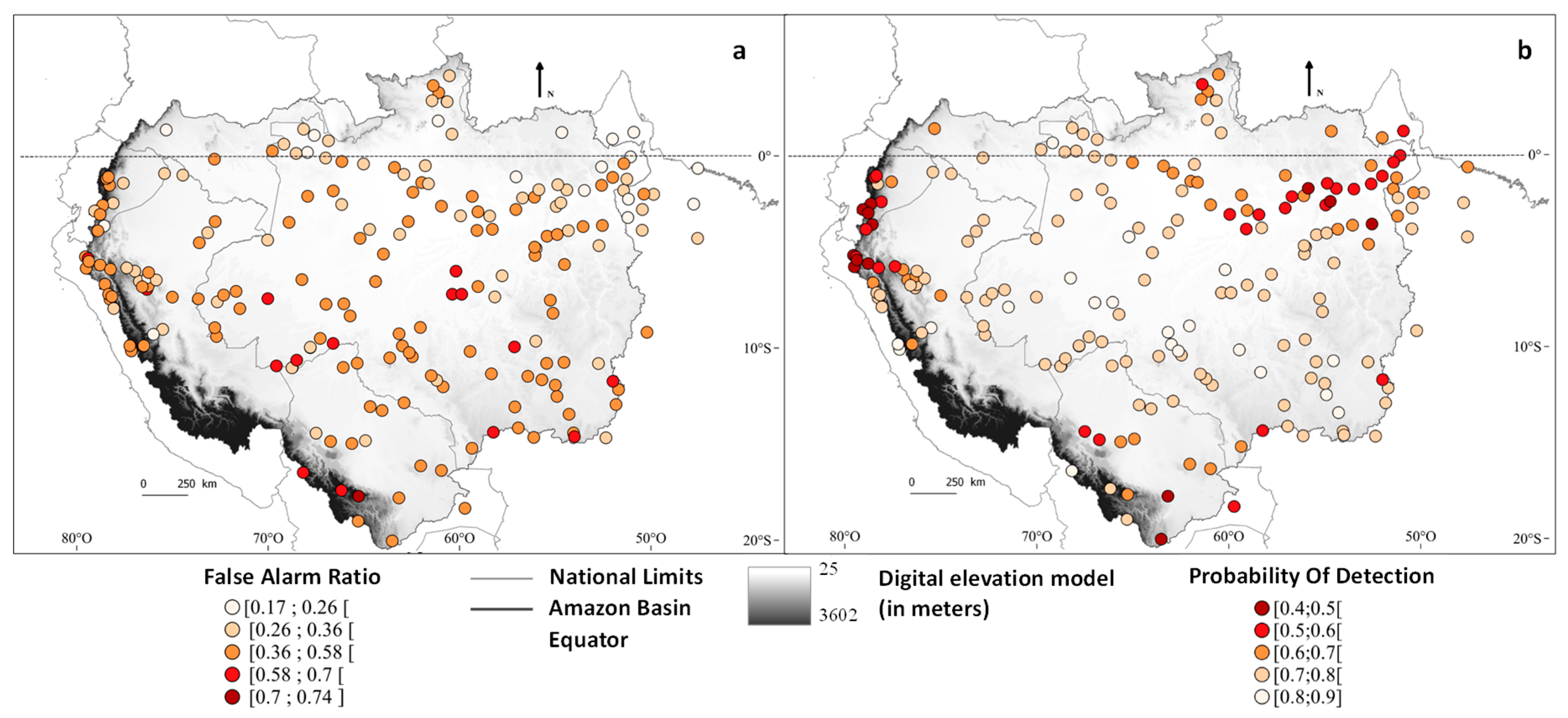
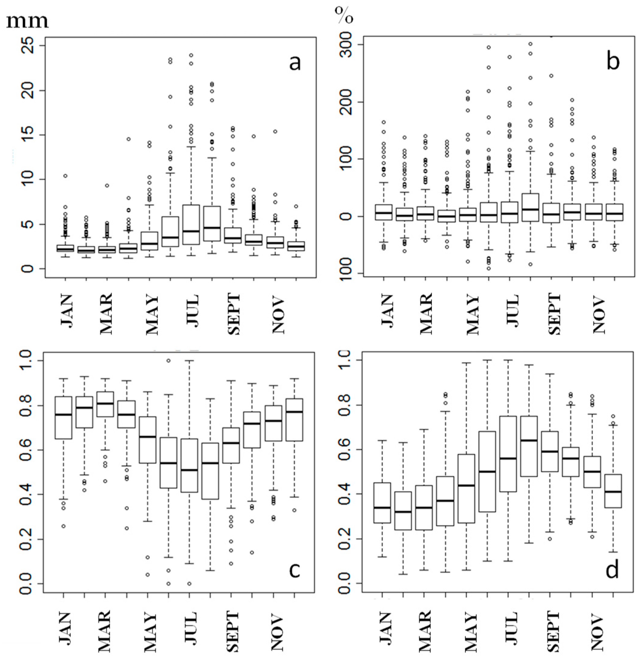
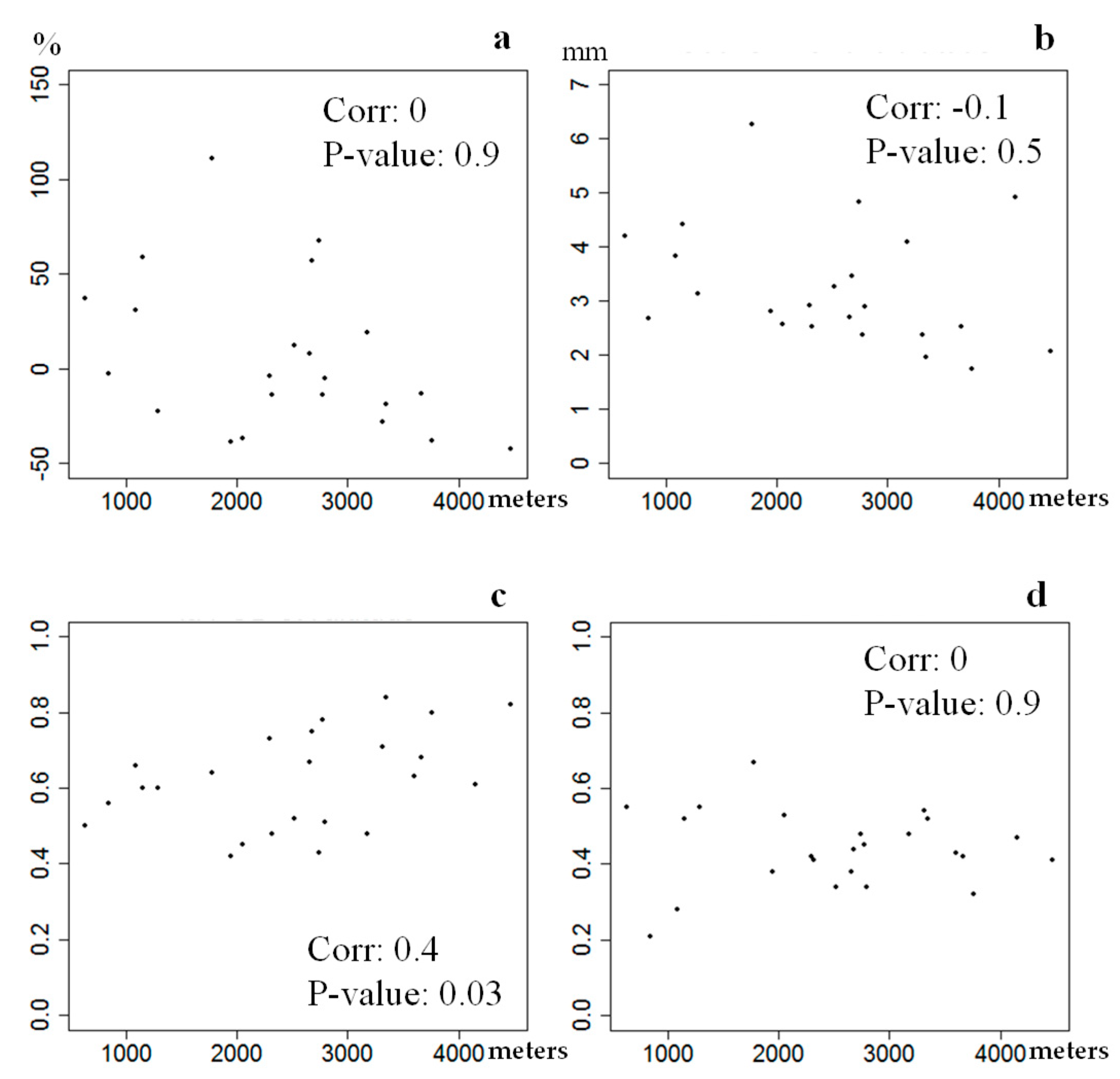
3.2. Regional and Time Analysis of TRMM 3B42 V7 Performance

At large scale, for the whole AB, 3B42 reproduces well the spatial distribution of mean daily rainfall (Figure 3a,b), with the highest rates of rainfall near the equator while rainfall decreases toward the tropics. Since the performance of 3B42 varies across the AB the statistical tools are computed at regional and annual time scale. Moreover, as in the previous section they are now computed month by month to examine whether there are any seasonal differences. The regions resulting from the spectral clustering analysis (Figure 2) may be divided into two groups: one where rainy and dry seasons alternate (Figure 7, regions northeast, south, north), and the other without pronounced dry or rainy season (Figure 7, center, west).

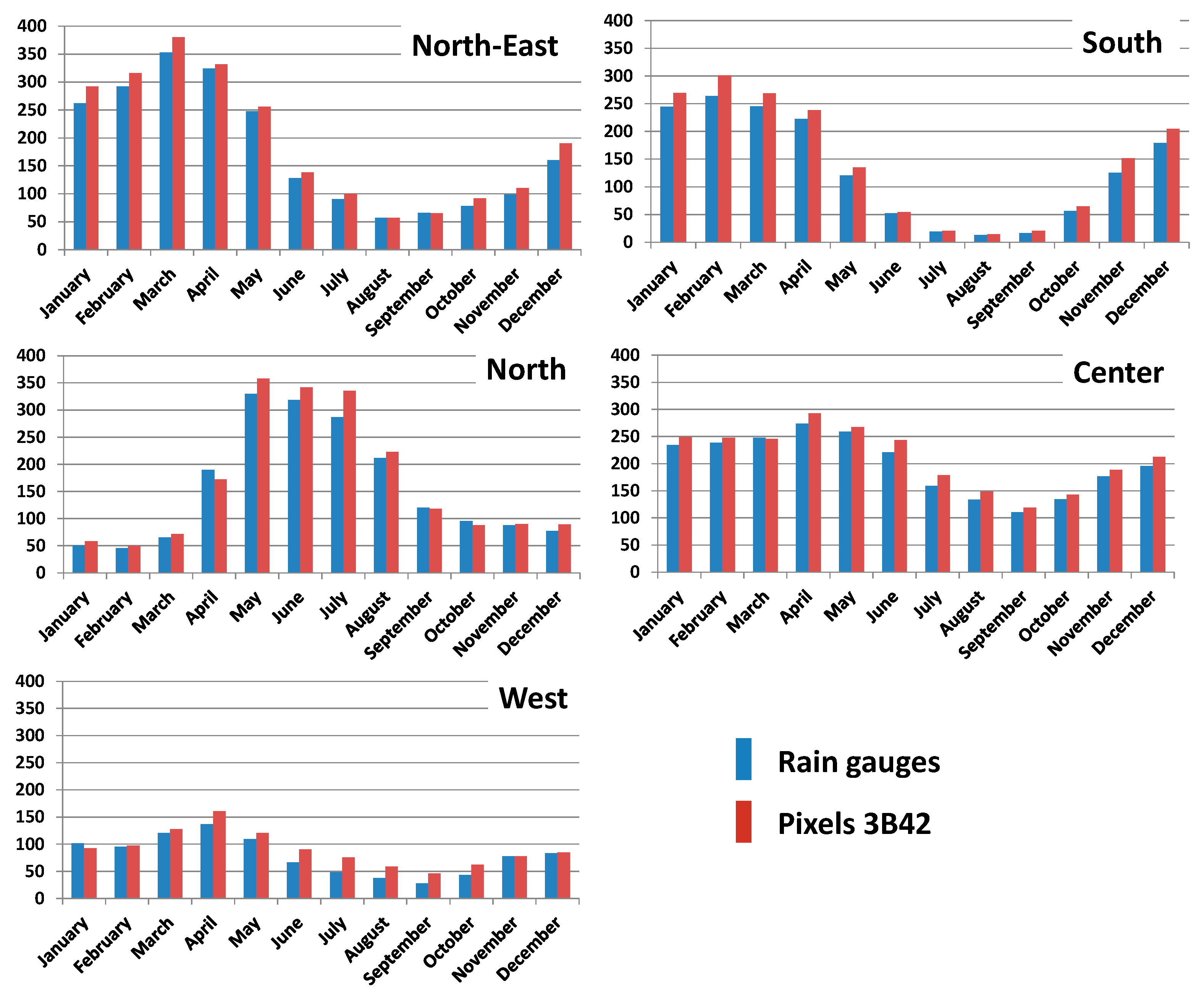
3.2.1. Annual Rainfall in the Regions

In addition to the time-averaged, global 3B42 quality assessment, observed and estimated regional mean annual rainfall and regimes have been computed for five regions within the AB. For all regions the mean annual precipitation was overestimated by 3B42 (

Table 1. Comparison between rain gauge and 3B42 mean annual rainfall (in mm), in each region of the AB. Differences are computed with respect to rain gauge mean.

Region	3B42	Rain Gauge	Difference 3B42-Rain Gauge
Northeast	2202	2140	+3%
South	1635	1536	+6%
North	1893	1873	+1%
Center	2405	2373	+1%
West	1026	967	+6%

). However, this overestimation is weak in the north and center regions, while south and west regions have the worst results with an average of 6% overestimation.

3.2.2. Regional Rainfall Regimes

Figure 7 shows a close reproduction, for all regions, of the mean annual rainfall regimes by 3B42 (despite overestimation in the total mean) with accurate distinction between rainy and dry seasons. The overestimation depends on the month and varies regionally as well: in south, north, and northeast regions rainfall is overestimated during the rainiest months, whereas in center and west regions, the strongest overestimation is observed from March to July.

Furthermore, the statistical parameters show, as for the whole Amazon (Figure 6), a contrast between rainy and dry seasons (Figure 8) with a higher occurrence of low POD and high FAR, a higher bias and RMSE during the driest months. However, that contrast presents a spatial dependence: during their respective driest months the worst bias are near by +5% for the north, below 10% for the center and the northeast and between +20 and 25% for the south and the west region. In this later region, a higher bias during the dry season is coherent with the observation of Zubieta et al. [22] in the Ecuador (until +25%) from 2003 to 2009. However, in each region during their driest months the Bias have a large range of values. On the contrary, during their rainiest months, the bias has lower range of value and the results are better in all the region. These poorer and changing results during the regional driest period, as well as the contrast with the rainiest period (which has better results), are observed for all statistical parameters here (Figure 8).

Once again, the type of rain gauge used could, in part, explain the errors and differences between the regions. Indeed, during the dry season, in the case of tipping bucket rain gauges, if the rainfall is heavy and the bucket take time to fill and tilt, a part of the rainfall can be evaporated [41,42] and not recorded while 3B42 registered this rainfall amount. Unfortunately, because of a lack of information we were not able to take it into account and understand how it may influence the results. However, the type of cloud organization in winter and the difference in spatial resolution of the two datasets [13,16] also appeared to make clear a part of the results. During the dry season, the convection is local, sparse and rainy events are scarcer than during the rainiest months especially in the southern Amazon (south of 6° S) and in the eastern equatorial part of the Amazon [43]. Then a plausible explanation would be that because of its spatial resolution, 3B42 is able to detect a rainy event while the rain gauge cannot, but conversely 3B42 may not detect an event if the convection is too shallow. Additionally, because of the low number of rainy events during the driest months, errors are relatively higher than in other seasons. Conversely, good results in the central region may be due to low seasonal rainfall contrast and deep convection. Future works will further investigate this aspect using cloud cover product as Durieux et al. [44,45] who large range of rainfall examined 10 years of three-hourly infrared data from the International Satellite Cloud Climatology Project.

The south and west regions present the worst results for all statistical parameters and all months (Figure 8a–d (ii) and (v)), consistent with Figure 4 and Figure 5. In mountainous regions (the western part of the south region and the west region), the accuracy of the estimates tends to decrease with elevation [12,16]. To investigate this issue in more detail the correlation between all the statistical parameters and the elevation was examined. The results show that only POD is slightly but significantly correlated to the elevation (Figure 9c). A possible interpretation would be that at high elevation rainy events are rarer but convective systems are well organized during the summer, which allows a good detection of the events by the satellites and POD scores higher than 0.4. The other parameters do not show a significant relationship between the elevation and the quality of 3B42 estimates, in agreement with Turko who found similar results for 3B42 estimates in the Bolivian Andes.

Some other explanation of the poor results in the Andean region could be the location of the rain gauge itself and its exposure. Indeed, in the western region and in the western part of the southern region, the stations where 3B42 overestimates rainfall are located either at the bottom of a valley or are leeward (Figure 10a,b respectively). One potential interpretation is the alteration of measurements due to evapotranspiration. Indeed, satellites measure rainfall at a higher elevation that rain gauges, then if the evaporation is important, it can avoid the precipitation to hit the ground, like in the case of virga cloud, and then cause a difference of recorded value between observations and estimations [46]. Conversely, due to the orographic effect, some precipitations can form close to the ground by advection of humid air on the hillside well exposed to the wind; in that case, the station is able to catch such precipitations, while satellites are not. Another possibility is that strong winds blow the rainfall and avoid it to enter in the rain gauges when this one are exposed to these winds. However we do not have this wind exposition information. At topographic scale, the orography also seems to explain some of 3B42 overestimation. Figure 10a presents for instance a case of stations sheltered by a mountain range. Main winds from the northwest are blocked by this rock and form a rainfall hotspot on the northern slope [18].

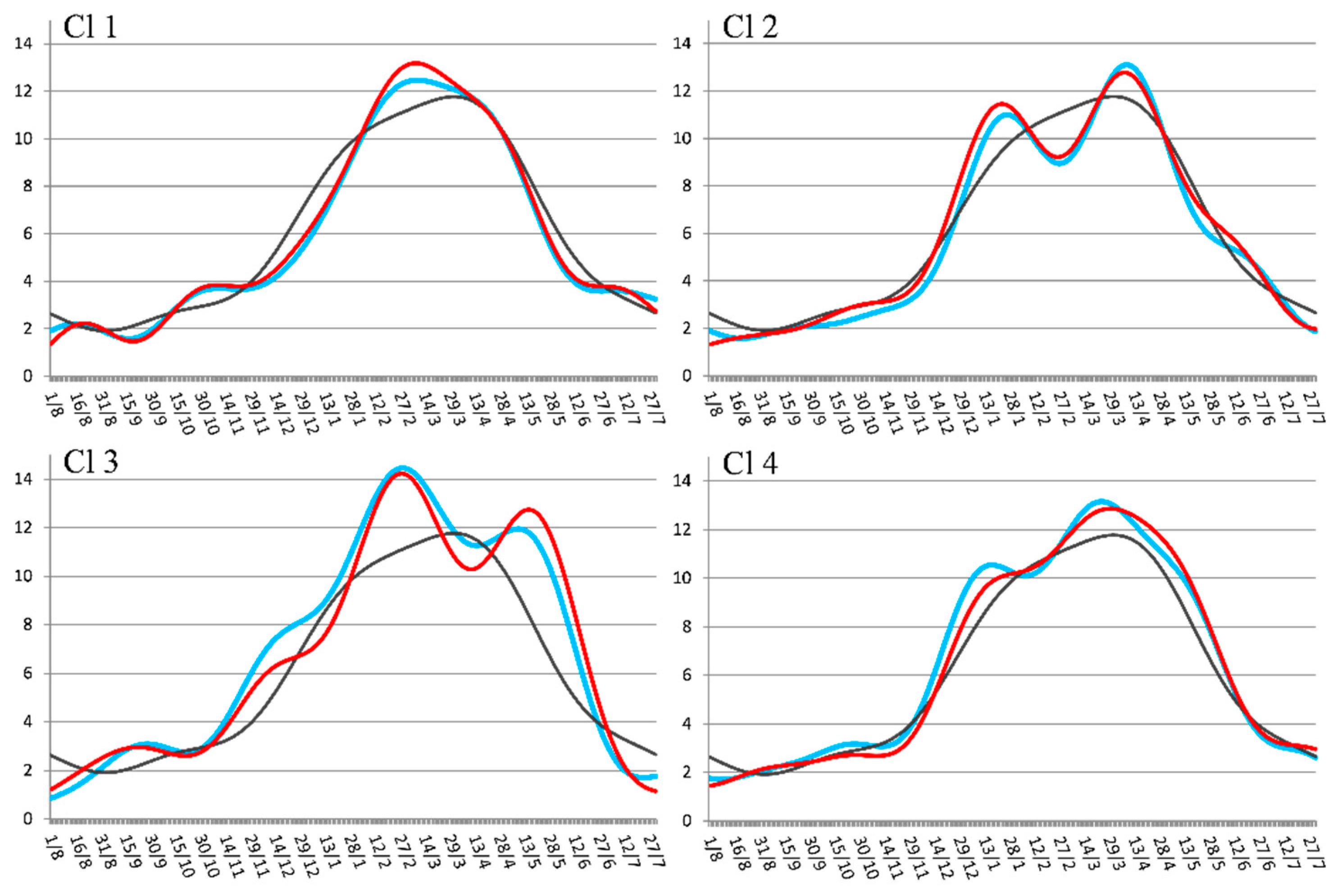
3.2.3. Regional Rainfall Sub-Regimes in the Northeastern Region of the AB

The interannual regional rainfall variability sub-regimes were first analyzed using the rain gauge network. For each region, between two and four groups of years presenting the same type of rainfall sub-regime were defined using the spectral clustering method. These sub-regimes were assumed to depict the interannual variability of regional precipitation. Hereafter we present the results for the northeastern region (Figure 2), as it contains a relatively large number of rain gauges, and good 3B42 performance.

Table 2. Years included in each rainfall sub-regime (Cl1 to Cl4) detected on the rain time series, by spectral clustering method, in the northeastern region of the AB.

Year	Cluster
2002–2003	1
2004–2005	1
2006–2007	1
2011–2012	1
2000–2001	2
2001–2002	2
2009–2010	2
2010–2011	2
2008–2009	3
1998–1999	4
1999–2000	4
2005–2006	4
2007–2008	4

shows the clusters and the years belonging to each cluster and

Table 3. Rain gauge and 3B42 mean annual rainfall (in mm) for each rainfall sub-regime of the northeastern region.

Rainfall Sub-Regime	Rain Gauge	3B42	Errors (%) of 3B42
Cl1	2181	2234	2
Cl2	2170	2261	4
Cl3	2545	2607	2
Cl4	2369	2419	2

rain gauge and 3B42 mean annual rainfall (in mm) for each rainfall sub-regime of the northeastern region. For each rainfall sub-regime, 3B42 tends to overestimate by 2 to 4% the annual precipitation (Table 3), which is coherent with the analysis of the mean regional rainfall regime (Figure 5).

Despite the overestimation in the mean annual totals, Figure 11 shows that the annual cycles of rainfall of observed and estimated precipitation are similar for the four rainfall sub-regimes in the northeastern region. The seasonal and intra-seasonal inflections of the curve are well reproduced by 3B42. In comparison with a traditional analysis of annual precipitations, this sub-regime approach shows the irregular distribution errors along the year. Furthermore, and in contrast with Figure 7a, the mismatches depend on the rainfall sub-regime and not on a specific month or period of the year. The highest overestimation of annual precipitation in Cl2 (Table 3) appears to be caused by a slight but persistent overestimation all year long (Figure 11), while the strongest overestimation between May and July in Cl3 is smoothed by underestimation during the other months of the year. Despite these differences, the reproduction of precipitation patterns by 3B42 is quite accurate.

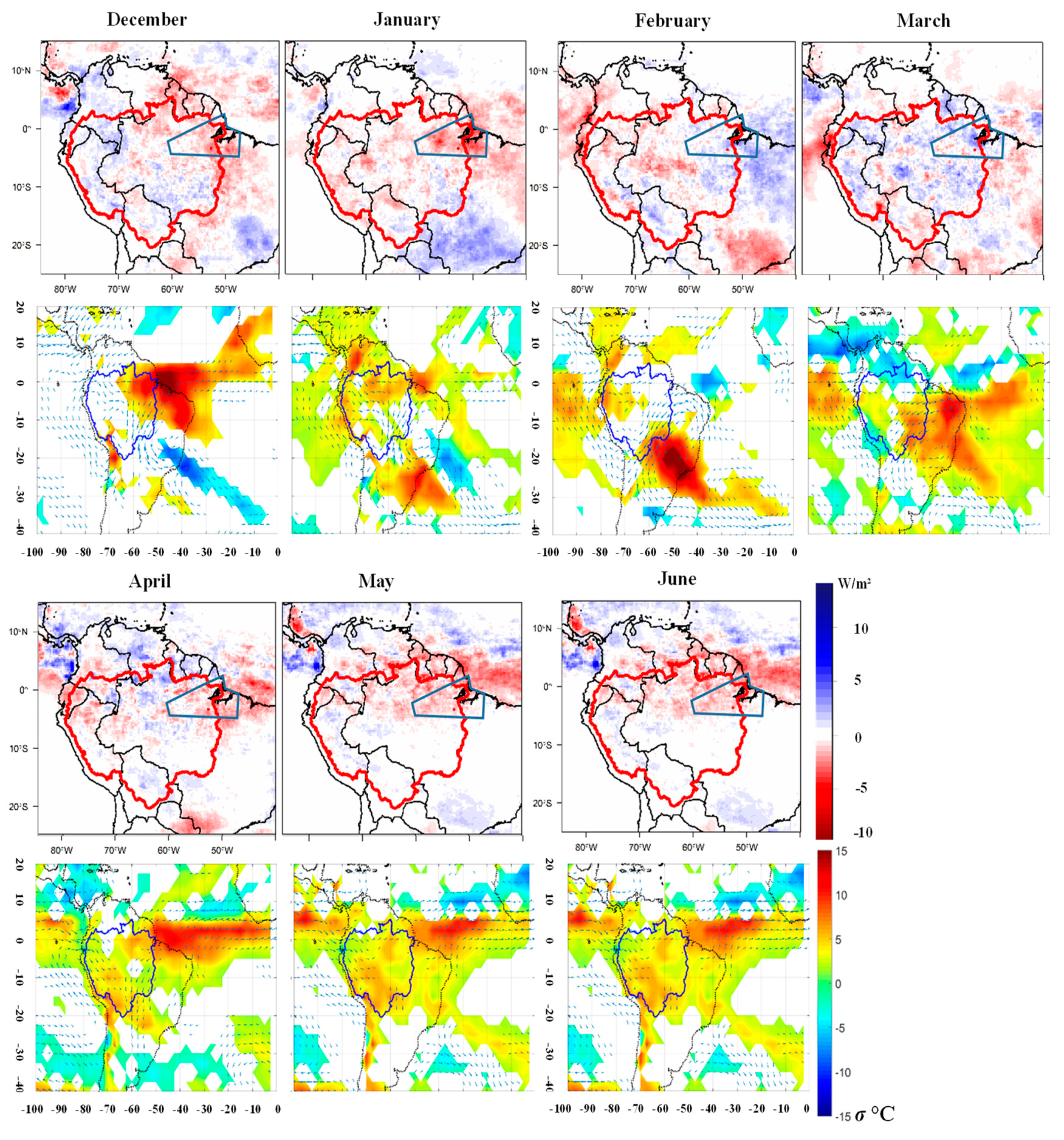
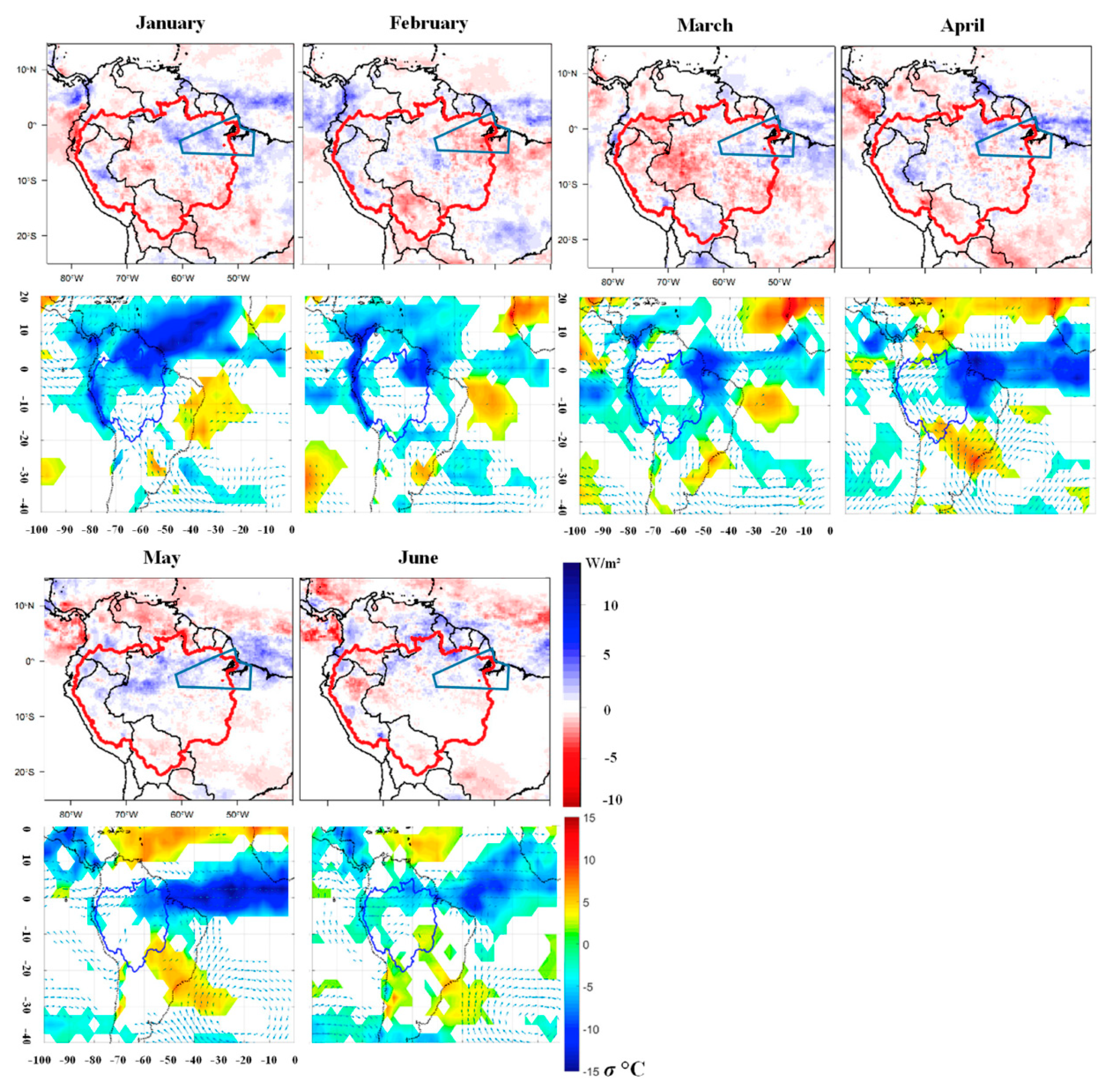
3.3. Comparisons between 3B42, Water Vapor Flux, and OLR Spatial Pattern Anomalies

Up to now, a point-to-pixel approach was used in order to validate 3B42 estimates for the AB, however, there still remains the question whether 3B42 delivers spatially coherent patterns if we consider all grid points (i.e., grid points beyond the pixels used for the comparisons with ground station).

To investigate this issue, the monthly anomalies derived from the full grid of 3B42 (hereafter 3B42 grid) were analyzed for the northeastern region. OLR anomalies were then used to confirm the spatial pattern of 3B42 grid anomalies and water vapor flux to try to explain these anomalies. Monthly anomalies of these variables correspond to the difference between the mean value of the years of the rainfall sub-regime and the mean value of the period 1998–2013 and only the significant anomalies values (higher than 1 standard deviation) are represented in Figure 12 and Figure 13. The precipitation anomalies are normalized, that is, divided by the standard deviation of the whole study period.

The analysis was performed in all the cluster sub-regimes [37], but we focus on the sub-regime Cl1 and Cl4 which are contrasted. Indeed, Cl1 has a shorter peak period than the average cycle of the region (grey line), and Cl4 on the contrary, has a longer rainfall peak (Figure 11). Furthermore, the explanations of the anomalies by the atmospheric circulation are very clear for these two clusters, which are chosen as examples. Cl3 only contains one year which can confuse the results

Figure 12 and Figure 13 show for sub-regimes Cl1 and Cl4, composite maps of normalized monthly anomalies of 3B42 grid and OLR and water vapor flux monthly anomalies. The blue polygon indicates the northeastern region within the AB. A positive (negative) OLR anomaly in warm (cold) color indicates less (more) convection and consequently, a lower (higher) probability of positive (negative) rainfall anomalies. The water vapor flux anomalies represented by vectors indicate if more or less humidity is advected to the AB; a lower (higher) transport of humidity is consistent with lower (higher) convection.

Composites for Cl1 show that 3B42 grid rainfall anomalies are in good agreement with the previous rainfall sub-regimes found at rain gauge and 3B42 pixel. The shorter rainfall peak observed in Figure 11 is in agreement with negative precipitation anomalies in the 3B42 grid in the northeastern region. These anomalies may be homogeneously distributed in the region, as in January and June, or concentrated in certain areas (e.g., in December and May). This highlights the high spatial rainfall variability and the difficulty to take it into account with the rain gauge network only. The anomalies of the 3B42 and OLR composites also are in accordance (Figure 12) and show strong negative anomalies of convection in the northeastern region in December–January and May–June (Figure 12), which is in line with a reduced peak of rainfall in this region occurring usually from December to May. The deficit of precipitation and positive OLR anomalies are consistent with the reduced and divergent water vapor flux from North Tropical Atlantic (NATL). See for instance the lack convergent water vapor fluxes in December–January and May–June over the region, while convergent fluxes are observed from February to April when enhanced precipitation is observed. The excess of rainfall in February–March, during the rainfall peak (Figure 11), appears to be linked with an area with positive rainfall (Figure 11) close to the coast that is strongly influenced by the water vapor flux from tropical ocean. These fluxes are slightly reinforced in March and may explain the enhanced rainfall during this period of the year. Another feature that appears using the 3B42 grid is the opposed inland and coastal anomalies inside the region (e.g., in March and April, Figure 12).

The precipitation anomalies in the 3B42 grid composites of the rainfall sub-regime Cl4 also highlight the importance of the local scale compared to the regional scale. Indeed, during the longer and higher than usual rainy peak of Cl4, with strong surpluses of precipitation in January and from March to June (Figure 11), rainfall anomalies appear in the 3B42 grid composites but with an inhomogeneous spatial distribution (Figure 13). In contrast, in February the slight rainfall deficits in rainfall sub-regime 3B42 pixel (Figure 11) also appears in the 3B42 grid, but the latter have a more spatial homogeneous pattern. The positive rainfall anomaly is connected to negative OLR anomalies (Figure 12) on the northeast of the AB and on the Atlantic ITCZ in January and from March to June. The convection increase is related to the convergence in the northeastern region between water vapor flux anomalies from the west, the north and the southeast, as well as a weaker than usual export of humidity by the low-level jet to the La Plata Basin. On the contrary, in February even if strong convection is present on the Northeast AB region the water vapor fluxes are reduced which is coherent with the rainfall deficits of 3B42 grid in this region in years where Cl4 dominates.

4. Conclusions

The 3B42 daily precipitation product is an incredibly valuable product as it provides spatial rainfall information for the whole AB, where the access to ground observed data is particularly complicated. However, as they are estimated, some bias and errors exist that need to be assessed. The evaluation of the 3B42 quality was done by means of quantitative (mean daily rainfall, bias, relative RMSE) and categorical statistics (POD and FAR), considering daily data in the whole basin. These statistical parameters showed monthly differences with a contrast between the dry and rainy period. This last one presents the better results. In relation to these intra-annual contrasts, we focused our evaluation on regional rainfall regimes and sub-regimes which have not been shown in any previous studies The average bias is +7% (overestimation), but large errors ranging from −45% to +161% are observed in the Andean regions. 3B42 performs better in the detection of rainy events than in the quantitative estimation of rainfall. Also, as observed in previous studies and as shown by all the statistics, 3B42 performs better in the lowlands of the AB than in mountainous regions of the Andes. However this work highlights differences within the high areas: in the northern (Ecuador) and southern Andes (Bolivia) 3B42 tends to overestimate precipitation, whereas in central Andes (Peru) rainfall is underestimated. Furthermore, no correlation is found between the elevation of the stations and the results of the statistical parameters. Warm clouds are frequently assumed to be a factor of the difference measured between observed and estimated precipitations. However, others phenomena in AB can also cause differences between observed and estimated data. Indeed, overestimation by 3B42 can results from the capacity of satellite to measure precipitation at high elevation, while the evaporation avoids this same precipitation to hit the ground and then, the rain gauges. Underestimations by 3B42 could depend on orography with a low capacity to detect orographic rainfall forming close to the ground on hillside exposed to the main wind, while the rain gauge succeeds in catching it. Furthermore, we assume that further evaluation can be done by considering several threshold values to determine the occurrence of a precipitation event (here, 0.1mm) to check if underestimation depends on such threshold.

The ability of 3B42 to accurately replicate annual rainfall regimes in the different AB regions was also used as a tool to assess its quality. There is generally a good agreement between regional regimes derived either from rain gauge or 3B42. However, in each region, the performance of 3B42 is lower during the drier period than during the rainy period. That could be partially explained by the difference in spatial resolution of the two datasets (the sparse occurrence of rainfall not being measured by the rain gauges but being captured by 3B42). Also, during the drier period, rainy events are scarcer and the relative error may be larger.

Rainfall sub-regimes from the rain gauge and those from the 3B42 pixels were compared and are in good agreement in the northeastern region, despite an overestimation of 2 to 4% of annual rainfall. The seasonal and intra-seasonal behavior is reproduced well. It is worth noting that over or underestimation of 3B42 pixel do not depend on the months or the season, and differ between the rainfall sub-regimes.

Finally, the adequacy between observed and estimated rainfall sub-regimes were compared looking at the whole northeast grid. Generally, both are in good agreement. However, it can be noted that sometimes precipitations anomalies are not homogeneous in the northeastern region, for instance with differences between inland and coastal sectors. That underlines a high spatial rainfall variability that is difficult to take into account with a rain gauge network only, and highlights the importance of spatially refined data such as 3B42. Spatial and time accuracy of 3B42 grid anomalies are coherent with the water vapor flux and OLR anomalies, despite their different resolutions.

At a daily scale, in most parts of AB, 3B42 provides an exhaustive and quite good precipitation dataset. This higher quantity of information with satisfactory quality emphasizes intraregional precipitation distribution, especially between coastal (often influenced by sea breeze front) and inland sectors. Nevertheless, when using 3B42 for the AB, data should be used with caution in the dry season or in mountainous regions. Beyond these aspects, the upcoming data homogenization between 3B42 and the recent Global Precipitation Measurement Mission will provide a longer and improved rainfall estimated time series.

References

1. Meinke, H.; Stone, R.C. Seasonal and Inter-Annual Climate Forecasting: The New Tool for Increasing Preparedness to Climate Variability and Change in Agricultural Planning and Operations. Clim. Chang. 2005, 70, 221–253. [Google Scholar] [CrossRef]
2. Arvor, D. Etude par Télédétection de la Dynamique du soja et de L’impact des Précipitations sur les Productions au Mato Grosso (Brésil). Thèse de Doctorat, Université Rennes 2, Rennes, France, 2009. [Google Scholar]
3. Brondizio, E.S.; Moran, E.F. Human dimensions of climate change: The vulnerability of small farmers in the Amazon. Philos. Trans. R. Soc. Lond. B Biol. Sci. 2008, 363, 1803–1809. [Google Scholar] [CrossRef] [PubMed]
4. Coomes, O.T.; Lapointe, M.; Templeton, M.; List, G. Amazon river flow regime and flood recessional agriculture: Flood stage reversals and risk of annual crop loss. J. Hydrol. 2016, 539, 214–222. [Google Scholar] [CrossRef]
5. Liebmann, B.; Allured, D. Daily precipitation grids for South America. Bull. Am. Meteorol. Soc. 2005, 86, 1567. [Google Scholar] [CrossRef]
6. Dubreuil, V.; Arvor, D.; Ronchail, J. Potentialités des données TRMM pour la spatialisation des précipitations au Mato Grosso, Brésil. In Proceedings of the XXe Colloque de l’Association Internationale de Climatologie, Carthage, Tunisie, 3–9 September 2007; pp. 210–215. [Google Scholar]
7. Ronchail, J.; Cochonneau, G.; Molinier, M.; Guyot, J.-L.; De Miranda Chaves, A.G.; Guimarães, V.; de Oliveira, E. Interannual rainfall variability in the Amazon basin and sea-surface temperatures in the equatorial Pacific and the tropical Atlantic Oceans. Int. J. Climatol. 2002, 22, 1663–1686. [Google Scholar] [CrossRef] [Green Version]
8. Delahaye, F. Analyse Comparative des Différents Produits Satellitaires D’estimation des Précipitations en Amazonie Brésilienne. Thèse de Doctorat, Université Rennes 2, Rennes, France, 2013. [Google Scholar]
9. Cai, Y.; Jin, C.; Wang, A.; Guan, D.; Wu, J.; Yuan, F.; Xu, L. Spatio-temporal analysis of the accuracy of tropical multisatellite precipitation analysis 3B42 precipitation data in mid-high latitudes of China. PLoS ONE 2015, 10, e0120026. [Google Scholar] [CrossRef] [PubMed]
10. Guo, R.; Liu, Y. Evaluation of Satellite Precipitation Products with Rain Gauge Data at Different Scales: Implications for Hydrological Applications. Water 2016, 8, 281. [Google Scholar] [CrossRef]
11. Tian, Y.; Peters-Lidard, C.D.; Choudhury, B.J.; Garcia, M. Multitemporal analysis of TRMM-based satellite precipitation products for land data assimilation applications. J. Hydrometeorol. 2007, 8, 1165–1183. [Google Scholar] [CrossRef]
12. Zulkafli, Z.; Buytaert, W.; Onof, C.; Manz, B.; Tarnavsky, E.; Lavado, W.; Guyot, J.L. A comparative performance analysis of TRMM 3B42 (TMPA) versions 6 and 7 for hydrological applications over Andean–Amazon River basins. J. Hydrometeorol. 2014, 15, 581–592. [Google Scholar] [CrossRef]
13. Salio, P.; Hobouchian, M.P.; Skabar, Y.G.; Vila, D. Evaluation of high-resolution satellite precipitation estimates over southern South America using a dense rain gauge network. Atmos. Res. 2015, 163, 146–161. [Google Scholar] [CrossRef]
14. Dinku, T.; Connor, S.J.; Ceccato, P. Comparison of CMORPH and TRMM-3B42 over Mountainous Regions of Africa and South America. In Satellite Rainfall Applications for Surface Hydrology; Gebremichael, M., Hossain, F., Eds.; Springer: Dordrecht, The Netherlands, 2010; pp. 193–204. ISBN 978-90-481-2915-7. [Google Scholar]
15. Mohd Zad, S.; Zulkafli, Z.; Muharram, F. Satellite Rainfall (TRMM 3B42-V7) Performance Assessment and Adjustment over Pahang River Basin, Malaysia. Remote Sens. 2018, 10, 388. [Google Scholar] [CrossRef]
16. Thiemig, V.; Rojas, R.; Zambrano-Bigiarini, M.; Levizzani, V.; De Roo, A. Validation of satellite-based precipitation products over sparsely gauged African river basins. J. Hydrometeorol. 2012, 13, 1760–1783. [Google Scholar] [CrossRef]
17. Bookhagen, B.; Strecker, M.R. Orographic barriers, high-resolution TRMM rainfall, and relief variations along the eastern Andes. Geophys. Res. Lett. 2008, 35, L06403. [Google Scholar] [CrossRef]
18. Espinoza, J.C.; Chavez, S.; Ronchail, J.; Junquas, C.; Takahashi, K.; Lavado, W. Rainfall hotspots over the southern tropical Andes: Spatial distribution, rainfall intensity, and relations with large-scale atmospheric circulation. Water Resour. Res. 2015, 51, 3459–3475. [Google Scholar] [CrossRef]
19. Paccini, L.; Espinoza, J.C.; Ronchail, J.; Segura, H. Intra-seasonal rainfall variability in the Amazon basin related to large-scale circulation patterns: A focus on western Amazon-Andes transition region: Intra-seasonal rainfall variability in western Amazon. Int. J. Climatol. 2018, 38, 2386–2399. [Google Scholar] [CrossRef]
20. Getirana, A.C.; Espinoza, J.C.V.; Ronchail, J.; Rotunno Filho, O.C. Assessment of different precipitation datasets and their impacts on the water balance of the Negro River basin. J. Hydrol. 2011, 404, 304–322. [Google Scholar] [CrossRef]
21. Buarque, D.C.; de Paiva, R.C.D.; Clarke, R.T.; Mendes, C.A.B. A comparison of Amazon rainfall characteristics derived from TRMM, CMORPH and the Brazilian national rain gauge network. J. Geophys. Res. 2011, 116. [Google Scholar] [CrossRef] [Green Version]
22. Zubieta, R.; Getirana, A.; Espinoza, J.C.; Lavado, W. Impacts of satellite-based precipitation datasets on rainfall–runoff modeling of the Western Amazon basin of Peru and Ecuador. J. Hydrol. 2015, 528, 599–612. [Google Scholar] [CrossRef]
23. Zhou, J.; Lau, K.M. Does a Monsoon Climate Exist over South America? J. Clim. 1998, 11, 1020–1040. [Google Scholar] [CrossRef]
24. Marengo, J.A.; Liebmann, B.; Kousky, V.E.; Filizola, N.P.; Wainer, I.C. Onset and End of the Rainy Season in the Brazilian Amazon Basin. J. Clim. 2001, 14, 833–852. [Google Scholar] [CrossRef] [Green Version]
25. Wang, H.; Fu, R. Cross-Equatorial Flow and Seasonal Cycle of Precipitation over South America. J. Clim. 2002, 15, 1591–1608. [Google Scholar] [CrossRef]
26. Vera, C.; Baez, J.; Douglas, M.; Emmanuel, C.B.; Marengo, J.; Meitin, J.; Nicolini, M.; Nogues-Paegle, J.; Paegle, J.; Penalba, O.; et al. The South American Low-Level Jet Experiment. Bull. Am. Meteorol. Soc. 2006, 87, 63–77. [Google Scholar] [CrossRef]
27. Figueroa, S.N.; Nobre, C.A. Precipitation distribution over central and western tropical South America. Climanalise 1990, 5, 36–45. [Google Scholar]
28. Marengo, J.A. Interannual variability of surface climate in the Amazon basin. Int. J. Climatol. 1992, 12, 853–863. [Google Scholar] [CrossRef]
29. Espinoza Villar, J.C.; Ronchail, J.; Guyot, J.L.; Cochonneau, G.; Naziano, F.; Lavado, W.; De Oliveira, E.; Pombosa, R.; Vauchel, P. Spatio-temporal rainfall variability in the Amazon basin countries (Brazil, Peru, Bolivia, Colombia, and Ecuador). Int. J. Climatol. 2009, 29, 1574–1594. [Google Scholar] [CrossRef] [Green Version]
30. Michot, V.; Dubreuil, V.; Roncahil, J.; Lucio, P.S. Constitution et analyse critique d’une base de données spatiale pour l’étude des saisons des pluies dans le bassin amazonien. In Proceedings of the ENVIBRAS 2014 Environnement et Géomatique: Approches Comparées France—Brésil, Rennes, France, 12–15 November 2014; pp. 237–244. [Google Scholar]
31. Michot, V.; Arvor, D.; Ronchail, J.; Corpetti, T.; Jégou, N.; Lucio, P.S.; Dubreuil, V. Validation and reconstruction of rain gauge-based daily time series for the entire Amazon basin. Theor. Appl. Climatol. 2018. under review. [Google Scholar]
32. Huffman, G.J.; Bolvin, D.T. TRMM and Other Data Precipitation Data Set Documentation 2015. Available online: https://pmm.nasa.gov/sites/default/files/document_files/3B42_3B43_doc_V7.pdf (accessed on 10 August 2015).
33. Liebmann, B.; Smith, A.C. Description of a complete (interpolated) outgoing longwave radiation dataset. Bull. Am. Meteorol. Soc. 1996, 77, 1275–1277. [Google Scholar]
34. Kalnay, E.; Kanamitsu, M.; Kistler, R.; Collins, W.; Deaven, D.; Gandin, L.; Iredell, M.; Saha, S.; White, G.; Woollen, J.; et al. The NCEP/NCAR 40-year reanalysis project. Bull. Am. Meteorol. Soc. 1996, 77, 437–471. [Google Scholar] [CrossRef]
35. Peixoto, J.P.; Oort, A.H. Physics of Climate; American Institute of Physics: New York, NY, USA, 1992; 520p, ISBN1 978-0-88318-711-1. ISBN2 978-0-88318-712-8. [Google Scholar]
36. Scheel, M.L.M.; Rohrer, M.; Huggel, C.; Santos Villar, D.; Silvestre, E.; Huffman, G.J. Evaluation of TRMM Multi-satellite Precipitation Analysis (TMPA) performance in the Central Andes region and its dependency on spatial and temporal resolution. Hydrol. Earth Syst. Sci. 2011, 15, 2649–2663. [Google Scholar] [CrossRef] [Green Version]
37. Michot, V. Analyse Spatiale et Temporelle de la Variabilité des Régimes de Précipitations dans le Bassin Amazonien. Ph.D. Thesis, Université Bretagne-Loire, Rennes 2, Rennes, France, 2017. [Google Scholar]
38. Camps-Valls, G.; Bruzzone, L. Kernel Methods for Remote Sensing Data Analysis; John Wiley & Sons: Chichester, UK, 2009; ISBN 978-0-470-74899-2. [Google Scholar]
39. Barbosa Santos, E.B. Modelagem estatística e atribuições dos eventos de precipitação extrema na Amazônia brasileira. In Statistical Modeling and Attributions of Extreme Precipitation Events in the Brazilian Amazon; Universidade Federal do Rio Grande: Do Norte Natal, Brazil, 2015. [Google Scholar]
40. Delahaye, F.; Kirstetter, P.-E.; Dubreuil, V.; Machado, L.A.; Vila, D.A.; Clark, R. A consistent gauge database for daily rainfall analysis over the Legal Brazilian Amazon. J. Hydrol. 2015, 527, 292–304. [Google Scholar] [CrossRef]
41. Groisman, P.Y.; Legates, D.R. The Accuracy of United States Precipitation Data. Bull. Am. Meteorol. Soc. 1994, 75, 215–227. [Google Scholar] [CrossRef] [Green Version]
42. Wang, J.; Fisher, B.L.; Wolff, D.B. Estimating Rain Rates from Tipping-Bucket Rain Gauge Measurements. J. Atmos. Oceanic Technol. 2008, 25, 43–56. [Google Scholar] [CrossRef] [Green Version]
43. Fu, R.; Zhu, B.; Dickinson, R.E. How Do Atmosphere and Land Surface Influence Seasonal Changes of Convection in the Tropical Amazon? J. Clim. 1999, 12, 1306–1321. [Google Scholar] [CrossRef]
44. Durieux, L. Etude des Relations entre les Caractéristiques Géographiques de la Surface et les Nuages Convectifs dans la Région de L’arc de Déforestation en Amazonie. Ph.D. Thesis, Université de Provence, UFR Des Sciences Géographiques et de L’aménagement, Aix-Marseille, France, 2002. [Google Scholar]
45. Durieux, L. The impact of deforestation on cloud cover over the Amazon arc of deforestation. Remote Sens. Environ. 2003, 86, 132–140. [Google Scholar] [CrossRef]
46. Wang, Z.; Sassen, K. Cloud Type and Macrophysical Property Retrieval Using Multiple Remote Sensors. J. Appl. Meteorol. 2001, 40, 1665–1682. [Google Scholar] [CrossRef]
Figure 1. Pattern of the Intertropical Convergence Zone (ITCZ), South Atlantic Convergence Zone (SACZ), South American Low Level Jet (SALLJ) core and northeast and southeast wind trades during the South American Monsoon System from December to February (DJF). Source: V. Michot.
Remotesensing 10 01879 g001
Figure 2. Rain gauge network used as ground reference (205 stations with daily data from 1998 to 2013). The colors of the stations and the labels allow identifying the climatic regions with similar rainfall regimes [33,36].
Remotesensing 10 01879 g002
Figure 3. Spatial distribution of (a) mean daily rainfall per rain gauge (b) mean daily rainfall in the nearest pixel 3B42 of the rain gauge. Both are expressed in millimeters per day. The average is computed on the 1998–2013 period.
Remotesensing 10 01879 g003
Figure 4. Spatial distribution of (a) 3B42 Bias in percent between estimated and observed rainfall, and (b) 3B42 Relative RMSE, in millimeters per day. Both are calculated from 2000 to 2013 at daily time scale.
Remotesensing 10 01879 g004
Figure 5. Spatial distribution of (a) the probability of detection and (b) the false alarm ratio. Both are calculated from 2000 to 2013 at daily time scale.
Remotesensing 10 01879 g005
Figure 6. (a) Relative RMSE (in mm), (b) bias (in mm), (c) POD, and (d) FAR of 3B42, at daily time scale for each month, calculated from 2000 to 2013 at daily time scale.
Remotesensing 10 01879 g006
Figure 7. Annual rainfall regimes of the different regions defined in Figure 2 for the AB. The x-axis represents each month of the year, y-axis represents the rainfall in millimeters per month. Blue bars represent the observed rainfall and red ones the estimated rainfall.
Remotesensing 10 01879 g007
Figure 8. (a) Relative RMSE (in mm), (b) bias (in mm), (c) POD, and (d) FAR of 3B42, at daily scale for each month of the year for the five regions: (i) the northeast, (ii) south, (iii) north, (iv) center, (v) west regions.
Remotesensing 10 01879 g008
Figure 9. Correlation between elevation and (a) bias, in %; (b) relative RMSE, in mm; (c) POD; and (d) FAR in the region west. The x-axis represents the elevation (in meters), y-axis represents the score of each statistic.
Remotesensing 10 01879 g009
Figure 10. (a,b) location of rain gauges with shelter situation and overestimation (in mm) by 3B42. The white arrow represent the main wind in the region of Bolivian rainfall hotspot [18].
Remotesensing 10 01879 g010
Figure 11. Rainfall sub-regimes Cl1 to Cl4, in the northeastern region of AB from rain gauge (blue line), 3B42 pixel (red line), and mean annual regime of the region from rain gauge (grey line).
Remotesensing 10 01879 g011
Figure 12. Monthly composite maps of 3B42 grid normalized monthly anomalies (top) and OLR and water vapor flux monthly significant anomalies (bottom). Anomalies are computed based on cluster Cl1 years in the northeastern region. The blue polygon represents the northeastern region of the AB.
Remotesensing 10 01879 g012
Figure 13. Monthly composite maps of 3B42 grid normalized monthly anomalies (top) and OLR and water vapor flux monthly significant anomalies (bottom). Anomalies are computed based on cluster Cl4 years in the northeastern region. The blue polygon represents the northeastern region of the AB.
Remotesensing 10 01879 g013