Abstract
Recent developments in remote sensing (RS) technology have made several sources of auxiliary data available to support forest inventories. Thus, a pertinent question is how different sources of RS data should be combined with field data to make inventories cost-efficient. Hierarchical model-based estimation has been proposed as a promising way of combining: (i) wall-to-wall optical data that are only weakly correlated with forest structure; (ii) a discontinuous sample of active RS data that are more strongly correlated with structure; and (iii) a sparse sample of field data. Model predictions based on the strongly correlated RS data source are used for estimating a model linking the target quantity with weakly correlated wall-to-wall RS data. Basing the inference on the latter model, uncertainties due to both modeling steps must be accounted for to obtain reliable variance estimates of estimated population parameters, such as totals or means. Here, we generalize previously existing estimators for hierarchical model-based estimation to cases with non-homogeneous error variance and cases with correlated errors, for example due to clustered sample data. This is an important generalization to take into account data from practical surveys. We apply the new estimation framework to case studies that mimic the data that will be available from the Global Ecosystem Dynamics Investigation (GEDI) mission and compare the proposed estimation framework with alternative methods. Aboveground biomass was the variable of interest, Landsat data were available wall-to-wall, and sample RS data were obtained from an airborne LiDAR campaign that produced simulated GEDI waveforms. The results show that generalized hierarchical model-based estimation has potential to yield more precise estimates than approaches utilizing only one source of RS data, such as conventional model-based and hybrid inferential approaches.
1. Introduction
For several reasons, society’s interest in forests and forestry is increasing. Forests play a key role in ambitions to mitigate climate change through moving from fossil-based economies to bio-based economies. They provide a long list of ecosystem services, including human recreational and economic uses. As a result, there is an increasing worldwide need for information about the state and change of forest resources and forest environmental conditions. One important example is the United Nations’ Framework Convention on Climate Change (UNFCCC), which has become an important driver of forest inventory development since it highlights that forests are potentially huge sources or sinks of carbon dioxide and, thus, the agreements under UNFCCC require recurrent reporting of forest carbon pool changes [1]. Another example is the Forest Europe process, which relies on forest information for promoting sustainable management of European forests [2].
A major challenge is to develop methods to collect forest information cost-efficiently, without sacrificing information quality. Typically, National Forest Inventories (NFIs) based on field sample plots provide forest information at regional and national level. However, the ongoing development of earth observation technologies is rapidly improving, and the scope, quality and availability of the data provided offer substantial new possibilities for forest inventories e.g., [3]. Over the last few decades, several studies have been conducted where remote sensing (RS) and field data have been combined in order to enhance the precision of large-scale field based inventories, or to make forest surveys feasible in remote areas where field sampling is very costly.
When conducting a forest inventory, RS data can be incorporated at either the design stage or the estimation stage. At the design stage, RS data can be used for stratification e.g., [4], unequal probability sampling e.g., [5], or balanced sampling e.g., [6]. To utilize RS data in the estimation stage, either model-based inference [7,8,9], or model-assisted estimation including post-stratification [10], i.e., design-based inference, can be applied.
The vast availability of RS data also opens new possibilities for improving estimation efficiency by using combinations of several sources of RS data. While this can be achieved straightforwardly in the case of model-assisted estimation following established sampling theory e.g., [5,11,12,13], this issue has been less explored for model-based inference for the case when auxiliary data are not available for the entire population. An important case is when wall-to-wall RS data (or a large sample) are complemented by a (sparse) sample of RS data that are strongly correlated with the forest attribute variable of interest. While several studies have utilized this type of combination of RS data for model-based inference e.g., [14,15,16], first steps towards a rigid statistical framework for this type of surveys were taken by Saarela et al. [17] and Holm et al. [18]. The current study is a generalization and expansion of those studies. The proposed technique has been termed hierarchical model-based estimation (ibid.) since in a typical case the data sources are nested. Commonly, the ambition is to utilize wall-to-wall (or a large sample of) RS data for the inference about population characteristics within a large study area. Since field data are expensive or may not be possible to obtain from all parts of the area, a sample of RS data is selected, and a model linking the study variable (from field plots) with sampled RS data is established. A key issue in hierarchical model-based estimation is that this model must provide precise predictions of the variable of interest. Thus, the sampled RS data should provide more accurate model predictions than the RS data available wall-to-wall. For example, in a biomass survey the wall-to-wall RS data might be obtained from the Landsat satellite and the sampled RS data from airborne laser scanning cf. [19]. Model predictions across the sampled set of RS data are used for estimating a second model, linking the variable of interest with wall-to-wall RS data. The latter model is used for the model-based inference, but in the uncertainty assessment both modeling steps must be accounted for [17,18,20].
Hierarchical model-based estimation can be used also in cases where data are not nested, as an approach to make use of a sparse network of existing field data. In this case a small (possibly purposive) sample of RS data is selected to link field data with a large sample of RS data, or RS data available wall-to-wall. This approach was pioneered by Boudreau et al. [14] and Nelson et al. [15], who used a combination of the Portable Airborne Laser System (PALS) and data from ICESat/GLAS for estimating aboveground biomass (AGB) in Québec, Canada. A similar approach was applied in a study by Neigh et al. [16] for assessment of forest carbon stock across the entire boreal forest region. However, these studies ignore parts of the models’ contribution to the overall uncertainty of the biomass estimators. In Saarela et al. [17] it was shown that the studies might have underestimated the variance by up to 70%. However, the study by Saarela et al. [17] was conducted under simplifying assumptions, such as assuming all samples being conducted through simple random sampling and assuming that all models involved had homogeneous residual variance.
The main objective of this study is to generalize the existing estimators for hierarchical model-based estimation so that this estimation method can be applied also in cases when the model errors have non-homogeneous variance and cases where the errors are correlated, for example due to clustered sampled data. A further objective is to compare the proposed estimation method with existing methods, using data from study sites in the USA that mimic the type of data that will be available from the Global Ecosystem Dynamics Investigation (GEDI) mission [21]. The proposed generalization of existing theory in Saarela et al. [17] is important, since both field and intermediate RS data in most practical cases are clustered e.g., [22] and many models between RS data and biophysical features, such as biomass, have non-homogeneous variance e.g., [18,23].
2. Methods
2.1. Overview
In this section we first derive and present the theory for generalised hierarchical model-based (GHMB) estimation. In the next section, we then present the data from six study sites in the USA, which were used for assessing the performance of the new estimators. A key issue was to assess what precision can be expected if this estimation framework is used with a combination of field, GEDI and Landsat 7 Enhanced Thematic Mapper Plus (ETM+) data. Because GEDI data are not available yet, we used GEDI-like waveforms simulated from airborne small-footprint LiDAR (see Section 3.1.1 for GEDI data description).
We compared the performance of GHMB estimation with: (i) two-stage model-based estimation described in Holm et al. [18], based on GEDI, Landsat 7 ETM+ and field data; (ii) hybrid estimation [24], which utilizes only the sampled GEDI data and field data; and (iii) conventional model-based estimation e.g., [25], which utilizes only wall-to-wall Landsat 7 ETM+ data and field data.
2.2. Generalized Hierarchical Model-Based Estimation (GHMB)
In model-based inference, the vector of N population values is seen as a realization from a vector random variable with a given joint probability distribution [26]. The expected value of is and . If the size N of the target population, U, is large, we can assume that (where is the population mean of the given realization) is a good approximation, and instead of predicting the target population mean , we estimate its expectation e.g., [27].
The joint distribution G of the vector random variable is denoted a superpopulation model cf. [26]. The GHMB estimation approach relies on two superpopulation models of the class of multiple regression models. The first superpopulation model links target population element values with predictor variables (including a column of units) assumed to be strongly correlated with . The second superpopulation model links with predictor variables (including a column of units) assumed to be weakly correlated with . In our example the variable of interest, , is AGB, and and are GEDI and Landsat 7 ETM+ data, respectively (see Section 3.1 for the data description). On this basis we denote the first superpopulation model and the second . Since, and describe the same joint distribution of , they relate as , which is an essential basis for GHMB estimation.
In our study, and are assumed to have a similar form and follow similar distributional properties, and thus, for our target population U we have:
and
here, and are vectors of model parameters to be estimated, and are random error vectors, and and are the variance-covariance matrices with diagonal elements corresponding to individual error variances and off-diagonal elements to covariances between individual errors.
Three dataset are required for GHMB estimations.
- The first dataset, denoted S, contains a sample of field data for which sampled RS data are also available. The dataset is used for estimating the model parameters . Each estimator based on this set is given the subscript S; the data S comprise n field observations.
- The second dataset, denoted , contains the enlarged sample of RS data and the corresponding RS data from the wall-to-wall dataset. It is used for estimating the model parameters , and any estimator based on this set has the subscript ; the data comprise M sampled RS observations.
- The third dataset contains the wall-to-wall RS data for the entire target population, U. The target population U comprises N population elements.
With a nested structure of data, is a sample of U, and S is a sample of . However, as we stated in the introduction, the datasets do not have to be nested, and the sample S may be selected independently from . Figure 1 provides an overview of GHMB estimation.
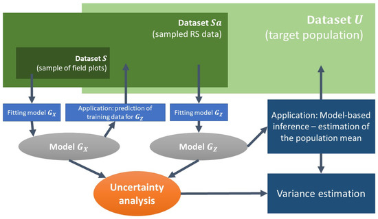
Figure 1.
Overview of Generalized Hierarchical Model-Based estimation.
We estimated by generalized least squares (GLS) estimators usinf dataset S e.g., [28]:
Conditions and in and , respectively, imply that for the superpopulation model , and for the superpopulation model , . This does not imply that equals for a given realization of and . For example, assume tree biomass is modeled based on either tree diameter () or tree height () these two models will be very different, and in formal terms this is because the models provide the expected values conditional on the different predictor variables. This difference between the two models may be more subtle when the models are based on different types of RS data, but the principle remains the same: the two models will be different. Thus, for a given realization of and , , but . Using the models (1) and (2) we obtain , and thus,
where is a random variable. It can be seen that ( and are vectors of average values) and thus, the relationship agrees with . The relationship (4) is employed to estimate the model parameters using the dataset and , i.e.,
The variance-covariance matrices and are among the essential parameters to be estimated. Under assumptions of homoskedasticity and independence, and become and .
However, under heteroskedasticity and dependent observations the form of and is different. Under heteroskedasticity, the matrices’ diagonal elements, corresponding to individual error variances, are unequal. Dependent errors may arise due to several reasons, important examples are clustered sample data, spatially autocorrelated errors and nested samples:
- with clustered data structure, and are block-diagonal matrices, where the blocks correspond to the clusters;
- under spatial autocorrelation, the matrices’ off-diagonal elements, corresponding to covariances between errors, are non-zero;
In the present study we didn’t account for the uncertainty due to the estimation of and , and assumed that they are known to a constant, i.e., and . This is a common practice when GLS estimators are applied cf. [28,29]. Therefore, since the and terms will cancel, estimators (3) and (5) can be rewritten as
and
The difference between (3) and (6), and (5) and (7) is that the covariance matrices are not estimated in (6) and(7) but assumed known cf. [28,29].
The expected value of the finite population mean is then estimated as
where the subscript GHMB denotes “Generalized Hierarchical Model-Based” and is an N-length vector, each element of which is .
The variance of is
where (see Appendix A for details) is the core expression for the GHMB estimator variance. As shown in the Appendix A the covariance composed of four terms.
where
In the general case all these terms would be non-zero and contribute to the variance of the GHMB estimator. However, in case the S and datasets are independent, then . By replacing and with the corresponding estimators and we obtain the covariance estimator , i.e.,
where in model (1) is estimated as e.g., [28]
whereas due to relationship (4), was estimated as
where , is an identity matrix of dimension and . The correction is needed because the response variable in relationship (4) is not measured but estimated using estimator (6).
It can be seen that the estimated covariance of is a part of by substituting in estimator (11) to e.g., [28]. The derivation of estimators (11) and (13) are presented in Appendix A. Our GHMB variance estimator is
2.3. Reference Methods for Comparison
We compared the performance of the GHMB estimator with the two-stage model-based estimation procedure presented in [18], which utilizes the same datasets. Additionally, we compared the GHMB estimator with estimators utilizing only a single source of RS data, i.e., an estimator for hybrid inference [24], and an estimator for conventional model-based inference e.g., [17]. Some details of these reference methods are provided below.
2.3.1. Generalized Two-Stage Model-Based Estimation (GTSMB)
In this estimation procedure, the regressors in the model , are regressands and dependent on , i.e.,
for the kth variable out of variables in . The same set of is used to predict each variable in . Model parameters are estimated using information from the dataset employing the GLS estimator, i.e., cf. [28]. Similarly to GHMB estimation, we do not account for the uncertainty due to the estimation, and, thus, assume to be known to a constant , i.e., . Thus,
In this approach the expected value of the finite population mean, , is estimated as
where and the subscript GTSMB denotes “Generalized Two-Stage Model-Based”. The variance of is estimated as
where = and .
Details of the estimator (18) are presented in [18]. The R package “HMB” by Saarela et al. [30] was used to obtain estimates based on (17) and (18).
The correspondence between GHMB and GTSMB estimators were further evaluated as a part of this study. In Appendix B we show that under certain rather general conditions the estimators and variance estimators will provide approximately the same results for given datasets.
2.3.2. Hybrid Estimation
We employed the hybrid estimators for clustered data described in [24]. The estimator utilizes sampled data from the dataset, and accounts for sampling uncertainty due to the sample and modelling uncertainty due to the model (1) (i.e., ) using the dataset S [24].
Within hybrid inference, the population mean estimator is [24] (Equation (11), p. 101)
where m is the number of clusters in , is the ith cluster total, and is the number of population elements in the ith cluster.
The corresponding variance estimator is [24] (Equation (15), p. 101).
where .
2.3.3. Conventional Model-Based Inference (MB)
This estimation procedure uses only one source of auxiliary information available wall-to-wall, in our case the Landsat 7 ETM+ data. The population mean estimator is e.g., [17] (Equation (3), p. 899).
where is a vector of estimated model parameters using the dataset S following superpopulation model in Equation (2). As in the previous approaches, in this case we also assume that the covariance is known to a constant , i.e., .
The model-based variance estimator is
where and cf. [28].
3. Material
For this study we simulated six populations mimicking forest conditions in study areas across the USA (Figure 2). For each site reference data were available from field measurements, Landsat 7 ETM+, and laser scanning using a method that mimics future measurements with the GEDI space LiDAR. In this section we first describe the datasets and, secondly, how these reference data were used for simulating AGB and RS data for each study site.
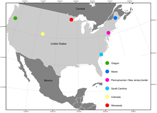
Figure 2.
Study sites across the USA.
3.1. Reference Data
3.1.1. Simulated GEDI Data
GEDI’s nominal footprint diameter will be approximately 25 m, with approximately 60-m along-track spacing [21]. After two years of operation aboard the International Space Station (ISS), the cross-track spacing of GEDI’s sample is expected to be 500 m, producing a semi-regular lattice of sample lines from 51 South to 51 North (the area of the Earth traversed by the ISS orbit). Waveform properties used in the modeling process were quantified by relative heights (rh) from below which different amounts of energy were reflected. So, ‘rh90’ was the height below which 90% of the waveform energy returned, which was higher by an amount dictated by the vertical distribution of canopy material than ‘rh30’.
The LiDAR data used in this study were derived by the GEDI Science Team from airborne discrete-return LiDAR (DRL) acquisitions, transformed to resemble the return waveforms to be collected by the GEDI mission. Further details related to LiDAR and field data acquisition are given in Appendix C. The transformation process is one where individual photon returns from across a given surface area are grouped into height quantiles, which are then integrated to derive a waveform describing the return height function for that area [32]. The GEDI Waveform Simulator realistically accounts for topographic and canopy penetration issues, while effecting the above physical transformation of return energy information from discrete to continuous functions.
The DRL acquisitions forming the basis of this study were collected with a RIEGL LMS-Q680i airborne laser scanner across the six study sites (Maine, Pennsylvania, South Carolina, Colorado, Minnesota) between June and August 2014, the Oregon site was scanned in June 2015. Data were collected in North-South lines that were 300–1000 m in width and spaced 5 km apart. Pulse density was at least 4 pulses per square meter. The DRL sample lines were transformed to simulate a surface of contiguous GEDI footprints along the sample lines. Ten strips of GEDI data, each about 510 m long, were available from each site [33].
3.1.2. Landsat 7 ETM+ Data
Landsat values were derived for each field plot from surface reflectance values (multiplied by 10) generated from the LEDAPS algorithm [34]. Pre-collection surface reflectance imagery from June to September 2015 for band 3 (red; B3) and band 4 (near-infrared; B4) were composited using a medoid method (multi-dimensional median; [35]), screening out clouds and cloud shadows using the F-mask algorithm [36]. This processing was conducted on the Google Earth Engine platform [37].
3.1.3. Field Data
Between 46 and 50 field plots were established in each of the six study sites from June–August, 2014 (Maine, Pennsylvania, South Carolina, Colorado, Minnesota) and from June–August 2015 (Oregon, see Appendix C for more details). The sample was designed to cover the range of vegetation conditions in each area, making use of 15 strata covering the bivariate distribution of LiDAR-based estimates of height (broken into 5 classes) and vegetation cover (3 classes). The sampled distribution excluded locations with less than 10% canopy cover (according to LiDAR metrics) and areas of non-forest according to the National Land Cover Dataset [38]. Approximately 25 random locations were chosen within each stratum, from which an approximately equal number (3–4) were chosen for field measurement based upon accessibility.
Standard field protocols used by the US National Forest Inventory (managed by the US Forest Service Forest Inventory and Analysis program) were used in measuring trees on 16.15 m radius plots (yielding approximately the same area plot as a Landsat pixel) [39]. For details see Appendix C. AGB was calculated from the tree list for each plot as described in [39]. Plot numbers, forest types according to [40,41] and statistics are summarized in Table 1.

Table 1.
Overview of field data.
3.2. Simulated Populations
Each of the six areas depicted in Figure 2 were simulated independently; each contained approximately 50 field plots, with corresponding Landsat 7 ETM+ and GEDI data (simulated from DRL). In general, the target for the GEDI mission is to report AGB estimates by 1-km squares. Thus, the setup will be according to Figure 3a, i.e., the area is tessellated into 1-km grid-cells, each of which will have a certain number of GEDI footprints (the points) and potentially a wall-to-wall cover of Landsat data.
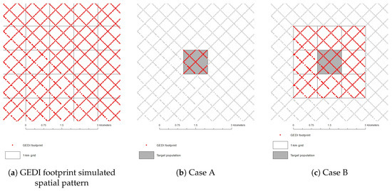
Figure 3.
(a) Simulated spatial pattern of GEDI footprints and the 1-km grid delineation; (b) Case A: data for a single 1-km grid-cell were used; (c) Case B: data from neighboring grid-cells were used as well, for the GHMB and GTSMB estimators.
Our case study examples are of two kinds. In Case A, only data (GEDI and Landsat 7 ETM+) from within a given 1-km grid-cell are used. In Case B, data from eight neighboring grid-cells were used in addition to the center (target) grid, since model development data from a larger similar area may improve GHMB estimation. Note, that only the GHMB and GTSMB approaches can benefit from data from surrounding grid-cells, since such data can be used to improve the model used in the final step of the GHMB (and GTSMB) procedure, that is, developing a model linking predicted biomass values (based on GEDI data) with wall-to-wall Landsat data, and in the case of GTSMB procedure developing a multivariate model linking GEDI variables with Landsat data. The conventional MB and the hybrid methods cannot benefit from including a support area of this kind. The two cases are shown in Figure 3b,c.
Simulation were made to provide the data needed for Case B; Case A data were obtained as the corresponding data from the center 1-km grid-cell. Each 1-km grid-cell was tessellated into 2500 square plots of a size corresponding to the future GEDI LiDAR footprint size.
Correlated Multinomial Random Variables
To create our simulated populations mimicking forest conditions in the study sites we need correlation matrices between the AGB, GEDI and Landsat 7 ETM+ variables. The matrices were calculated using reference data and are given in Table 2.
Table 2.
Correlations between the study variables for each study site.
We applied a classical method for generating correlated multivariate normal random variables for a given covariance matrix, i.e.,
where, is the desired multivariate normal vector of t variables (in our case study the variables are AGB, rh60, rh90, B3 and B4), is a row vector of independent standard normals, is the vector of corresponding means, and is a triangular matrix such that . We applied Cholesky decomposition to derive the matrix . The covariance matrix and the expected values were estimated using reference data for each study site. Table 3 provides and expected values for each study site.
Table 3.
Mean values and standard deviations of the study variables for each site.
The independent vector of standard normal random variables was generated randomly for a given simulated spatial autocorrelation of exponential form as a function of spatial distances between square plots, i.e., . The spatial autocorrelation values are presented in Table 4.
Table 4.
Simulated spatial autocorrelation between two square plots center-points at 20 m distance for AGB variable for each study site.
We emphasis that for purposes of this study we assumed AGB autocorrelation as an average of GEDI rh60 and rh90 autocorrelation values (estimated using GEDI simulated strip data), given strong correlation between AGB and GEDI variables. This is an important point that the AGB autocorrelation assessment was not a part of the computation process.
3.3. Regression Modeling
For each study site five regression models were fitted. Table 5 gives the model description and Table 6 provides information on the degrees of freedom, which were employed in the regression models involved for the different estimation methods. Dataset S was randomly selected from the square plots belonging to the target population U (1-km grid-cell) and its support area (eight neighboring 1-km grid-cells) corresponding to Case B, i.e., from the km area (see Figure 3c).
Table 5.
The regression models employed in the case study sites.
Table 6.
Degree of freedom (df) for the models involved.
3.4. Evaluation Criteria
We used the relative standard error (rSE) to assess the precision of the estimators
where is the expected value of population mean and in our study cases is the mean value of AGB over field plots (see Table 3).
We also analyzed the uncertainty contribution of different sources in GHMB and hybrid estimation, i.e., for GHMB uncertainty contribution (i) due to the AGB-GEDI model, and (ii) due to the AGB-Landsat (Sa) model; for hybrid uncertainty contribution (i) due to the modeling, and (ii) due to the sampling. We estimated proportions of each uncertainty contribution, i.e., for GHMB estimation the proportions are estimated as (estimator (11) with substituting to , and estimator (14)):
for hybrid estimation the proportions are estimated as (estimator (20)):
Ideally the performance of estimators and variance estimators should have been evaluated through Monte Carlo simulations with repeated simulation of both the populations and selection of datasets S and , and the estimations. However, as seen from the formulas (11) and (14) the variance estimator is conditional on the sample outcomes and . Thus different simulated samples will result in different variances. It is the random deviations and that causes uncertainty according to the formulas. Therefor simulations that result in different and cannot strictly be used to compare the empirical variance with the mean estimated. The simulated variances should be seen as examples of the size. For this reason we have chosen a restricted number of simulations. Simulations of only and could be used for empirical studies, but then (for a given set of simulations) only for a single fixed sample and .
4. Results
In Table 7, the expected population mean AGB values, , the corresponding simulated mean values, , and the estimates for the GHMB and GTSMB (Cases A and B), hybrid, and MB methods are presented. It can be seen that the AGB varied quite substantially between the different sites with the highest value in Oregon and the lowest in Minnesota. The average of estimated values over 250 repetitions were always fairly close to the average of simulated true means, .
Table 7.
Estimated expected value of population mean, , [Mg/ha].
Our assessment of the performance of the different methods is based on estimated variances, recalculated and expressed as relative standard errors, for each method in each of the study areas as well as on average across the different study areas.
In Figure 4, the average relative standard error for the different methods across the study sites is presented. In this case a relative variance was first estimated for each site; then an average for the sites was calculated from which the square root was computed. On average, the GHMB and GTSMB methods performed about equally well (Appendix B), and they were superior to the other methods in case data from neighboring grid cells were used for improving the models (case B). When data from the target grid cell, only, were used for the model building (case A), the GHMB and GTSMB methods were outperformed by the hybrid and conventional MB estimation methods.
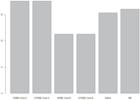
Figure 4.
The average relative standard error for the different methods, [%].
Relative standard error for each of the methods in each site is detailed in Table 8. It can be seen that the performance of the methods, in terms of relative standard error, varied substantially between the sites. The hybrid estimation method showed fairly consistent results, in terms of precision, across the different sites with the smallest relative standard error in Colorado and the largest in Pennsylvanian and New Jersey border. In this simulation study we were not able to indicate any specific relation between estimators’ performance and forest types. To conduct such analysis, real life data would be required rather than simulated. The MB method performed almost as well as hybrid estimation with similar patterns across study sites, and GHMB and GTSMB Case A estimations. The GHMB and GTSMB methods typically decreased their relative standard errors by about 40% when data from surrounding grid-cells were applied in the model building.
Table 8.
Relative standard error in the study sites, , [%].
Sources of Uncertainty for the GHMB and Hybrid Estimation Methods
Table 9 shows the contribution of different sources of uncertainty to the variance GHMB and hybrid estimation methods. It can be seen that the contribution of the AGB-GEDI estimated model uncertainty is substantial for both estimation methods; for GHMB Case A it varies between 19% (MN) and 47% (CO), in Case B between 54% (CO) and 81% (MN), and in hybrid estimation between 24% (ME) and 60% (PANJ). Comparing Cases A and B in GHMB estimation, we can see that with an increased number of GEDI footprints (from 94 to 727), the uncertainty contribution of the AGB-Landsat (Sa) estimated model decreased.
Table 9.
Proportion (percentage) of the variance due to different sources for the GHMB and hybrid estimation methods, [%].
5. Discussion
In this article the hierarchical model-based estimation method presented by Saarela et al. [17] has been extended to cases when the model errors have non-homogeneous variance and cases where the errors are correlated, for example due to clustered sample data and/or spatial autocorrelation. A main component of this development is that generalized least squares theory is applied for the parameter estimation in the regression analysis, in which case the parameter estimation and the corresponding estimation of the covariance matrix for the parameter estimates accommodate such data structures. Also, the similarities between the GHMB and the GTSMB methods [18] are further explored and a proof is given (Appendix B) that the two methods will provide identical estimates and variances, and almost identical variance estimates, under certain conditions. However, with the expansion of the GHMB theory presented in this article, the GHMB method has a potential to be applied under a wider range of conditions than the GTSMB method, which among other things assumes independence between the two datasets used for the model building. The GHMB method might also be considered more intuitive to apply since it directly predicts the reference data (AGB values) that are used for the model building in the final step. The GTSMB method, on the other hand, uses the wall-to-wall RS data for predicting the metrics that would have been obtained from the sampled RS data source.
The results from the case studies indicate that the GHMB and GTSMB methods lead to more precise results, when a large support area is used for developing the model linking the wall-to-wall dataset (simulated Landsat data in our case) with the model predictions from the sample RS data (simulated GEDI data in our case). Restricting the data for the model building to a smaller area decreases the precision of the two methods. The hybrid estimation method and the conventional MB method were superior to the GHMB and GTSMB methods when only a 1-km support area was used. With the hybrid method, the AGB predictions from the GEDI sample, only, are used for the inference in our case. The conventional MB method makes predictions for all units in the wall-to-wall dataset (simulated Landsat data). Note, that Case B is only relevant for GHMB and GTSMB, since the dataset S (the field sample plots) was assumed to have a fixed size regardless of the size of the target area, and thus, the models used for the MB estimation would be the same in Case A and Case B. Thus “borrowing strength” for the model development from surrounding grid-cells does not change anything in the cases of conventional MB estimation. This holds true also for hybrid estimation, based on the same argument.
Overall, the performance of the different methods depends on many factors. A first requirement is that the study area is large enough, so that the assumption that the superpopulation mean value is approximately the same as the study area mean holds. Further, the goodness-of-fit of the models involved is another core issue. With a very good model linking wall-to-wall data with AGB values, there is no need for complicating the estimation with hybrid, GHMB or GTSMB methods. However, most wall-to-wall RS datasets are weakly correlated with AGB which is the reason why samples of RS data that are strongly correlated with AGB are of interest as additional sources of auxiliary data in more advanced estimation procedures. Lastly, the sample sizes of the S and datasets are important for the precision of the estimators. In general, increasing the sample sizes will increase their precision. Table 9 supports this statement, as it shows that 47 degree of freedom for fitting the AGB-GEDI model resulted in low precision of estimated and, hence, the uncertainty contribution to the estimated variance in GHMB estimation for Case A was between 38% and 19%, and for Case B between 62% and 87%. The low precision of estimated lead to the situation that the conventional MB method with only one source of weakly correlated wall-to-wall RS data (simulated Landsat data in our example) slightly outperformed GHMB (and GTSMB) in Case A, where only 94 GEDI footprints were available (see Figure 4).
The niche for GHMB and GTSMB estimation appears to be the important cases where the following requirements are fulfilled: (i) field data are sparse and expensive to acquire, (ii) wall-to-wall RS data (or a large sample of RS data) are available, which can be fairly well fit to the target variable, and (iii) RS data which can be very well fit to the target variable are available, but only samples of such data can be acquired. Since AGB models based on laser data can be expected to be more generally applicable across large regions than AGB models from Landsat data, it should make sense to train local models of the latter kind using pseudo-field data from predictions with the former kind of models, and thus apply GHMB or GTSMB estimation.
Several methodological issues may be brought up in relation to this study:
- One important issue is that all the case study data were simulated, based on sparse samples of reference data. The simulations are simplified generalizations of the real world, that leave out many important issues that must be handled in practical surveys, such as delineating forests from non-forest land [42]. In practical applications, land-use maps need to be applied to delineate forests before the GHMB method is employed.
- Another important restriction of the present study is that the results are based on estimates from a small number of iterations. A future expanded study should be based on Monte Carlo simulations of both the populations and the sampling from these populations, as a basis for empirical evaluation of the proposed estimators. Another method for simulating the multivariate variable in Equation (23) might be applied to demonstrate explicitly abilities of the proposed estimators.
- Further, future studies on this subject should also deal with the details of how to estimate the correlation matrices of model errors that are required for the GLS regression; in this article these details are only briefly addressed. One of the solutions to this problem could be iterative re-weighted least squares regression methods, such methods are often applied in geostatistical approaches.
- The current GHMB estimator is derived under the assumption that the target population is large, i.e., so that the population mean is at least approximately equal to the superpopulation mean. Modifications of the GHMB estimators for small-area estimation should be addressed in a potential future study.
- In the current study we assumed that the regression models involved in the AGB assessment by means of GEDI and Landsat data are linear. However, in reality the relationship between AGB (or growing stock volume) and height-like measures tends to be nonlinear e.g., [23]. A further elaboration of the GHMB method for nonlinear models would be needed to handle such cases.
- Lastly, the performance of GHMB method in comparison to other methods should be analyzed as a basis for making recommendations on what method is appropriate under different conditions.
The above issues identify areas of needed research in the context of our findings. Including those issues into the current study would have increased the scope and length of the article considerably, and, thus, we chose to put those issues on hold for future studies.
6. Conclusions
Design-based inventory methods based on field sampling are limited by the availability of plot data. GHMB (and GTSMB) allows estimation of biomass in areas where there may be none or very limited field data, such as the 1-km grid-cells of interest to the GEDI mission, by taking advantage of multiple levels of RS data. Specifically, field data and high-quality RS data from similar areas outside the domain of interest can be used to calibrate wall-to-wall predictions within the domain of interest using synoptically collected RS data more weakly related to biomass. This paper augments previous hierarchical estimation methods by presenting methods that can be applied in cases where model errors have non-homogenous variance and where the model errors are correlated. Both cases are relevant for use of data from the upcoming GEDI LiDAR mission.
Author Contributions
Conceptualization, S.S., S.H. and G.S.; Data curation, S.S., S.P.H., H.-E.A. and P.L.P.; Funding acquisition, S.P.H. and E.N.; Investigation, S.S., S.H., S.P.H., H.-E.A., H.P., W.P., P.L.P., E.N., T.G.G. and G.S.; Methodology, S.S., S.H. and G.S.; Project administration, S.S., S.P.H. and E.N.; Software, S.S. and S.H.; Writing—original draft, S.S., S.H. and G.S.; Writing—review & editing, S.S., S.H., S.P.H., H.-E.A., H.P., W.P., P.L.P., E.N., T.G.G. and G.S.
Funding
Funding was provided by grants from NASA’s Carbon Monitoring System (Healey CMS2016, Cohen CMS2013) and ERA-GAS FORCLIMIT (grant number FR-2017/0006).
Acknowledgments
The authors gratefully acknowledge Steven Hancock of the University of Maryland, who simulated the GEDI waveforms, Warren Cohen (US Forest Service), who helped to direct much of the field and LiDAR data collection, Zhiqiang Yang (US Forest Service), who helped in the development of “HMB” R package, and GEDI Science Team. The authors are thankful to the four anonymous Reviewers, whose comments helped to improve the clarity of the article.
Conflicts of Interest
The authors declare no conflict of interest.
Abbreviations
| AGB | AboveGround Biomass |
| GEDI | Global Ecosystem Dynamics Investigation |
| GHMB | Generalized Hierarchical Model-Based |
| GLS | Generalized Lest Squares |
| GTSMB | Generalized Two-Stage Model-Based |
| Landsat 7 ETM+ | Landsat 7 Enhanced Thematic Mapper Plus |
| LiDAR | Light Detection And Ranging |
| MB | Model-Based |
| NFI | National Forest Inventory |
| PALS | Portable Airborne Laser System |
| RS | Remote Sensing |
| UNFCCC | United Nations’ Framework Convention on Climate Change |
Appendix A. Generalized Hierarchical Model-Based Estimators
For a realization, i.e., our target population, we have superpopulation models:
We also defined the following relationship between the two models for the given realization:
For given datasets S, Sa, and U, and matrices and :
Knowing that and , we have
Due to :
Due to :
Denoting , and given that , we have
This gives
Thus, covariance is
where
Under the assumption, :
Knowing that e.g., [28] we can rewrite
Here we show that the trivial estimator for through the sum of squared residuals divided by the degree of freedom, leads to a biased estimation. We also derive an unbiased estimator.
We denote . The expected value of is:
Denoting and we have
Due to (for the given realization of and ):
Therefore,
Given we have
And thus, the expected value of the sum of squared residuals is (note: here we used that the quadratic form for any column vector and matrix ),
Knowing that , and , we have
Given and we have
Thus,
It can be seen that estimator is biased, and thus, to derive an unbiased estimator we have to correct for the estimated BIAS, i.e.,
And thus,
Under the independence assumption between datasets S and , , we have
Knowing that we can rewrite estimator as
Appendix B. A Comparison between Expectations and Variance Estimators of the Two Methods: GHMB and GTSMB
Below it is shown that the two methods GHMB and GTSMB lead to identical results under certain conditions. Throughout below we neglect the effects of estimating covariance matrices and use notations as if the matrices were known to a constant.
We start with the estimators: for GHMB we have,
where, according to estimator (7)
For GTSMB we have the same . The link between GEDI and Landsat data is given by
The parameters are estimated from the sample and we have the GLS estimators
where should be understood as . From (A17) we obtain the vector of estimated GEDI values, given the Landsat ones as the columns of , where is the matrix with the vectors as columns.
Thus, for GTSMB estimation we have the estimator
Comparing (A14) and (A18), we can see that , if
and thus
This is so because the cancel in (A17), and (A20) multiplied by is equal to .
The relation (A19) seems very restrictive. It means that the correlation matrices for the k error terms vectors are identical. However, this is not unrealistic as the GEDI variables are strongly correlated. Also, this common correlation matrix is assumed to be equal to the correlation matrix of the error terms of the GHMB model. This is not unrealistic either, since the GEDI variables should show a high correlation with field data y and so should the GHMB predictions . At least, the assumption (A19) is an acceptable approximation. In the homoskedastic GEDI-Landsat case (when and the are normed unit matrices) the relation (A19) holds automatically, whether the Field-GEDI relation is homoskedastic or not.
Thus, under certain conditions, exactly or approximately. Hence, the variances are so too. Still, it remains to see whether or not the two variance estimators are (almost) identical under some conditions. We restrict this study to the case where the S and samples are selected independently. The GHMB variance estimator is then (estimators (11) and (14))
where
The GTSMB variance estimator is (estimator (18))
We introduce the matrix that is the same for all k and that, in accordance with the condition (A19) is assumed to fulfill
for some constants , ( throughout). Then since cancels (see (A17)), and
Thus, the first term in the (A23) equals
Due to the assumptions (A19) and (A24) we also have for some constant . Since cancels in the second term of estimator (A22), we see that the contribution of this term to equals the first term in .
Next, we will show that he first term of equals to the second one in . For this we need to add that condition (A24) also holds for the cross-covariances, i.e., that
We have, since cancels,
and from this and (A27) we obtain
Hence, by summation, we obtain for the second term of
Next we will show that (where ), exactly or approximately, and then
In the hierarchical approach for the given realization of and we have
We insert the second stage model (A16) of the two-stage approach,
to get
We identify the fixed and random parts of expression (A33) and see that
Written in a clear way, we have (omitting the index )
By taking the expectation of the product of the two sides of (A35) with their transposes we obtain
Recalling that and , we have
and, thus, by replacing expected values with their estimators,
what is exactly the first term of the .
Numerical examples (with simulated data) have shown that the two first terms of the variances give identical sums. Further, the size of the third term of has been shown to be much smaller that the other two (it contributed with about 0.5% of the variance). The third term could be seen as a second order correction of the first two.
Appendix C. Field and LiDAR Data Collection Methods
LiDAR data were collected using a Riegl LMS-Q680i system at five sites (SC, PANJ, ME, MN, CO) in the summer of 2014 and a sixth site (OR) in the summer of 2015 (see Figure 2 for locations and Table 1 for site descriptions). All data were collected during snow-free time periods when vegetation was fully leaf-on and non-senescent. The data was collected in north-south oriented flight lines spaced 5 km apart. Some crossing flights were flown for calibration purposes. Technical specifications for the LiDAR acquisition included: point density of 4 pulses per square meter; altitude of 732 m; field of view of 60 degrees; pulse rate of 330 kHz; nominal swath width of 812 m; horizontal and vertical accuracy (root mean square error in z) of 50 cm [33]. The LiDAR data were processed in Fusion [43] to produce rasters of various metrics with a 30 m cell size to support the plot selection process described below.
Approximately fifty field inventory plots were established at each area in the summer of 2015 [44]. To ensure that field plots represented the full range of biomass levels within forested areas of each scene, the LiDAR data was used to inform the selection of field plot locations via a stratified sampling procedure. After masking out non-forest areas within the LiDAR coverage using a LiDAR-based percent cover threshold (10%) and the National Land Cover Dataset [38], fifteen strata were delineated based upon three vegetation cover and five height classes within the random cells. A minimum of 23–24 candidate plot locations were generated for each of the 15 identified strata. Final field plots were selected from these candidate plots on the basis of accessibility and valid forest land cover status. Once in the field, crews aimed to visit 50 sample plots at each study area, with 3–4 plots in each stratum.
At each plot location, live and dead trees with dbh > 12.7 cm were measured on a 16.2-m radius plot, and trees with 2.54 cm < dbh < 12.7 cm were measured on a 4.57-m radius circular plot. Field protocols consistent with those used by the US Forest Service were used in measuring trees [39]. In addition, survey-grade GPS coordinates (<1 m error) were acquired for each plot center.
Large-footprint LiDAR waveforms similar to those expected from GEDI were simulated from the acquired lidar data using the method presented in [32], in which waveforms are modeled as the sum of individual returns from surfaces at different heights, accounting for instrument-specific properties. Realistic noise was added to the simulated waveforms following [45,46]. The expected signal to noise ratio (SNR) of GEDI signals has been predicted through link margin analysis. For a given SNR, the probability of the ground elevation being correctly identified can be calculated and used to quantify the expected measurement accuracy. The simulator has been validated against real LVIS data (airborne large-footprint, full-waveform liDAR similar to GEDI; [47]) in terms of waveform metrics and metric accuracy in the presence of noise.
References
- UNFCCC. United Nations Framework Convention on Climate Change. Available online: http://unfccc.int/resource/convkp/kpeng.html (accessed on 5 September 2017).
- Europe, F.; Unece, F. State of Europe’s Forests 2011. Available online: https://library.wmo.int/index.php?lvl=notice_display&id=5268#.W_PPmcTNWUm (accessed on 5 September 2017).
- Wulder, M.A.; White, J.C.; Nelson, R.F.; Næsset, E.; Ørka, H.O.; Coops, N.C.; Hilker, T.; Bater, C.W.; Gobakken, T. Lidar sampling for large-area forest characterization: A review. Remote Sens. Environ. 2012, 121, 196–209. [Google Scholar] [CrossRef]
- McRoberts, R.E.; Wendt, D.G.; Nelson, M.D.; Hansen, M.H. Using a land cover classification based on satellite imagery to improve the precision of forest inventory area estimates. Remote Sens. Environ. 2002, 81, 36–44. [Google Scholar] [CrossRef]
- Saarela, S.; Grafström, A.; Ståhl, G.; Kangas, A.; Holopainen, M.; Tuominen, S.; Nordkvist, K.; Hyyppä, J. Model-assisted estimation of growing stock volume using different combinations of LiDAR and Landsat data as auxiliary information. Remote Sens. Environ. 2015, 158, 431–440. [Google Scholar] [CrossRef]
- Grafström, A.; Schnell, S.; Saarela, S.; Hubbell, S.; Condit, R. The continuous population approach to forest inventories and use of information in the design. Environmetrics 2017, 28. [Google Scholar] [CrossRef]
- Matérn, B. Spatial Variation: Stochastic models and their applictation to some problems in forest surveys and other sampling investiagtions. Meddelanden från Statens Skogsforskningsinstitut 1960, 49, 144. [Google Scholar]
- Gregoire, T.G. Design-based and model-based inference in survey sampling: Appreciating the difference. Can. J. For. Res. 1998, 28, 1429–1447. [Google Scholar] [CrossRef]
- McRoberts, R.E.; Magnussen, S.; Tomppo, E.O.; Chirici, G. Parametric, bootstrap, and jackknife variance estimators for the k-Nearest Neighbors technique with illustrations using forest inventory and satellite image data. Remote Sens. Environ. 2011, 115, 3165–3174. [Google Scholar] [CrossRef]
- Särndal, C.E.; Swensson, B.; Wretman, J.H. Model Assisted Survey Sampling; Springer: New York, NY, USA, 1992; p. 716. [Google Scholar]
- Gregoire, T.G.; Ståhl, G.; Næsset, E.; Gobakken, T.; Nelson, R.; Holm, S. Model-assisted estimation of biomass in a LiDAR sample survey in Hedmark County, Norway. Can. J. For. Res. 2011, 41, 83–95. [Google Scholar] [CrossRef]
- Massey, A.; Mandallaz, D.; Lanz, A. Integrating remote sensing and past inventory data under the new annual design of the Swiss National Forest Inventory using three-phase design-based regression estimation. Can. J. For. Res. 2014, 44, 1177–1186. [Google Scholar] [CrossRef]
- Chirici, G.; McRoberts, R.E.; Fattorini, L.; Mura, M.; Marchetti, M. Comparing echo-based and canopy height model-based metrics for enhancing estimation of forest aboveground biomass in a model-assisted framework. Remote Sens. Environ. 2016, 174, 1–9. [Google Scholar] [CrossRef]
- Boudreau, J.; Nelson, R.F.; Margolis, H.A.; Beaudoin, A.; Guindon, L.; Kimes, D.S. Regional aboveground forest biomass using airborne and spaceborne LiDAR in Québec. Remote Sens. Environ. 2008, 112, 3876–3890. [Google Scholar] [CrossRef]
- Nelson, R.; Boudreau, J.; Gregoire, T.G.; Margolis, H.; Næsset, E.; Gobakken, T.; Ståhl, G. Estimating Quebec provincial forest resources using ICESat/GLAS. Can. J. For. Res. 2009, 39, 862–881. [Google Scholar] [CrossRef]
- Neigh, C.S.; Nelson, R.F.; Ranson, K.J.; Margolis, H.A.; Montesano, P.M.; Sun, G.; Kharuk, V.; Næsset, E.; Wulder, M.A.; Andersen, H.E. Taking stock of circumboreal forest carbon with ground measurements, airborne and spaceborne LiDAR. Remote Sens. Environ. 2013, 137, 274–287. [Google Scholar] [CrossRef]
- Saarela, S.; Holm, S.; Grafström, A.; Schnell, S.; Næsset, E.; Gregoire, T.G.; Nelson, R.F.; Ståhl, G. Hierarchical model-based inference for forest inventory utilizing three sources of information. Ann. For. Sci. 2016, 73, 895–910. [Google Scholar] [CrossRef]
- Holm, S.; Nelson, R.; Ståhl, G. Hybrid three-phase estimators for large-area forest inventory using ground plots, airborne lidar, and space lidar. Remote Sens. Environ. 2017, 197, 85–97. [Google Scholar] [CrossRef]
- Gobakken, T.; Næsset, E.; Nelson, R.; Bollandsås, O.M.; Gregoire, T.G.; Ståhl, G.; Holm, S.; Ørka, H.O.; Astrup, R. Estimating biomass in Hedmark County, Norway using national forest inventory field plots and airborne laser scanning. Remote Sens. Environ. 2012, 123, 443–456. [Google Scholar] [CrossRef]
- Puliti, S.; Saarela, S.; Gobakken, T.; Ståhl, G.; Næsset, E. Combining UAV and Sentinel-2 auxiliary data for forest growing stock volume estimation through hierarchical model-based inference. Remote Sens. Environ. 2018, 204, 485–497. [Google Scholar] [CrossRef]
- Dubayah, R.; Goetz, S.; Blair, J.B.; Fatoyinbo, T.; Hansen, M.; Healey, S.P.; Hofton, M.; Hurtt, G.; Kellner, J.; Luthcke, S.; et al. The Global Ecosystem Dynamics Investigation. Available online: http://adsabs.harvard.edu/abs/2014AGUFM.U14A.07D (accessed on 3 July 2018).
- Tomppo, E.; Gschwantner, T.; Lawrence, M.; McRoberts, R.; Gabler, K.; Schadauer, K.; Vidal, C.; Lanz, A.; Ståhl, G.; Cienciala, E.; et al. National Forest Inventories. Pathways for Common Reporting; Springer: Berlin/Heidelberg, Germany, 2010; p. 614. [Google Scholar]
- Saarela, S.; Schnell, S.; Grafström, A.; Tuominen, S.; Nordkvist, K.; Hyyppä, J.; Kangas, A.; Ståhl, G. Effects of sample size and model form on the accuracy of model-based estimators of growing stock volume. Can. J. For. Res. 2015, 45, 1524–1534. [Google Scholar] [CrossRef]
- Ståhl, G.; Holm, S.; Gregoire, T.G.; Gobakken, T.; Næsset, E.; Nelson, R. Model-based inference for biomass estimation in a LiDAR sample survey in Hedmark County, Norway. Can. J. For. Res. 2011, 41, 96–107. [Google Scholar] [CrossRef]
- McRoberts, R.E. A model-based approach to estimating forest area. Remote Sens. Environ. 2006, 103, 56–66. [Google Scholar] [CrossRef]
- Cassel, C.M.; Särndal, C.E.; Wretman, J.H. Foundations of Inference in Survey Sampling; Wiley: Hoboken, NJ, USA, 1977; p. 192. [Google Scholar]
- Ståhl, G.; Saarela, S.; Schnell, S.; Holm, S.; Breidenbach, J.; Healey, S.P.; Patterson, P.L.; Magnussen, S.; Næsset, E.; McRoberts, R.E.; et al. Use of models for improved estimation in sample-based large-area forest surveys: A review. For. Ecosyst. 2016, 3, 1–11. [Google Scholar] [CrossRef]
- Davidson, R.; MacKinnon, J.G. Estimation and Inference in Econometrics; Oxford University Press: Oxford, UK, 1993; p. 896. [Google Scholar]
- Melville, G.; Welsh, A.; Stone, C. Improving the efficiency and precision of tree counts in pine plantations using airborne LiDAR data and flexible-radius plots: Model-based and design-based approaches. J. Agric. Biol. Environ. Stat. 2015, 20, 229–257. [Google Scholar] [CrossRef]
- Saarela, S.; Holm, S.; Yang, Z. HMB: Hierarchical Model-Based Estimation Approach. R package version 1.0. 2018. [Google Scholar]
- Sanderson, C.; Curtin, R. Armadillo: A template-based C++ library for linear algebra. J. Open Source Softw. 2016, 1, 1–26. [Google Scholar] [CrossRef]
- Blair, J.B.; Hofton, M.A. Modeling laser altimeter return waveforms over complex vegetation using high-resolution elevation data. Geophys. Res. Lett. 1999, 26, 2509–2512. [Google Scholar] [CrossRef]
- Andersen, H.E.; Cohen, W.B.; Yang, Z.; Healey, S.P.; Patterson, P.L.; Dubayah, R. Model-assisted estimation of carbon using Landsat and a designed sample of lidar data. Environ. Res. Lett. 2018, in press. [Google Scholar]
- Masek, J.G.; Vermote, E.F.; Saleous, N.E.; Wolfe, R.; Hall, F.G.; Huemmrich, K.F.; Gao, F.; Kutler, J.; Lim, T.K. A Landsat surface reflectance dataset for North America, 1990–2000. IEEE Geosci. Remote Sens. Lett. 2006, 3, 68–72. [Google Scholar] [CrossRef]
- Flood, N. Seasonal composite Landsat TM/ETM+ images using the medoid (a multi-dimensional median). Remote Sens. 2013, 5, 6481–6500. [Google Scholar] [CrossRef]
- Zhu, Z.; Wang, S.; Woodcock, C.E. Improvement and expansion of the Fmask algorithm: Cloud, cloud shadow, and snow detection for Landsats 4–7, 8, and Sentinel 2 images. Remote Sens. Environ. 2015, 159, 269–277. [Google Scholar] [CrossRef]
- Gorelick, N.; Hancher, M.; Dixon, M.; Ilyushchenko, S.; Thau, D.; Moore, R. Google Earth Engine: Planetary-scale geospatial analysis for everyone. Remote Sens. Environ. 2017, 202, 18–27. [Google Scholar] [CrossRef]
- Homer, C.; Dewitz, J.; Yang, L.; Jin, S.; Danielson, P.; Xian, G.; Coulston, J.; Herold, N.; Wickham, J.; Megown, K. Completion of the 2011 National Land Cover Database for the conterminous United States—Representing a decade of land cover change information. Photogramm. Eng. Remote Sens. 2015, 81, 345–354. [Google Scholar]
- CMS. Carbon Monitoring System (CMS) Field Guide 2015. In Pacific Northwest Research Station, USDA Forest Service; CMS: Portland, OR, USA, 2015; p. 82. [Google Scholar]
- Ruefenacht, B.; Finco, M.; Nelson, M.; Czaplewski, R.; Helmer, E.; Blackard, J.; Holden, G.; Lister, A.; Salajanu, D.; Weyermann, D.; et al. Conterminous US and Alaska forest type mapping using forest inventory and analysis data. Photogramm. Eng. Remote Sens. 2008, 74, 1379–1388. [Google Scholar] [CrossRef]
- Cohen, W.B.; Healey, S.P.; Yang, Z.; Stehman, S.V.; Brewer, C.K.; Brooks, E.B.; Gorelick, N.; Huang, C.; Hughes, M.J.; Kennedy, R.E.; et al. How similar are forest disturbance maps derived from different Landsat time series algorithms? Forests 2017, 8, 98. [Google Scholar] [CrossRef]
- McRoberts, R.E. Probability- and model-based approaches to inference for proportion forest using satellite imagery as ancillary data. Remote Sens. Environ. 2010, 114, 1017–1025. [Google Scholar] [CrossRef]
- McGaughey, R. FUSION/LDV: Software for LIDAR Data Analysis and Visualization, Version 3.01. Available online: http://forsys.cfr.washington.edu/fusion/fusionlatest.html (accessed on 24 August 2012).
- Legner, K.; Andersen, H.E.; Dobelbower, K.; Cooke, A.; Cohen, W.; Healey, S.P. A cost-effective field measurement protocol to support carbon monitoring—Implementing a prototype design at six different US sites (SC, NJ/PA, ME, MN, CO, OR). Gen. Tech. Rep. 2018, in press. [Google Scholar]
- Davidson, F.M.; Sun, X. Gaussian approximation versus nearly exact performance analysis of optical communication systems with PPM signaling and APD receivers. IEEE Trans. Commun. 1988, 36, 1185–1192. [Google Scholar] [CrossRef]
- Hancock, S.; Disney, M.; Muller, J.P.; Lewis, P.; Foster, M. A threshold insensitive method for locating the forest canopy top with waveform lidar. Remote Sens. Environ. 2011, 115, 3286–3297. [Google Scholar] [CrossRef]
- Blair, J.B.; Rabine, D.L.; Hofton, M.A. The Laser Vegetation Imaging Sensor: A medium-altitude, digitisation-only, airborne laser altimeter for mapping vegetation and topography. ISPRS J. Photogramm. Remote Sens. 1999, 54, 115–122. [Google Scholar] [CrossRef]
© 2018 by the authors. Licensee MDPI, Basel, Switzerland. This article is an open access article distributed under the terms and conditions of the Creative Commons Attribution (CC BY) license (http://creativecommons.org/licenses/by/4.0/).