Tree Species Classification with Multi-Temporal Sentinel-2 Data


1
Department of Forestry and Wood Technology, Linnaeus University, 351 95 Växjö, Sweden
2
Department of Forest Resource Management, Swedish University of Agricultural Sciences, 90183 Umeå, Sweden
3
Department of Earth Sciences, University of Gothenburg, 405 30 Gothenburg, Sweden
*
Author to whom correspondence should be addressed.
Remote Sens. 2018, 10(11), 1794; https://doi.org/10.3390/rs10111794
Submission received: 28 August 2018
/
Revised: 6 November 2018
/
Accepted: 7 November 2018
/
Published: 12 November 2018
(This article belongs to the Special Issue Multitemporal Remote Sensing for Forestry)
Abstract
:The Sentinel-2 program provides the opportunity to monitor terrestrial ecosystems with a high temporal and spectral resolution. In this study, a multi-temporal Sentinel-2 data set was used to classify common tree species over a mature forest in central Sweden. The tree species to be classified were Norway spruce (Picea abies), Scots pine (Pinus silvestris), Hybrid larch (Larix × marschlinsii), Birch (Betula sp.) and Pedunculate oak (Quercus robur). Four Sentinel-2 images from spring (7 April and 27 May), summer (9 July) and fall (19 October) of 2017 were used along with the Random Forest (RF) classifier. A variable selection approach was implemented to find fewer and uncorrelated bands resulting in the best model for tree species identification. The final model resulting in the highest overall accuracy (88.2%) came from using all bands from the four image dates. The single image that gave the most accurate classification result (80.5%) was the late spring image (27 May); the 27 May image was always included in subsequent image combinations that gave the highest overall accuracy. The five tree species were classified with a user’s accuracy ranging from 70.9% to 95.6%. Thirteen of the 40 bands were selected in a variable selection procedure and resulted in a model with only slightly lower accuracy (86.3%) than that using all bands. Among the highest ranked bands were the red edge bands 2 and 3 as well as the narrow NIR (near-infrared) band 8a, all from the 27 May image, and SWIR (short-wave infrared) bands from all four image dates. This study shows that the red-edge bands and SWIR bands from Sentinel-2 are of importance, and confirms that spring and/or fall images capturing phenological differences between the species are most useful to tree species classification.
1. Introduction
Information about tree species distribution in the forest landscape is valuable for implementing sustainable forest management. Forest companies use tree species information for operational and tactical resource planning. Higher target achievement may be reached by having tree species information prior to silvicultural treatments. Furthermore, tree species composition is an indicator of biodiversity which is a vital part in forest certification schemes, such as the Forest Stewardship Council [1]. Current satellite systems, such as Sentinel-2, may facilitate production of tree species maps from local to national level.
The Sentinel satellite program is a part of Copernicus led by the European Union’s Earth Observation program, formerly known as Global Monitoring for Environment and Security (GMES), and aims to bring continuity to other medium resolution satellite-programs, such as Landsat and the Satellite Pour l’Observation de la Terre (SPOT; [2]). The Sentinel-2 system has a sun-synchronous polar orbit at an altitude of 786 km. The Multi-Spectral Instrument (MSI) is a passive, optical push-broom sensor that enables a 290 km swath width, which is the largest as compared to other multi-spectral, medium spatial resolution optical missions, such as Landsat and SPOT. A large swath width results in a shortened revisit time for Sentinel-2 (e.g., five days at the equator and about three days closer to the poles), increasing the possibility to get cloud-free images. The MSI is equipped with 13 bands of which three are in the red edge spectrum and two in the shortwave infrared spectrum [2].
In the visible spectrum (VIS, approximately 400–700 nm) leaves are mainly absorbing light due to the presence of foliar photosynthetic chlorophyll a and b and carotenoids [3,4]. Leaf morphology affects how photons are scattering within the mesophyll and results in high reflectance in the near-infrared spectrum (NIR, approximately 700–1400 nm) [5]. Water is driving the chemical absorption at 970 nm and 1200 nm and results in a drop in reflectance in these wavelengths [6]. Leaves contain cellulose-, nitrogen- and lignin molecules that reflect strongly in the short-wave infrared spectrum (SWIR, approximately 1400–3000 nm), but the spectral absorption of water overshadows this in vital leaves; cellulose-, nitrogen- and lignin molecules in dry leaves reflect more since water is absent [6]. Flowering, leaf-onset and senescence change the biophysical and structural properties, which is used to differentiate between tree species in multi-temporal satellite datasets [7].
Two recent studies using Sentinel-2 imagery have shown that the red-edge bands and the SWIR-bands are useful for discriminating between tree species [8,9]. Nelson [8] used multi-temporal Sentinel-2 imagery (2 May, 21 July and 28 August, all from 2016) and the Random Forest (RF) classifier to classify tree species groups in central Sweden. The information classes were Norway spruce (Picea abies), Scots pine (Pinus silvestris), mixed coniferous forest, mixed coniferous/deciduous forest, deciduous forest, deciduous hardwood forest, and deciduous forest with hardwoods. The results improved in general by using a multi-temporal approach, with the best overall accuracy resulting from the combination of the spring and summer images (~85.2%), hence excluding the early senescence image (from 28 August 2016). The lowest overall accuracy was obtained using only the image from August 28 (~74.8%). The best, uncorrelated band-combination was the red (B4), red edge 2 (B6), red edge 3 (B7) and SWIR-2 (B12) bands from the three dates. In a study by Immitzer et al. [9], P. abies, P. silvestris, European Larch (Larix decidua), Silver Fir (Abies alba), Common Beech (Fagus sylvatica), Oak (Quercus sp.) and a mixed class of broadleaves were classified in eastern Bavaria, Germany. Random Forest was used with a single fall image (13 August 2015). An overall accuracy of 66.2% was achieved and the red-edge band 1 (B5), SWIR 1 (B11) and the blue band (B2) were ranked as important variables. The low accuracy was explained by the image being taken too early in the fall to display spectral variation from senescence, having too few sample plots, and heterogeneous species distribution of the field plots.
Previous to Sentinel-2 data, tree species classification with multi-temporal medium resolution optical sensors such as Landsat was tried, based on the same concept of seasonal variation due to phenology (e.g., [10,11,12,13,14,15,16]). Wolter et al. [12] emphasized that classifying tree species with optical imagery is a hard task since the spectral variance is often greater within information classes than between them. Schriever et al. [13] and Mickelson et al. [10] noted that satellite images from the start and the end of the growing season are important since spring and fall are when the phenological variation between tree species is the highest. Zhu et al. [14] classified pine, oak and a mixed mesophytic class using a multi-seasonal Landsat dataset and Support Vector Machines, finding that use of all dates (March, April, May, July, September, October and November) gave the highest Kappa accuracy (84%) as compared to fewer image date combinations (e.g., 72% for four images). Using Recursive Feature Elimination, however, they identified eleven bands of higher significance, which were primarily green, red, NIR and SWIR bands from one or two of the spring and fall images.
Prior studies with other data sources (e.g., hyperspectral, finer pixel size) have assessed their influence on classification accuracy for tree species. When spatial resolution is increased, the ability to detect single trees by species increases [7]. An object-based classification with hyper-spectral data (HySpex-VNIR 1600 and HySpex-SWIR 320i) was carried out by Dalponte et al. [17] in southeastern Norway, with the classes Norway spruce, Scots pine and Silver birch. It was concluded that finer spatial resolution significantly increased the classification accuracy of tree species in boreal forests by 20% when the spatial resolution was resampled from 0.4 m to 1.5 m. Immitzer et al. [18] assessed the classification of ten European tree species with a single date WorldView-2 image (10 July 2010), finding that an object-based classification gave the highest accuracy. As for band importance, they found that use of WorldView-2’s standard wavelength bands (NIR, Red, Green, Blue) was sufficient for classification of four tree species (Norway spruce, Scots pine, European beech and English oak), but that to classify all ten tree species, use of all eight wavelength bands (additionally Coastal blue, Yellow, Red edge at 0.71–0.75 µm and NIR at 0.80–1.04 µm) resulted in an improved Kappa statistic (from 0.74 to 0.80). An assessment of variable importance (Wilk’s Lambda test) showed that the two NIR bands, red edge and the green band were the four most important. Hill et al. [15] determined which image dates of Airborne Thematic Mapper data (from March, May, July, September and October) gave the highest classification accuracy for six temperate deciduous tree species, with the highest accuracy from the combination of March-July-October (Kappa = 0.79). The March-October combination, however, gave nearly the same result (Kappa = 0.77), and even the October image alone gave a good result (Kappa = 0.63), due to a well-timed senescence image.
In Sweden, countrywide estimates of forest variables have been produced, including tree species-specific stem volume/ha, within the Swedish University of Agricultural Sciences (SLU) Forest Map project, formerly known as kNN Sweden [16]. Landsat Thematic Mapper (Landsat 4–5) and SPOT 5 data were coupled with National Forest Inventory (NFI) data and overall stem volume estimations were reported to have a Root Mean Square Error (RMSE) of 10% on forest areas larger than 100 hectares. However, volume estimation for deciduous trees had poor accuracy, due to sparse training data and use of single date imagery. Sentinel-2 will be used in the coming version of the SLU Forest Map and would then include estimations on tree species level [19]. Due to its high temporal resolution and increased spectral resolution, Sentinel-2 has the potential to provide tree species information with a higher accuracy than done to date.
The goal of this study was to investigate the use of multi-temporal Sentinel-2 data to identify tree species. This was done by applying a RF classifier to different combinations of four image dates, from different phenological stages during the same year. The reference data represented mature forest and a limited number of tree species. The following research questions were addressed: What combinations of Sentinel-2 satellite image dates contribute to increased overall accuracy? Which spectral bands are important for classifying the tree species?
2. Materials
2.1. Study Area
The study was carried out in the Remningstorp forest estate, the nature reserve Eahagen and nearby stands east of Eahagen in the county of Västra Götaland in central Sweden (58°30′N, 13°40′E); (Figure 1). This part of Sweden is located in the boreo–nemoral region and the natural forest cover consists mainly of conifers along with a minor share of broadleaves. The Remningstorp forest estate is 1500 ha and the forest cover consists of P. abies, P. silvestris, Hybrid larch (Larix × marschlinsii) and Birch (Betula sp.), with a minor presence of some other deciduous hardwood species. Mainly even-aged forest management is conducted on the forest estate.
Eahagen is a nature reserve neighboring the Remningstorp estate and consists of a rich diversity of broadleaf tree species. The tree species here are Pedunculate oak (Quercus robur), Wych elm (Ulmus glabra), Norway maple (Acer platanoides), Small-leaved lime (Tilia cordata), European Ash (Fraxinus excelsior), Hornbeam (Carpinus betulus), and general deciduous tree species such as Wild cherry (Prunus avium), Alder (Alnus glutinosa), Betula sp. and Aspen (Populus tremula). The understory is mainly composed of bushy tree species, such as Hazel (Corylus avelana), which is a common species in silvo-pastoral systems in Sweden.
2.2. Field Data
The field data collection was carried out in between the growing season of 2016 and 2017. A systematic sampling strategy with a randomized starting point was used. In this case, a square grid with 80 m between each node was placed out over the study area, with each node representing the plot center. Circular plots with 10 m radius were used. For the inventory in Eahagen and nearby stands, the location of the plot center was allowed to deviate from the regular grid, with a maximum 20 m distance from the original plot center allowed. This was done to locate plots that were dominated by a single tree species, in order to obtain a reasonably pure spectral signature. Every tree with dbh >4 cm was calipered and the tree species was noted. The data processing encompassed: (i) calculation of tree basal area for each tree, and (ii) calculation of relative abundance of each tree species per plot based on the basal area. Each plot was assigned the information class of the species that made up 70% or more of the total basal area in the plot. Other studies have used the same basal area threshold [10,11]. The field plots that did not reach this criterion were omitted from the study. In total, 169 plots were available, of which 146 plots in the Remningstorp estate and 23 plots in Eahagen and nearby stands fulfilled the basal area threshold.
Remningstorp is actively managed, and regeneration fellings could have been carried out after the field data collection; therefore, a shapefile with regeneration fellings carried out in the last decade was obtained from The Swedish Forest Agency. This resulted in the removal of two plots in the Norway spruce class. Plots located in young plantations (age < 8 years) were omitted from the field data, since sparse crown cover could result in dominance of a spectral response coming from the understory. Thinning activities were not accounted for since no information about that was available.
Two additional approaches were included to supplement the field data: (i) Betula sp. and Q. robur were complemented with field plots during a one-week inventory in fall 2017, by locating areas in the forest covered by the target species and recording coordinates with a handheld GPS, and (ii) Remningstorp’s forest management plan was queried for stands that constituted at least 70% of the target species, primarily P. silvestris and Larix × marschlinsii. Plots were placed subjectively in these stands and confirmed using aerial photointerpretation (color-infra red images with 25 × 25 cm grid cell). The location and extent of the field plots is illustrated in Figure 1 and is summarized according to data collection type and tree species in Table 1.
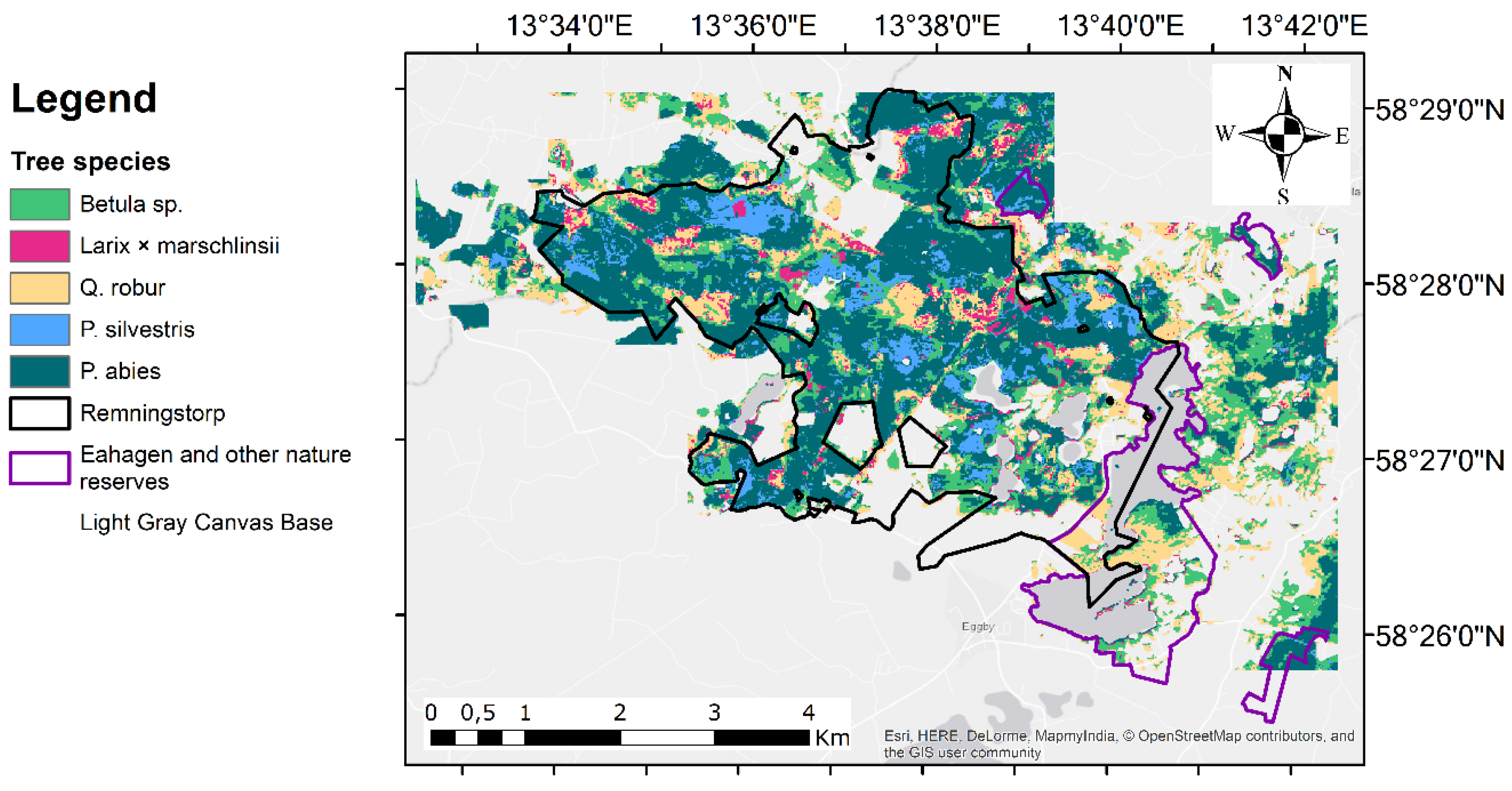
The tree species information classes were limited to the ones shown in Table 1, since the reference data were less extensive for other tree species and forest information classes, such as regeneration or mixed coniferous/deciduous forest. The objective of the study was to investigate the importance of Sentinel-2 image dates and wavelength bands specific to the dominant tree species. Other information classes commonly occurring in land cover classifications (such as water, urban areas, agriculture) were not a focus of this study, and therefore a final map of the area was not the primary aim of this work. However, thematic maps are provided for illustration purposes.
2.3. Satellite Data
To evaluate the effect of combining satellite images from different seasons, a subset of imagery from four dates spread over the vegetation period of 2017 in tile 33VVE was included. Satellite images from 7 April, 27 May, 9 July and 19 October were used. The quality criteria for the images was no or minimal cloud/haze covering the study area, and that the images should be taken at different phenological stages (i.e., before leaf-out to end of senescence) from the same year. Satellite imagery from 2017 was used since they met the criteria better than images from 2016. Phenological data (Table 2) were reviewed to see how the satellite images matched the phenological events in the region. The data originated from the citizen-science-based Swedish National Phenology Network (Svenska fenologinätverket) [20], coordinated by the SLU. Satellite images close to the dates for leaf on-set and senescence were chosen, however, image use is often determined availability of cloud-free images; although Sentinel-2 has a high temporal frequency, there can still be many cloud-contaminated images that cannot be used. The satellite imagery was obtained from the Swea-portal of the Swedish National Space Board website on 20 November 2017. Images with processing Level 1C were readily available (Top Of Atmosphere), which entails that the data have been corrected for radiometric and geometric discrepancies but not for atmospheric [2]. Image pre-processing was carried out in the Sentinel Application Platform [21]. The external plugin Sen2Cor (version 2.3.1) was used to perform the atmospheric correction, which transforms Level 1C Sentinel-2 imagery to Level 2A Bottom of Atmosphere (BoA) reflectance [22].
After the corrections, all 10 remaining bands in each of the four scenes were imported to ArcMap (version 10.5) [23]. The 20 m bands were resampled to 10 m spatial resolution with Nearest Neighbor resampling and merged into a single raster dataset per date. The haze and cloud reduction was assessed by visually comparing the processed image with the non-processed one. Some haze was found in the 19 October image, but not in the other three. Four P. abies plots were covered by haze and were therefore omitted since the haze could have a distorting effect. The geometric correctness was assessed for each image by comparing distinct features in the landscape in each image, but no tendencies for geographic offset were found. A shapefile containing the field plot coordinates was used to see how the cells aligned with the plot boundaries. Data processing was further carried out in the statistical environment R (version 3.4.4) [24]. The satellite images were imported as RasterStacks and the geographic coordinate system was set to SWEREF99TM. The satellite images were later clipped to the extent of the 8 km × 10 km study area. Non-forest land was masked out with FastighetskartanMarkdata GSD vector [25], a land cover map produced by the Swedish National Land Survey.
3. Methods
3.1. Multi-Temporal Imagery
The shapefile containing the plots of the five information classes (Betula sp., Larix × marschlinsii, Q. robur, P. silvestris and P. abies) was imported to R [24]. A weighted average of the spectral values, which corresponded to the area-weighted fraction of each raster cell covered by the 10 m radius plot, was extracted for each individual plot and satellite image and stored in separate data sets. Since relatively homogenous plots have been used in this study, an area-weighted approach was seen as a reasonable assumption. The data set with spectral information from all bands was merged with the associated field data (e.g., information class name) to form the reference data for the RF classifications. Different combinations of image dates were to be tested, and the respective reference data needed for these image date combinations was extracted. To evaluate the multi-temporal approach and the significance of the different image dates, models were fitted for each of the image date combinations presented in Table 3. The 7 April image is abbreviated as A; the 27 May image as M; the 9 July image as J and the 19 October image as O. Abbreviations for combinations of single images were named by adding the single image abbreviations together. The performance of the models was later ranked according to their overall accuracy.
Multi-temporal Sentinel-2 imagery introduces a lot of data which benefits from using a classification method that can deal with multi-dimensional data sets. For this reason, the RF classifier [26] was used to classify the information classes from the satellite data. The RF classifier produces consistently good results as compared to other classification algorithms, is robust, and easy to parameterize [27]. The RF classifier is built by training an ensemble of decision trees (ntree) with samples—drawn with replacement—from the original dataset (i.e., bagging). In each tree, the feature space is stratified into regions by applying splitting-rules on the samples at each node—based on a random sample of predictors (mtry). The measure of the purest split for each predictor at each internal node is the Gini coefficient, which is a measure of variance. At each node, the algorithm chooses the predictor which results in highest Gini value (most homogenous split). Each split results in two daughter-nodes which are subjected to the same process with a new random sample of predictors.
3.2. Data Exploration and Band Importance
Spectral profile plots were constructed for each satellite image as an initial evaluation of the five tree species classes. The band-wise spectral reflectance was averaged for all plots and provides an indication of how each species’ reflectance differs between the wavelength bands and image dates.
It is desirable to produce a model which would exclude correlated variables (i.e., bands) as well as the least predictive bands and furthermore provide a better understanding of the variables that would contribute to high accuracy. The VSURF R-package [30] was used for this purpose, which performs a variable selection on the input data set based on the RF classifier by Breiman [27]. An in-depth description of VSURF is provided in Genuer et al. [31]. The data set containing data from all 40 bands and the information classes for each plot served as input to VSURF.
3.3. Accuracy Assessment
A 10-fold cross-validation was used to evaluate the RF classification models. The input data set was randomly split into 10 samples of equal size. Nine samples (90%) were used to train the classifier and one sample (10%) was used for validation. This was iterated 10 times with random selection and the results were averaged in the confusion matrix. The training and evaluation of the model was carried out with the caret R-package (version 6.0-79) [28].
4. Results
4.1. Multi-Temporal Imagery
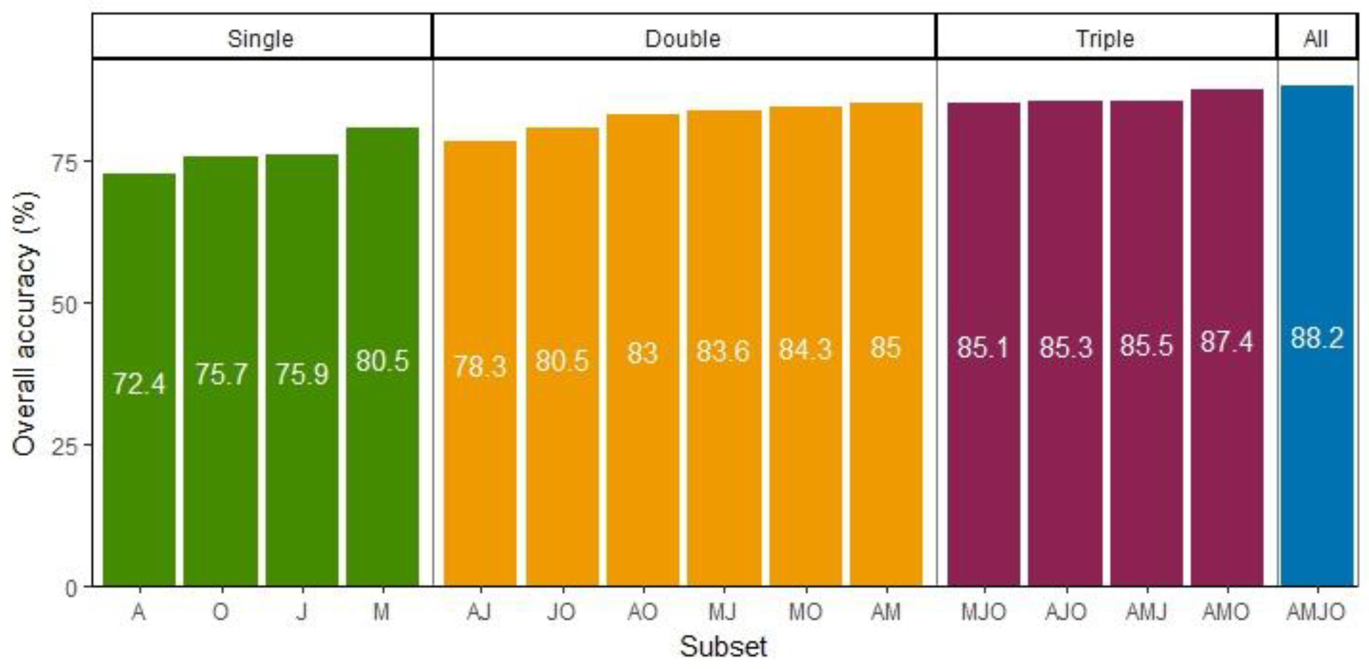
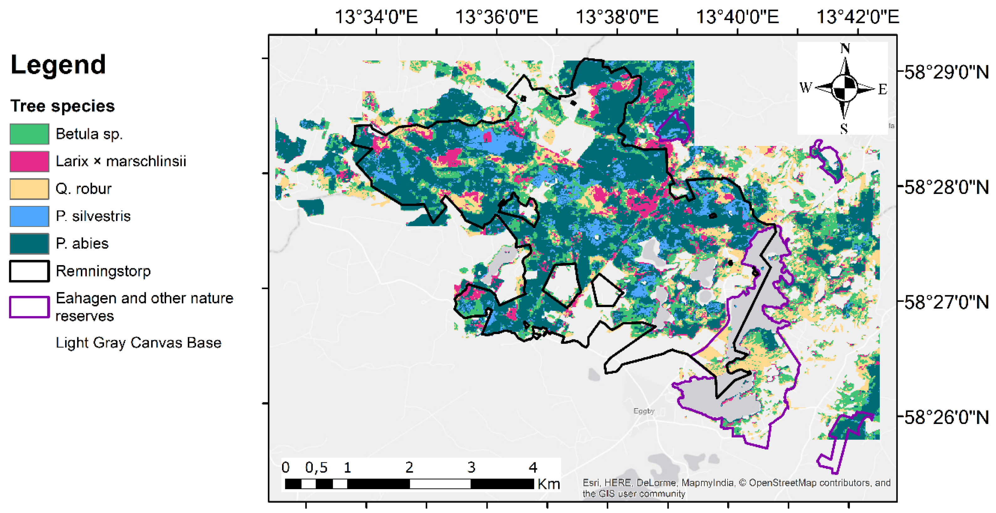
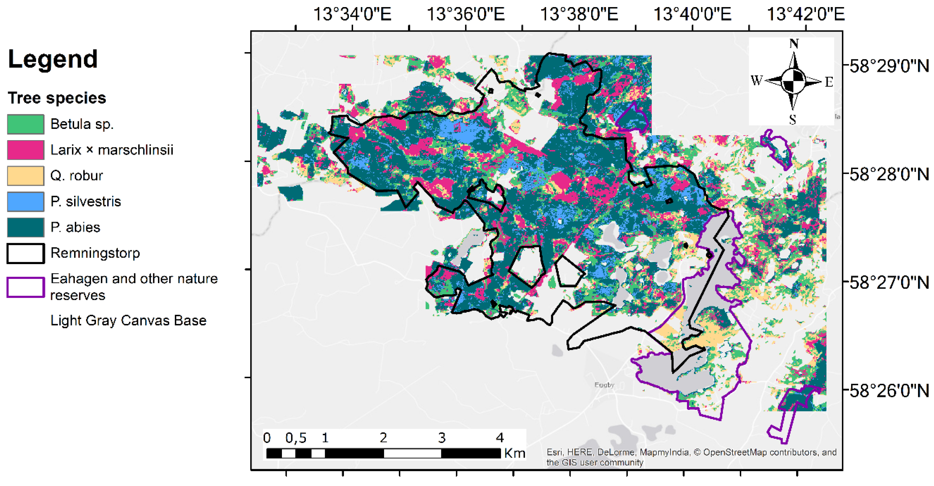
The use of multi-temporal satellite data as opposed to a single date resulted in higher overall accuracy (Figure 2) given that the multi-date image combination included the single date image having the highest accuracy (M = 80.5%; AM = 85%; AMO = 87.4%; AMJO = 88.2%). Single satellite images as input to the RF classifier performed relatively well in classifying tree species, with May producing the highest accuracy (80.5%). The July image was not in the best combination in any of the double and triple image groups, but the April and May images were always in the image combinations with the higher accuracies. Confusion matrices for some of the single date images and the best models in the double and triple image combinations are shown in Appendix A, Table A2, Table A3, Table A4, Table A5, Table A6 and Table A7. Thematic maps for the May image, the VSURF model with 13 bands and the combinations of all images is provided in Appendix A; Figure A1, Figure A2 and Figure A3.
4.2. Tree Species Separation
The confusion matrix of the AMJO model is shown in Table 4. Betula sp., P. abies and Q. robur had higher user’s accuracies than Larix × marschlinsii and P. silvestris. Confusion occurred between P. silvestris with P. abies and between Larix × marschlinsii with Betula sp., hence their lower user’s accuracies.
4.3. Band Importance
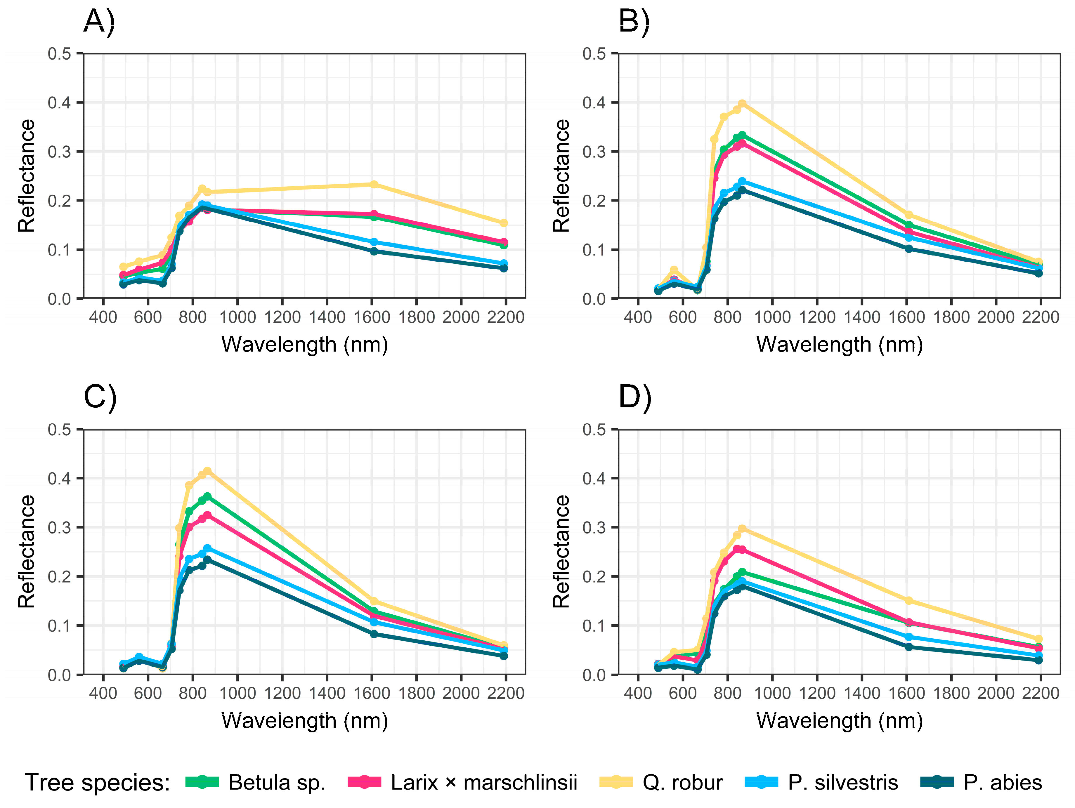
The spectral signatures for each tree species give an indication of how species’ reflectance differs between the wavelength bands and furthermore discloses which bands and what season could aid in the classification. The species-specific change in mean reflectance from one image date to another is illustrated in Figure 3. The 27 May and 9 July images show higher values of spectral reflectance for all tree species in each band compared to the April 4 and 19 October image and the most obvious separation in reflectance is in the red edge spectrum and NIR spectrum. Notably, the three red edge and NIR bands in the May and July images illustrate high separation between the tree species. The SWIR bands in the April and October images also indicate separation.
The variable selection procedure VSURF selected 13 out of 40 bands and they are shown in Appendix A, Table A1, along with their rank. The thematic map is shown in Appendix A, Figure A2. The RF-model built with this band combination led to an overall accuracy of 86.3% and Kappa of 0.82. The confusion matrix for this model was very similar to the AMJO model and is for that reason not shown.
5. Discussion
5.1. Multi-Temporal Imagery
The best model of the different possible combinations was made up of satellite imagery from all dates and all bands with an overall accuracy of 88.2% and a Kappa value of 0.84. The successive addition of a satellite image increased the overall accuracy if the highest performing model in each group was chosen (M → AM → AMO → AMJO). This indicates that additional satellite images complement the spectral information contained in single images and that a multi-temporal data set increases the predictive power of the model. These results align with other studies regarding classifying coniferous and broadleaf forest types conducted in the boreal zone [8,11,12]. Hill et al. [15] used Airborne Thematic Mapper images (2 m pixel size) from March, May, July, September and October for temperate deciduous tree species classification, and found that their well-timed October image acquired during senescence provided good results on its own (71%); when combined with other image dates, higher accuracies were achieved. The highest accuracy (84%) was obtained using a March, July and October combination. In the present study, the May (spring) image had the highest separation between tree species, and higher accuracies were obtained if the May image was combined with an image from any other date. Hill et al. commented that the spring image used in their study was not ideal as far as peak leaf-out conditions were concerned. Zhu et al. [14] obtained the highest accuracy (88.2%) using all image dates. Nelson [8] obtained the highest accuracy using an May/July Sentinel-2 image combination (85.2%), but was not aided by the early senescence image (from late August).
In our study, the overall accuracy plateaued when more images were added or combined. About the same level of overall accuracy was reached for the AMO (87.4%) and the AMJO (88.2%) combination. The July image was redundant, probably since the tree species reflected similarly to the May image and did not contribute additional information. Moreover, the AJO combination had lower overall accuracy (85.3%) than AMO (87.4%). The study by Hill et al. [15] and Zhu et al. [14] had similar results to our study in that the summer image was not among the most important additions, particularly if a well-timed spring and/or fall image was available. The small gain in accuracy between the AMO and AMJO models indicates that the July (summer) image may not be necessary given well-timed images from spring and fall.
The May image performed well on its own and was always in the best combination; this is likely due to the phenological variation between species being highest in late spring. The spectral curves for May and July are similar (Figure 3) but with the May image having a higher reflectance in the green band. That the green band from May was one of the thirteen selected variables may partly explain why the May image was favored over the July image. The April image performed poorly on its own, likely due to leaf-off conditions for some species, however, together with the May image it made up the best model for a two-date combination.
5.2. Performance on Species Level
In this study, Betula sp., Q. robur and P. abies were classified with high user’s accuracies in the AMJO model. Larix × marschlinsii and P. silvestris had lower accuracies and were confused with Betula sp. and Q. robur, and the latter with P. abies. P. silvestris was confused with P. abies which was probably due to P. abies occurring in the understory in some of the field plots. Additionally, P. abies was the most common information class in the AMJO model, which is the class with the highest probability in uncertain cases. The reason for confusion in the case of Larix × marschlinsii is probably due to a small training dataset which—to some degree—failed to provide a coherent spectral reflectance. Interestingly, Larix × marschlinsii has a producer’s accuracy of 100% and a similar pattern is seen for P. silvestris, since only P. abies was misclassified as P. silvestris.
The difference in the confusion matrices for M and AM (Appendix A; Table A3 and Table A6) is that the producer’s accuracies for Betula sp. and Larix × marschlinsii are greatly improved (+11.1% and +22.2%). The reason is that the two species are captured in defoliated condition in April and in leaf-on in May. The AMO combination obtained slightly higher user’s accuracies (Appendix A; Table A7), where Larix × marschlinsii was less confused with Betula sp. and P. abies, probably due to differences in leaf-senescence.
A small number of broadleaved plots were confused with evergreen coniferous and vice versa in the single date images. The reason could be that evergreen coniferous species do not undergo a drastic spectral response change during the year, as compared to deciduous species which drop their leaves due to senescence. The results indicate that evergreen conifers and broadleaves can be better separated in future studies when using a multi-temporal data set.
In contrast with the previously mentioned studies the information classes used in this study did not include mixtures of tree species or other land cover classes. The aim of the present study was to evaluate the temporal and spectral qualities of Sentinel-2 data for the classification of tree species, rather than for complete land cover mapping. However, thematic maps have been provided here for illustrative purposes. In the future, thematic mapping of this area should incorporate more land cover classes, including mixed forest. The results obtained in this study are rather optimistic as they are for homogenous areas of these tree species rather than mixed forest. Mixed forest can vary greatly spectrally and is difficult to classify [16].
5.3. Band Importance
The variable selection excluded 27 of the 40 bands, presumably because they were highly correlated with the 13 bands that were selected. The model built with the 13 selected bands resulted in a similar, although slightly lower, overall accuracy as the AMJO model. Although the accuracies from the AMJO classification are slightly higher than that from the 13 band file, it can be desirable to use variable reduction in order to eliminate correlated variables as well as address a potential Hughes effect where more training data may be needed as more variables are used.
The band ranking in this study conforms with the results obtained in other studies using Sentinel-2 data to some degree. Immitzer et al. [9] and Nelson [8] report that the red edge bands 2, 3 and the narrow NIR band (Sentinel bands 6, 7, and 8a) and SWIR 2 band were among the most important. In this study, the red edge bands 2 and 3 as well as the narrow NIR band 8a were also ranked high and mostly come from the May image, which reinforces the importance of that image. Additionally, most SWIR bands 1 and 2 occur among the 13 highest ranked. However, dissimilarities occur regarding the importance of individual bands in the visible spectrum. Our study shows that the blue band and the green band from May was in the top seven highest ranked bands. The results from Immitzer et al. [9] propose the importance of the blue band, but Nelson [8] reports that the red band was more important, probably since an image from early May was included.
There are some key differences between previous studies and the current one: (i) the timing and processing of the satellite imagery, and (ii) the information classes. The previously mentioned studies [8,9] did not perform atmospheric correction on the satellite imagery to obtain Bottom of Atmosphere (BoA) reflectance, which can have introduced inconsistencies. Nelson [8] omitted some of the most correlated variables, which affected the subset of bands used, and could be more comparable to our results. The information classes were few and no mixed classes were included. It should be kept in mind that this study’s results are specific to the tree species classified; if more tree species were to be included in the classification, additional wavelength bands may then also become important to improve the spectral separation between them [18].
5.4. The Quality of the Field Data
The training data must have a sufficient number of samples (training data set size) to handle the increasing number of dimensions attained by adding predictors and the inter- and intra-species spectral variation. The accuracy of the model will decrease if this is not addressed [30]. Several studies have evaluated the effect of training data set size on land cover classification and on tree species classification [8], using the RF classifier. The results from both studies imply that the classification accuracy increases with the size of the training data set in each class. Nelson [8] reports the lowest accuracy with 10 to 25 plots in each spectral class (77% in overall accuracy) but it increased linearly to 86% if 150 plots were included. Reese [31] reported that 30 to 50 plots per class were enough to represent the spectral variation of individual alpine vegetation classes. The satisfying results in overall accuracy suggest that the training data set was of a sufficient size to account for the spectral variation, particularly over the given study area which is limited in size. The representation of Larix × marschlinsii is one class which may not have had complete spectral representation.
The reference data set used in this study is imbalanced, favoring Norway spruce over the other classes, even after addition of plots to the underrepresented classes. With RF, unbalanced datasets tend to overclassify the most abundant class and therefore misclassify the scarce [32]. Although the problem in modelling is evident, measures to even out the proportion of the classes did not increase the classification accuracy results; to the contrary it may even reduce accuracy [33].
Species-specific basal area >70% was used as a proxy for crown cover on the field plots, which might have introduced some inconsistencies since the relationship between basal area and crown width differs between the species present in this study. Crown cover was not measured during the field inventory and could not be accounted for in the pre-processing of the field data. The threshold of 70% basal area is, however, sufficient to label plots with an information class representing the dominant tree species in each field plot.
The field data did not represent all the development stages for the species used in the classification. The Q. robur field plots originate only from stands with mature trees with fully developed crowns. The other information classes had representation of different age classes, except that young stands that had not reached full crown closure were omitted from the field data since a pure spectral response was preferred. Future studies that focus on larger study areas should aim to represent all development classes in the dataset.
Since the spring of 2017, Sentinel-2 A and B have provided new satellite imagery every two to three days for Sweden, but the occurrence of cloud and haze over the study area resulted in only four usable (cloud-free) images between 1 April and 30 October 2017. The image acquisition time in this study was not optimal since the 7 April image was taken before leaf-onset and the 19 October image is at the end of senescence for all deciduous tree species. The 27 May image proved to have a high significance in the best models in each group.
6. Conclusions
The highest level of overall classification accuracy (88.2%) for the tree species Betula sp., Q. robur, Larix × marschlinsii, P. silvestris and P. abies using Random Forest classification was achieved using all bands from four image dates (7 April, 27 May, 9 July and 19 October, all from 2017) of Sentinel-2 data. The best single date model was from the 27 May image (80.5%), probably due to that it captured the tree species in different phenological stages which gave differing spectral reflectance. The successive addition of a satellite image increased the overall accuracy if the highest performing model in each group was chosen (May ≥ April/May ≥ April/May/October (AMO) ≥ April/May/July/October (AMJO)), although there was little difference between the AMO (87.4%) and AMJO (88.2%) combinations. The 9 July (summer) image was likely too similar to the late May image to add much information. Our results indicated that the inclusion of the July image was not necessary as long as other well-timed spring and/or senescent images were available.
Using all four image dates, the classes Betula sp., Q. robur, Larix × marschlinsii, and P. abies were classified with high user’s accuracies (>85.2%), while P. silvestris had lower accuracy (70.9%). There was very little misclassification occurring between the evergreen conifers and deciduous broadleaf species, which indicates that coniferous and deciduous tree species can be well separated in future studies.
Use of the VSURF variable reduction resulted in selection of 13 of the total 40 wavelength bands, including bands from all image dates; a Random Forest classification of the 13 bands gave an overall accuracy of 86.3%. The red-edge bands (May), the narrow NIR band and most SWIR bands (from all four images) were among the most important variables in the model.
The Sentinel-2 satellite has a high temporal resolution, providing data more frequently than other medium resolution sensors. The frequent image revisit time increases the potential to capture well-timed images with spectral differences between the classes of interest [9,34]. Future studies in the boreo–nemoral region should focus on obtaining imagery from the first part of May (if possible), and also from mid-fall during senescence when there is a gradient in phenological activity. The timing for a species-specific phenological event is dependent on the local climate and the best date will therefore differ depending on location. More accurate observations on leaf out, bloom and senescence in the study area could also be beneficial when selecting appropriate imagery. Furthermore, future studies in this study area could collect more extensive reference data to represent all development stages and more tree species.
Author Contributions
This article is based on the master’s thesis written by M.P. at SLU. M.P. supplemented the field data, pre-processed the data, developed the methodology, interpreted the results and wrote the article. H.R. was the main supervisor, applied for the funding and contributed with developing the methodology and interpreting the results. E.L. was the co-supervisor and compiled the field data. Both have reviewed and commented on the article.
Funding
This article was funded by the Swedish National Space Agency project “Iterative land cover classification using assimilation of multiple Sentinel-2 images with Hidden Markov Models”. DNR 136/15. Heather Reese was the applicant.
Acknowledgments
We give our thanks to the Swedish National Space Agency for the funding of the project and the Ljungberg foundation for providing the technical and logistical basis for students to perform their work in the Ljungberg Remote Sensing lab at SLU.
Conflicts of Interest
The authors declare no conflict of interest. The founding sponsors had no role in the design of the study; in the collection, analyses, or interpretation of data; in the writing of the manuscript, and in the decision to publish the results.
Appendix A

Table A1.
The table shows the bands from the satellite images that were selected in the variable selection procedure using the R-package VSURF. They are listed in ascending order according to their rank.
Table A1.
The table shows the bands from the satellite images that were selected in the variable selection procedure using the R-package VSURF. They are listed in ascending order according to their rank.
| Rank | Band | Date |
|---|---|---|
| 1 | Red edge 2 (B6) | 27 May |
| 2 | SWIR 1 (B11) | 19 October |
| 3 | SWIR 2 (B12) | 7 April |
| 4 | Red edge 3 (B7) | 27 May |
| 5 | Narrow NIR (B8A) | 27 May |
| 6 | Blue (B2) | 27 May |
| 7 | Green (B3) | 27 May |
| 8 | SWIR 1 (B11) | 7 April |
| 9 | SWIR 1 (B11) | 27 May |
| 10 | SWIR 1 (B11) | 9 July |
| 11 | SWIR 2 (B12) | 9 July |
| 12 | Green (B3) | 7 April |
| 13 | Red edge 3 (B7) | 7 April |
Figure A1.
Thematic map of the model including the April, May, July and October image (i.e., AMJO).

Figure A2.
Thematic map of the model including the VSURF model with 13 bands.

Figure A3.
Thematic map of the model including all bands from the May image.

Table A2.
The confusion matrix and the statistical metrics for the model using the April image.
| Reference Data | |||||||
|---|---|---|---|---|---|---|---|
| Betula sp. | Larix × marschlinsii | Q. robur | P. silvestris | P. abies | Total | User’s Accuracy (%) | |
| Betula sp. | 30 | 5 | 5 | 3 | 2 | 45 | 66.7 |
| Larix × marschlinsii | 13 | 11 | 3 | 0 | 0 | 27 | 40.7 |
| Q. robur | 7 | 2 | 28 | 0 | 0 | 37 | 75.7 |
| P. silvestris | 2 | 0 | 0 | 39 | 14 | 55 | 70.9 |
| P. abies | 1 | 0 | 1 | 15 | 81 | 98 | 82.7 |
| Total | 53 | 18 | 37 | 57 | 97 | 262 | |
| Producer’s accuracy (%) | 56.6 | 61.1 | 75.7 | 68.4 | 83.5 | ||
| Overall accuracy (%) | 72.4 | ||||||
| Kappa | 0.64 | ||||||
Table A3.
The confusion matrix and the statistical metrics for the model using the May image.
| Reference Data | |||||||
|---|---|---|---|---|---|---|---|
| Betula sp. | Larix × marschlinsii | Q. robur | P. silvestris | P. abies | Total | User’s Accuracy (%) | |
| Betula sp. | 37 | 1 | 2 | 3 | 2 | 45 | 82.2 |
| Larix × marschlinsii | 5 | 14 | 2 | 2 | 4 | 27 | 51.9 |
| Q. robur | 2 | 0 | 35 | 0 | 0 | 37 | 94.6 |
| P. silvestris | 4 | 3 | 0 | 38 | 10 | 55 | 69.1 |
| P. abies | 4 | 4 | 0 | 7 | 83 | 98 | 84.7 |
| Total | 52 | 22 | 39 | 50 | 99 | 262 | |
| Producer’s accuracy (%) | 71.2 | 63.6 | 89.7 | 76.0 | 83.8 | ||
| Overall accuracy (%) | 80.5 | ||||||
| Kappa | 0.74 | ||||||
Table A4.
The confusion matrix and the statistical metrics for the model using the July image.
| Reference Data | |||||||
|---|---|---|---|---|---|---|---|
| Betula sp. | Larix × marschlinsii | Q. robur | P. silvestris | P. abies | Total | User’s Accuracy (%) | |
| Betula sp. | 35 | 2 | 4 | 1 | 3 | 45 | 77.8 |
| Larix × marschlinsii | 8 | 9 | 2 | 5 | 3 | 27 | 33.3 |
| Q. robur | 4 | 1 | 32 | 0 | 0 | 37 | 86.5 |
| P. silvestris | 1 | 2 | 0 | 40 | 12 | 55 | 72.7 |
| P. abies | 3 | 5 | 0 | 7 | 83 | 98 | 84.7 |
| Total | 51 | 19 | 38 | 53 | 101 | 262 | |
| Producer’s accuracy (%) | 68.6 | 47.4 | 84.2 | 75.5 | 82.2 | ||
| Overall accuracy (%) | 75.9 | ||||||
| Kappa | 0.68 | ||||||
Table A5.
The confusion matrix and the statistical metrics for the model using the October image.
| Reference Data | |||||||
|---|---|---|---|---|---|---|---|
| Betula sp. | Larix × marschlinsii | Q. robur | P. silvestris | P. abies | Total | User’s Accuracy (%) | |
| Betula sp. | 35 | 0 | 6 | 1 | 3 | 45 | 77.8 |
| Larix × marschlinsii | 5 | 11 | 1 | 4 | 6 | 27 | 40.7 |
| Q. robur | 7 | 1 | 29 | 0 | 0 | 37 | 78.4 |
| P. silvestris | 3 | 2 | 2 | 39 | 9 | 55 | 70.9 |
| P. abies | 2 | 5 | 0 | 9 | 82 | 98 | 83.7 |
| Total | 52 | 19 | 38 | 53 | 100 | 262 | |
| Producer’s accuracy (%) | 67.3 | 57.9 | 76.3 | 73.6 | 82.0 | ||
| Overall accuracy (%) | 75.7 | ||||||
| Kappa | 0.68 | ||||||
Table A6.
The confusion matrix and the statistical metrics for the model using the April and May images.
Table A6.
The confusion matrix and the statistical metrics for the model using the April and May images.
| Reference Data | |||||||
|---|---|---|---|---|---|---|---|
| Betula sp. | Larix × marschlinsii | Q. robur | P. silvestris | P. abies | Total | User’s Accuracy (%) | |
| Betula sp. | 42 | 2 | 0 | 0 | 1 | 45 | 93.3 |
| Larix × marschlinsii | 5 | 20 | 2 | 0 | 0 | 27 | 74.1 |
| Q. robur | 2 | 0 | 35 | 0 | 0 | 37 | 94.6 |
| P. silvestris | 3 | 0 | 0 | 41 | 11 | 55 | 74.5 |
| P. abies | 4 | 0 | 0 | 8 | 86 | 98 | 87.8 |
| Total | 56 | 22 | 37 | 49 | 98 | 262 | |
| Producer’s accuracy (%) | 75.0 | 90.9 | 94.6 | 83.7 | 87.8 | ||
| Overall accuracy (%) | 85.0 | ||||||
| Kappa | 0.80 | ||||||
Table A7.
The confusion matrix and the statistical metrics for the model using the April, May and October images.
Table A7.
The confusion matrix and the statistical metrics for the model using the April, May and October images.
| Reference Data | |||||||
|---|---|---|---|---|---|---|---|
| Betula sp. | Larix × marschlinsii | Q. robur | P. silvestris | P. abies | Total | User’s Accuracy (%) | |
| Betula sp. | 42 | 1 | 1 | 0 | 1 | 45 | 93.3 |
| Larix × marschlinsii | 4 | 21 | 2 | 0 | 0 | 27 | 77.8 |
| Q. robur | 2 | 0 | 35 | 0 | 0 | 37 | 94.6 |
| P. silvestris | 1 | 0 | 0 | 43 | 11 | 55 | 78.2 |
| P. abies | 3 | 0 | 0 | 5 | 90 | 98 | 91.8 |
| Total | 52 | 22 | 38 | 48 | 102 | 262 | |
| Producer’s accuracy (%) | 80.8 | 95.5 | 92.1 | 89.6 | 88.2 | ||
| Overall accuracy (%) | 87.4 | ||||||
| Kappa | 0.83 | ||||||
References
- FSC Sweden. Swedish FSC Standard for Forest Certification Including SLIMF Indicators; FSC Sweden: Uppsala, Sweden, 2017. [Google Scholar]
- Drusch, M.; Del Bello, U.; Carlier, S.; Colin, O.; Fernandez, V.; Gascon, F.; Hoersch, B.; Isola, C.; Laberinti, P.; Martimort, P.; et al. Sentinel-2: ESA’s Optical High-Resolution Mission for GMES Operational Services. Remote Sens. Environ. 2012, 120, 25–36. [Google Scholar] [CrossRef]
- Clark, M.L.; Roberts, D.A. Species-Level Differences in Hyperspectral Metrics among Tropical Rainforest Trees as Determined by a Tree-Based Classifier. Remote Sens. 2012, 4, 1820–1855. [Google Scholar] [CrossRef]
- Ustin, S.L.; Gitelson, A.A.; Jacquemoud, S.; Schaepman, M.; Asner, G.P.; Gamon, J.A.; Zarco-Tejada, P. Retrieval of foliar information about plant pigment systems from high resolution spectroscopy. Remote Sens. Environ. 2009, 113, S67–S77. [Google Scholar] [CrossRef] [Green Version]
- Clark, M.; Roberts, D.; Clark, D. Hyperspectral discrimination of tropical rain forest tree species at leaf to crown scales. Remote Sens. Environ. 2005, 96, 375–398. [Google Scholar] [CrossRef]
- Asner, G.P. Biophysical and Biochemical Sources of Variability in Canopy Reflectance. Remote Sens. Environ. 1998, 64, 234–253. [Google Scholar] [CrossRef]
- Boyd, D.S.; Danson, F.M. Satellite remote sensing of forest resources: Three decades of research development. Prog. Phys. Geogr. 2005, 29, 1–26. [Google Scholar] [CrossRef]
- Nelson, M. Evaluating Multitemporal Sentinel-2 Data for Forest Mapping Using Random Forest; Stockholm University: Diva, Sweden, 2017. [Google Scholar]
- Immitzer, M.; Vuolo, F.; Atzberger, C. First Experience with Sentinel-2 Data for Crop and Tree Species Classifications in Central Europe. Remote Sens. 2016, 8, 166. [Google Scholar] [CrossRef]
- Mickelson, J.G.; Civco, D.L.; Silander, J.A. Delineating forest canopy species in the northeastern United States using multi-temporal TM imagery. Am. Soc. Photogramm. Remote Sens. 1998, 64, 891–904. [Google Scholar]
- Reese, H.M.; Lillesand, T.M.; Nagel, D.E.; Stewart, J.S.; Goldmann, R.A.; Simmons, T.E.; Chipman, J.W.; Tessar, P.A. Statewide land cover derived from multiseasonal Landsat TM data: A retrospective of the WISCLAND project. Remote Sens. Environ. 2002, 82, 224–237. [Google Scholar] [CrossRef]
- Wolter, P.; Mladenoff, D.J. Improved Forest Classification in the Northern Lake States Using Multi-Temporal Landsat Imagery. Photogramm. Eng. Remote Sens. 1995, 61, 1129–1143. [Google Scholar]
- Schriever, J.R.; Congalton, R.G. Evaluating seasonal variability as an aid to cover-type mapping from Landsat Thematic Mapper data in the northeast. Photogramm. Eng. Remote Sens. 2005, 3, 321–327. [Google Scholar]
- Zhu, X.L.; Liu, D.S. Accurate mapping of forest types using dense seasonal Landsat time-series. ISPRS J. Photogramm. Remote Sens. 2014, 96, 1–11. [Google Scholar] [CrossRef]
- Hill, R.A.; Wilson, A.K.; George, M.; Hinsley, S.A. Mapping tree species in temperate deciduous woodland using time-series multi-spectral data. Appl. Veg. Sci. 2010, 13, 86–99. [Google Scholar] [CrossRef]
- Reese, H.; Nilsson, M.; Pahlén, T.G.; Hagner, O.; Joyce, S.; Tingelöf, U.; Egberth, M.; Olsson, H. Countrywide estimates of forest variables using satellite data and field data from the national forest inventory. AMBIO J. Hum. Environ. 2003, 32, 542–548. [Google Scholar] [CrossRef]
- Dalponte, M.; Orka, H.O.; Gobakken, T.; Gianelle, D.; Naesset, E. Tree Species Classification in Boreal Forests with Hyperspectral Data. IEEE Trans. Geosci. Remote Sens. 2013, 51, 2632–2645. [Google Scholar] [CrossRef]
- Immitzer, M.; Atzberger, C.; Koukal, T. Tree Species Classification with Random Forest Using Very High Spatial Resolution 8-Band WorldView-2 Satellite Data. Remote Sens. 2012, 4, 2661–2693. [Google Scholar] [CrossRef] [Green Version]
- Nilsson, M. SLU Forest Map. In The Swedish National Forest Inventory; Department of Forest Resource Management: Umeå, Sweden, 2018. [Google Scholar]
- Bolmgren, K. Naturkalendern. Svenska Fenologinätverket; Swedish University of Agricultural Sciences (SLU): Uppsala, Sweden, 2017. [Google Scholar]
- Sentinel Application Plattform (SNAP), 5.0.0; Brockmann Consult, Array Systems Computing and C-S: 2018. Available online: https://forum.step.esa.int (accessed on 22 October 2018).
- Mueller-Wilm, U. Sen2Cor Configuration and User Manual; European Space Agency (ESA): Paris, France, 2017. [Google Scholar]
- Enviromental Science Research Institute ArcGIS Desktop; 10.5; ESRI: Redlands, CA, USA, 2017.
- R Development Core Team. R: A Language and Environment for Statistical Computing 3.4.4; R Foundation for Statistical Computing: Vienna, Austria, 2018. [Google Scholar]
- GSD-Fastighetskartan vektor. Lantmäteriet, Gävle, Sweden. 2017. Available online: https://zeus.slu.se/get/ (accessed on 22 October 2018).
- Breiman, L. Random Forests. Mach. Learn. 2001, 45, 5–32. [Google Scholar] [CrossRef] [Green Version]
- Belgiu, M.; Drăguţ, L. Random forest in remote sensing: A review of applications and future directions. ISPRS J. Photogramm. Remote Sens. 2016, 114, 24–31. [Google Scholar] [CrossRef]
- Kuhn, M. Package ‘caret’, Classification and Regression Training. J. Stat. Softw. 2008, 28, 1–26. [Google Scholar]
- Kuhn, M. Building Predictive Models in R Using the caret Package. J. Stat. Softw. 2008, 28, 1–26. [Google Scholar] [CrossRef]
- Hughes, G. On the mean accuracy of statistical pattern recognizers. IEEE Trans. Inf. Theory 1968, 14, 55–63. [Google Scholar] [CrossRef]
- Reese, H. Classification of Sweden’s Forest and Alpine Vegetation Using Optical Satellite and Inventory Data. Doctoral’s Thesis, Sveriges lantbruksuniversitet, Umeå, Sweden, 2011. [Google Scholar]
- Chen, C.; Liaw, A.; Breiman, L. Using Random Forest to Learn Imbalanced Data. Tech Report 2004, 12, 1–12. [Google Scholar]
- Zhu, Z.; Gallant, A.L.; Woodcock, C.E.; Pengra, B.; Olofsson, P.; Loveland, T.R.; Jin, S.; Dahal, D.; Yang, L.; Auch, R.F. Optimizing selection of training and auxiliary data for operational land cover classification for the LCMAP initiative. ISPRS J. Photogram. Remote Sens. 2016, 122, 206–221. [Google Scholar] [CrossRef]
- Vuolo, F.; Neuwirth, M.; Immitzer, M.; Atzberger, C.; Ng, W.-T. How much does multi-temporal Sentinel-2 data improve crop type classification? Int. J. Appl. Earth Obs. Geoinf. 2018, 72, 122–130. [Google Scholar] [CrossRef]
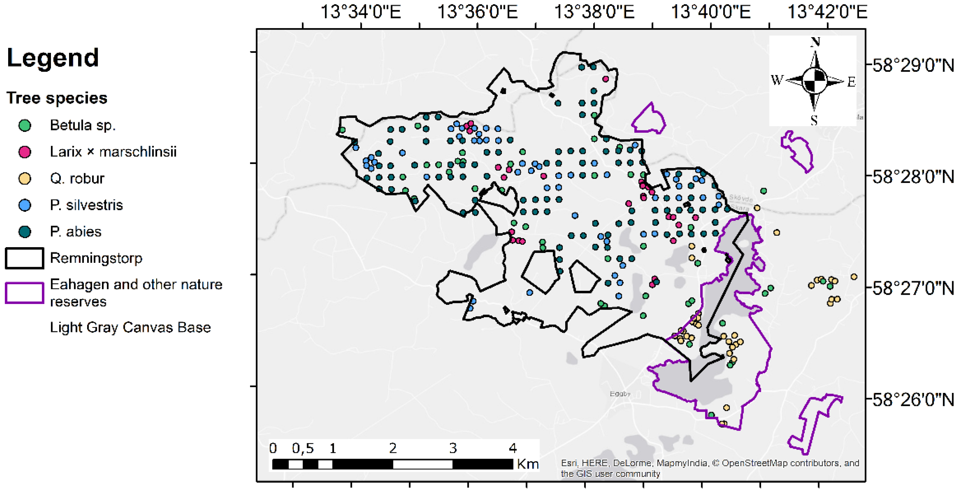
Figure 1.
Map of the study area showing the field plots in Remningstorp, Eahagen and in the nearby stands. Each color represents one of the five information classes (tree species).
Figure 1.
Map of the study area showing the field plots in Remningstorp, Eahagen and in the nearby stands. Each color represents one of the five information classes (tree species).

Figure 2.
The overall accuracy (%) for individual RF models produced using all bands for single image, and multiple image combinations. The colors represent the number of satellite images used and the single letters indicate the image date: A = 7 April; M = 27 May; J = 9 July; O = 19 October.
Figure 2.
The overall accuracy (%) for individual RF models produced using all bands for single image, and multiple image combinations. The colors represent the number of satellite images used and the single letters indicate the image date: A = 7 April; M = 27 May; J = 9 July; O = 19 October.

Figure 3.
The mean spectral reflectance for each tree species illustrated for each image date: (A) 7 April, (B) 27 May, (C) 9 July and (D) 19 October. The data come from the extracted spectral information from the field plots.
Figure 3.
The mean spectral reflectance for each tree species illustrated for each image date: (A) 7 April, (B) 27 May, (C) 9 July and (D) 19 October. The data come from the extracted spectral information from the field plots.

Table 1.
Summary of the reference data used in the classifications. The number of field plots is presented by tree species and data collection method.
Table 1.
Summary of the reference data used in the classifications. The number of field plots is presented by tree species and data collection method.
| Tree Species | Field Inventory 1 1 | Field Inventory 2 2 | Aerial Photo Interpretation | Total |
|---|---|---|---|---|
| Betula sp. | 24 | 3 | 18 | 45 |
| Larix × marschlinsii | 3 | 24 | 27 | |
| Q. robur | 17 | 20 | 37 | |
| P. silvestris | 27 | 28 | 55 | |
| P. abies | 98 | 98 | ||
| Total (Proportion) | 169 (64.5%) | 23 (8.8%) | 70 (26.7%) | 262 |
1 The field inventory carried out in 2016/2017 with systematic sampling design. 2 The field inventory carried out in the fall of 2017 by placing out subjective plots.
Table 2.
Phenology data for the five tree species in the study. The closest geographical observation for each tree species and type is presented.
Table 2.
Phenology data for the five tree species in the study. The closest geographical observation for each tree species and type is presented.
| Tree Species | Leaf-Onset | Bloom | Senescence | Shoot Elongation (Conifers) |
|---|---|---|---|---|
| Betula sp. | 26 May 2017 | 2 June 2017 | 9 October 2017 | - |
| Larix × marschlinsii | 30 April 2017 | 4 May 2017 | 30 September 2017 | - |
| Q. robur | 13 May 2017 | - | - | - |
| P. silvestris | - | - | - | 19 May 2017 |
| P. abies | - | - | - | 21 May 2017 |
Table 3.
The different combinations of satellite imagery for which Random Forest (RF)-models were fitted.
Table 3.
The different combinations of satellite imagery for which Random Forest (RF)-models were fitted.
| Group | Subset | Abbreviation | Number of Bands |
|---|---|---|---|
| Single | 7 April | A | 10 |
| 19 October | O | 10 | |
| 9 July | J | 10 | |
| 27 May | M | 10 | |
| Double | 7 April/9 July | AJ | 20 |
| 9 July/19 October | JO | 20 | |
| 7 April/19 October | AO | 20 | |
| 27 May/9 July | MJ | 20 | |
| 27 May/19 October | MO | 20 | |
| 7 April/27 May | AM | 20 | |
| Triple | 27 May/9 July/19 October | MJO | 30 |
| 7 April/9 July/19 October | AJO | 30 | |
| 7 April/27 May/9 July | AMJ | 30 | |
| 7 April/27 May/19 October | AMO | 30 | |
| All | 7 April/27 May/9 July/19 October | AMJO | 40 |
Table 4.
The confusion matrix and the statistical metrics for the model with all four satellite images (i.e., 7 April/27 May/9 July/19 October (AMJO)).
Table 4.
The confusion matrix and the statistical metrics for the model with all four satellite images (i.e., 7 April/27 May/9 July/19 October (AMJO)).
| Reference Data | |||||||
|---|---|---|---|---|---|---|---|
| Betula sp. | Larix × marschlinsii | Q. robur | P. silvestris | P. abies | Total | User’s Accuracy (%) | |
| Betula sp. | 43 | 0 | 1 | 0 | 1 | 45 | 95.6 |
| Larix × marschlinsii | 2 | 23 | 2 | 0 | 0 | 27 | 85.2 |
| Q. robur | 1 | 0 | 36 | 0 | 0 | 37 | 97.3 |
| P. silvestris | 3 | 0 | 0 | 39 | 13 | 55 | 70.9 |
| P. abies | 3 | 0 | 0 | 6 | 89 | 98 | 90.8 |
| Total | 52 | 23 | 39 | 45 | 103 | 262 | |
| Producer’s accuracy (%) | 82.7 | 100.0 | 92.3 | 86.7 | 86.4 | ||
| Overall accuracy (%) | 88.2 | ||||||
| Kappa | 0.84 | ||||||
© 2018 by the authors. Licensee MDPI, Basel, Switzerland. This article is an open access article distributed under the terms and conditions of the Creative Commons Attribution (CC BY) license (http://creativecommons.org/licenses/by/4.0/).
Share and Cite
MDPI and ACS Style
Persson, M.; Lindberg, E.; Reese, H. Tree Species Classification with Multi-Temporal Sentinel-2 Data. Remote Sens. 2018, 10, 1794. https://doi.org/10.3390/rs10111794
AMA Style
Persson M, Lindberg E, Reese H. Tree Species Classification with Multi-Temporal Sentinel-2 Data. Remote Sensing. 2018; 10(11):1794. https://doi.org/10.3390/rs10111794
Chicago/Turabian StylePersson, Magnus, Eva Lindberg, and Heather Reese. 2018. "Tree Species Classification with Multi-Temporal Sentinel-2 Data" Remote Sensing 10, no. 11: 1794. https://doi.org/10.3390/rs10111794
Note that from the first issue of 2016, this journal uses article numbers instead of page numbers. See further details here.