Long-Term Arctic Snow/Ice Interface Temperature from Special Sensor for Microwave Imager Measurements


1
School of Earth and Environmental Sciences, Seoul National University, Seoul 08826, Korea
2
Department of Atmospheric Science, Colorado State University, Fort Collins, CO 80523, USA
*
Author to whom correspondence should be addressed.
Remote Sens. 2018, 10(11), 1795; https://doi.org/10.3390/rs10111795
Submission received: 22 August 2018
/
Revised: 2 October 2018
/
Accepted: 9 November 2018
/
Published: 12 November 2018
(This article belongs to the Special Issue Remote Sensing of Essential Climate Variables and Their Applications)
Abstract
:The Arctic sea ice region is the most visible area experiencing global warming-induced climate change. However, long-term measurements of climate-related variables have been limited to a small number of variables such as the sea ice concentration, extent, and area. In this study, we attempt to produce a long-term temperature record for the Arctic sea ice region using Special Sensor for Microwave Imager (SSM/I) Fundamental Climate Data Record (FCDR) data. For that, we developed an algorithm to retrieve the wintertime snow/ice interface temperature (SIIT) over the Arctic Ocean by counting the effect of the snow/ice volume scattering and ice surface roughness on the apparent emissivity (the total effect is referred to as the correction factor). A regression equation was devised to predict the correction factor from SSM/I brightness temperatures (TBs) only and then applied to SSM/I 19.4 GHz TB to estimate the SIIT. The obtained temperatures were validated against collocated Cold Regions Research and Engineering Laboratory (CRREL) ice mass balance (IMB) drifting buoy-measured temperatures at zero ice depth. It is shown that the SSM/I retrievals are in good agreement with the drifting buoy measurements, with a correlation coefficient of 0.95, bias of 0.1 K, and root-mean-square error of 1.48 K on a daily time scale. By applying the algorithm to 24-year (1988–2011) SSM/I FCDR data, we were able to produce the winter-time temperature at the sea ice surface for the 24-year period.

1. Introduction
The increasing emission of man-made greenhouse gases has caused global warming of 0.8 °C since 1900 [1,2,3], but the temperature increase is not the same everywhere over the globe. Especially, over the Arctic polar region, where snow and ice cover the ocean, the increase in the near-surface is nearly twice that in the tropics–a phenomenon called Arctic amplification [4,5]. Such a rapidly rising surface temperature over the Arctic is manifested by changes in the sea ice extent over last three decades. The sea ice extent has been declining at a rate of ≈3.8%/decade [6]. The largest decline is observed in September with an alarming rate of ≈13%/decade, corresponding to more than 30% of sea ice loss compared with the late 1970s [7,8].
The impact of ice loss appears to be profound, not only influencing the local climate, hydrological cycle, ecosystems, and natural habitats, but also affecting the global weather/climate system. With the declining sea ice, more ocean water will be exposed to cold and windy atmospheric environments, probably inducing enhanced evaporation to the cold atmosphere, which can lead to more water vapor, clouds, and more precipitation [9]. The precipitation change in response to the sea ice melt is particularly interesting because the precipitation itself (regardless of snow or rain) has the potential to feedback the climate [10]. As expected, increased precipitation is noted in the Arctic [11], mainly due to the increased local evaporation caused by the sea ice loss [12]. Furthermore, a higher percentage of precipitation throughout the Arctic summer time will be in liquid form, namely rain, due to the warmer low atmosphere, forcing the snow cover to further decline [10]. It is projected that rain will be the dominant form of precipitation in the Arctic by the end of the 21st century [13]. The increased rain, a hydrological response to dramatically decreasing sea ice (or to the warming atmosphere) should lead to a positive feedback to ice melting, through the substantially decreasing surface albedo, establishes a self-feeding cycle where warming temperatures will lead to more rain and ice melt [10] and cause more warming due to even more rain and ice melt.
With respect to the influence of the decline of Arctic sea ice on the weather/climate elsewhere, there is cumulating evidence that Arctic warming has been identified as an important element of the variability of mid-latitude, large-scale atmospheric circulation including storm tracks, planetary waves, jet stream, and energy transport [14,15]. It is reported that the atmospheric variability due to Arctic warming is closely linked to more frequent events of atmospheric blocking patterns [16] and increased cold surges with snowy winters in East Asia, Europe, and Northern America [14,17,18]. Central and northern Europe have experienced six years (2007–2012) of extraordinary wet summer, likely due to the southward shift of the summer jet forced by Arctic sea ice loss [19]. More extreme weather may be expected worldwide in the future due to continuous Arctic warming and the associated sea ice loss.
Although current monitoring of sea ice extent and understanding of subsequent impacts on climate components are in high confidence, dramatic changes of the Arctic climate system and expected continuous change in the future make it difficult to assess the future evolution of Arctic environments and/or predict global climate change. To facilitate our understanding of Arctic climate change and thus to reduce the uncertainty of future climate change assessment, observations of climate variables, such as the sea ice extent and its depth, snow cover, and depth are needed, in addition to observations of thermal structures throughout the atmosphere-snow-ice column. At least, much needed thermodynamic variables may be the surface air temperature, snow top temperature, and snow-ice interface temperature (SIIT), from which the thermal structure of the snow-ice system can be studied and related to the sea ice melt or sea ice depth change. The SIIT is intriguing because, if ice depth is known, the heat content of an ice column can be calculated by assuming a nearly constant lapse rate within the ice layer, at least during winter. The amount of heat content held by the ice should be the main factor controlling upward heat transfer from the ocean water to the atmosphere. It builds up a preconditioning of how fast the ice melts in spring and summer, or how fast the ice grows in fall and winter. Thus, the SIIT is valuable information, which can lead to better climate monitoring over the Arctic. In fact, the aforementioned sea ice decline, changes in the Arctic hydrological cycle, and influences on the mid-latitude weather are all related to the SIIT because the SIIT is the variable that can give information on the thermal state of the ice.
In this study, we propose an algorithm to produce the long-term SIIT from SSM/I microwave (MW) measurements, which can penetrate the snow layer without much interference. A recent study showed that 6.9 GHz brightness temperature (TB) measurements are theoretically related to the sea ice emissivity and temperature [20]. Although the retrieved ice temperature from 6.9 GHz TBs is in good agreement with the buoy-measured SIIT, the acquisition of long-term data may not be possible, because 6.9 GHz TB measurements before the launch of the Advanced Microwave Scanning Radiometer–EOS (AMSR-E) in August 2002 are not available.
In reality, long-term global MW observations are available, as shown in the intercalibrated Fundamental Climate Data Record (FCDR) of TBs [21], covering more than 30 years, but without the 6.9 GHz channel. In the higher frequency region, such as 19.4 GHz, it is difficult to apply the Fresnel assumption for the emissivity retrieval due to surface and volume scatterings. However, if the influences of surface and volume scatterings are known and included in the radiative transfer calculation within the sea ice, it may be possible to retrieve the temperature even using higher frequencies.
Aiming at producing long-term SIIT over the Arctic sea ice, we develop an algorithm for retrieving the SIIT from SSM/I TB data, by counting surface and volume scattering effects on the measured TBs, which were examined in the previous study [22]. For this objective, we introduce a correction factor to remove surface and volume scattering influences from measured TBs. Subsequently, the radiative transfer equation is solved for the physical emission temperature from SSM/I (or SSMIS alike) TBs only using the correction factor and combined Fresnel equation. Based on this methodology, we attempt to produce long-term sea ice temperature over the Arctic. The obtained long-term SIIT will certainly help to understand how the global warming has influenced the Arctic climate change in the past decades.
2. Used Data
2.1. Passive MW Data
In this study, we use FCDR SSM/I 19.4 and 37.0 GHz vertically and horizontally polarized TBs to retrieve the sea ice temperature. The SSM/I sensors have measured MW TBs with a viewing angle near 53° since 1987. The sensors aboard different platforms are physically consistent but depend on varying orbital and navigational quantities such as the incident angle, resolution, and observation time. The objective of SSM/I FCDR data is to generate consistent and well-calibrated MW TBs from 1987 onwards by using multiple techniques for intercalibration [21,23]. In this study, these SSM/I FCDR orbital data were converted to 25 km Equal-Area Scalable Earth (EASE)-grid data, on a daily basis, to collocate SSM/I data with gridded AMSR-E TBs and SSM/I bootstrap sea ice concentration data [24]. More information on the SSM/I FCDR dataset can be found in References [21,23] and on the webpage of the Precipitation Research Group of the Department of Atmospheric Science of the Colorado State University (http:/rain.atmos.colostate.edu/FCDR/).
The AMSR-E 6.9 GHz TBs are used for retrieving the adjusted real refractive index and emitting layer temperature of Arctic sea ice, adapting a method described in Reference [20]. Level 3 daily TBs at 6.9 GHz were obtained from the Global Change Observation Mission (GCOM) data center site (http://gcom-w1.jaxa.jp/). In addition, bootstrap sea ice concentration data are applied to minimize the influences of water contamination. When sea ice coexists with open water within the same pixel, a heterogeneous problem arises in the interpretation of the MW brightness temperature, making the retrieval difficult. In this study, we minimized the water contamination effect in the retrieval by imposing 98% of sea ice concentration as a criterion. Sea ice concentration data were downloaded from the National Snow and Ice Data Center (NSIDC) website (http://nsidc.org/) [24].
2.2. CRREL Buoy Measurements
To validate the developed algorithm, we compared the pixel-based retrieved sea ice temperature with in situ measurements from U.S. Navy Cold Regions Research and Engineering Laboratory (CRREL) ice mass balance (IMB) buoy measurements at a daily time scale [25]. The buoy incorporates a thermometer string instrument to measure the temperature profile from the near-surface atmosphere, through the sea ice, and to sea water. In addition, the snow depth and sea ice thickness are measured with an acoustic sounder installed at the buoy. Daily averages were taken from 2-hourly measured data, which were downloaded from the CRREL website (http://imb-crrel-dartmouth.org/imb.crrel/). Temperature at zero ice depth (which is also referred to as SIIT but from buoy measurement) is used for the comparison with collocated SSM/I-derived SIIT.
Two types of CRREL IMB buoy data are available, i.e., “Provisional Buoy” data and “Archived Buoy” data. The “Provisional Buoy” data were archived without quality control, and thus often abnormal features are found in the “Provisional Buoy” data, i.e., (1) the air temperature is substantially higher than snow/ice interface (or zero ice depth) temperature even during the winter time; (2) a strong inversion layer exists within the sea ice; (3) the air temperature variation is smaller than that of temperature at zero ice depth; and (4) the air/snow interface or at snow/ice interface show no vertical temperature gradient change. The “Archived Buoy” data are quality-controlled, but, even some of “Archived Buoy” data show abnormal features similar to that found in the “Provisional Buoy” data, although there are relatively few cases. In this study, we only used “Archived Buoy” data for the comparison because of the abnormal features found in “Provisional Buoy” data. However, more control checks are necessary even for “Archived Buoy” data, and we apply quality assurance checks (1)–(4) to “Archived Buoy” data before the comparison. Details of the quality checks are provided in Section 4.
3. Theoretical Background and Methodology
The theoretical background for the algorithm development was developed and introduced in a previous study ([22], this reference, (Lee, Sohn, and Shi, 2018), is now referred to as LSS18). Here, we provide a summary of the theoretical backgrounds used in that study, and an algorithm development for SSM/I measurements. Detailed explanations are provided in Appendix A.
3.1. Simple Snow/Ice Model for Radiative Transfer
In this study, sea ice used for the radiative transfer is composed of three layers, i.e., a snow layer at the top, surface ice layer (or freeboard sea ice layer) in the middle below the snow layer, and congelation ice layer as the lowest layer [26]. The snow layer (top layer) and upper part of the surface ice layer (middle layer) are presumed to be the volume scattering layer that attenuates the radiation emanating from the emission layer below. The model has one emission layer with temperature and related emissivity (TE and ε, respectively). The emission layer is located below the volume scattering layer and composed of the lower part of the surface ice layer and/or upper part of the congelation ice layer (see Figure 1 in Reference [22]). For the radiative transfer, surface and volume scatterings occurring above the emission layer are treated independent of the emission layer, not allowing interactions between the two layers.
If TBsfc is defined as an upwelling TB at the snow top, then the radiative transfer through the snow-ice layer can be expressed as follows:
where τsca is the optical thickness associated with the snow/ice volume scattering.
3.2. Apparent Emissivity
We defined the apparent emissivity () by taking the ratio between TE and TBsfc:
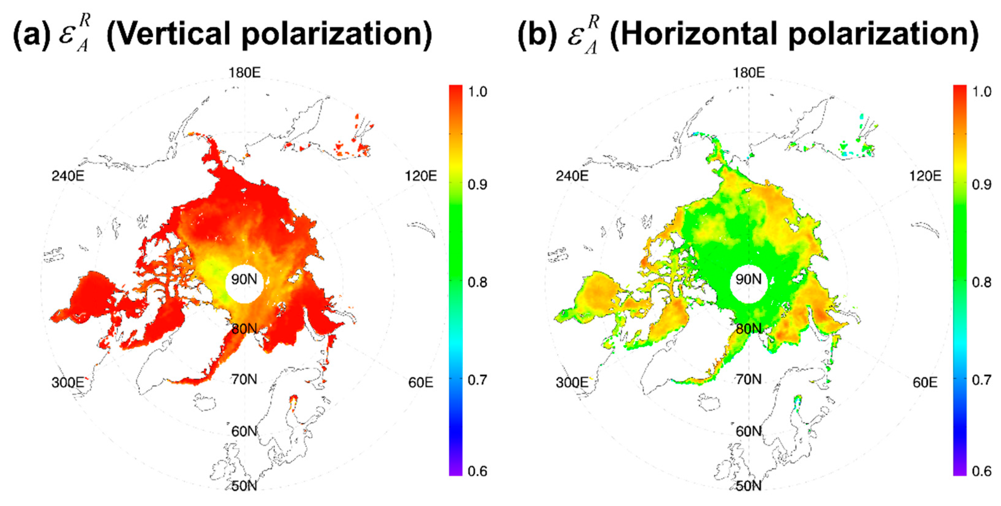
Apparent emissivities at the SSM/I 19.4 GHz channels are obtained by taking the ratio of SSM/I 19.4 GHz TBsfc to the sea ice emission temperature (TE), according to Equation (2). TBsfc here is from the measured TB after removing atmospheric effects, which are calculated using the line-by-line radiative transfer model of the Satellite Data Simulator Unit (SDSU)-version 2.1 [27] with inputs of atmospheric temperature and humidity profiles from European Centre for Medium-Range Weather Forecasts Reanalysis (ERA)-Interim data [28]. The collocated TE is obtained from the AMSR 6.9 GHz retrieved SIIT, based on the finding that its emission weighting function is similar to that for 19.4 GHz. Figure 1 shows the spatial distributions of the apparent emissivities for both polarizations at 19.4 GHz on 1 January 2004. The obtained apparent emissivities are used for calculating the so-called “correction factor” described in Section 3.3.
The apparent emissivity can also be related to scatterings, as shown in Equation (1):
By using known εA distributions in Figure 1, we try to solve the unknowns on the right-hand side of Equation (3).
3.3. Correction Factor
Since ε in Equation (1) represents the emissivity for a rough surface, we needed to express ε with an emissivity for the smooth surface (εs). This is because the emissivity characteristics of a smooth surface based on the Fresnel equations are well understood, and thus we intended to use the combined version of the Fresnel equation [29,30] to solve the unknowns. In LSS18, a concept regarding the surface roughness effect was developed by relating the smooth surface emissivity to the rough surface emissivity:
where F is the roughness parameter. Based on the concept in Equations (3) and (4), F and τsca at SSM/I 19.4 GHz frequency can be determined by introducing a two-dimensional surface roughness model and using the adjusted real refractive index obtained together with TE from AMSR-E 6.9 GHz TB measurements. The detailed method including the two-dimensional surface roughness model to estimate F and τsca for a given εA can be found in LSS18.
The correction factor (CF) can be defined as the ratio between the apparent emissivity and smooth surface emissivity. Since the smooth surface emissivity is altered by the surface roughness and volume scattering extinction in the constructed model, CF can be written as:
After solving F and τsca for 19.4 GHz with given εA, the correction factor CF for 19.4 GHz is calculated using Equation (5). The CF data for 19.4 GHz are constructed over the Arctic sea ice region for the December–January–February (DJF) period of 2003–2011 (AMSR-E period). We present the CF distribution on 1 January 2004 in Figure 2a.
The Equation (5) can be written for two polarized components (vertical (V) and horizontal (H) components for CF, εA, εs, and F). Thus, with the help of the combined Fresnel equation for emissivity given in Equation (6), εs can be obtained by solving Equation (5) [30].
So far, εA and CF distributions are constructed for the winter (DJF) of the 2003–2011 period during which AMSR-E and SSM/I data coexist, to develop an SSM/I-only algorithm.
3.4. Development of the SSM/I-Only Algorithm for the Correction Factor
The retrieval of long-term sea ice TE data from SSM/I FCDR data beyond the AMSR-E period depends on how we can obtain the CF from SSM/I measurements alone. For that purpose, we utilize a finding of strong linear relationship between the CF and spectral gradient ratio (GR in Equation (7)). Here, we attempted to develop a regression algorithm determining CF at 19.4 GHz using SSM/I TB measurements.
Now we relate the estimated CF (in Figure 2a) to collocated SSM/I TBs and GR between 19.4 and 37.0 GHz at vertical polarization:
where ai (i = 0, 1, 2, and 3) are regression coefficients (Table 1), which are obtained using daily CF and TBs data for DJF months of the 2003–2011 period, except for 2004, over the area with a sea ice concentration >98%.
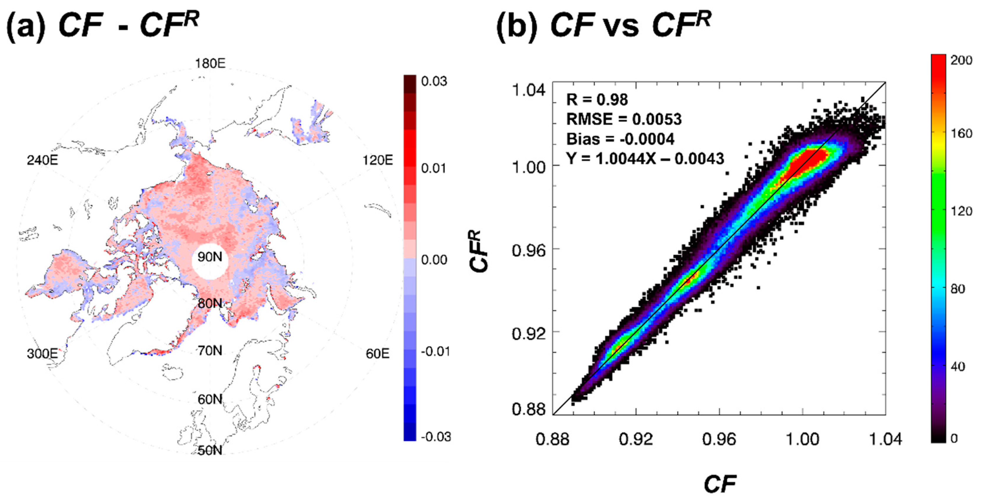
It is noted that the obtained coefficients are slightly different between polarizations, but spatial distributions and magnitudes of CFR at both polarizations are nearly identical (not shown). It is thought that the surface scattering influence on the apparent emissivity appears to be minor for sea ice in the case of the 19.4 GHz frequency, in spite of surface scattering capable of affecting the polarization state [22]. By applying the regression equation, geographical distributions of CFR are obtained for 1 January 2004 (Figure 2b), which can be compared with the AMSR-derived CF in Figure 2a. The figure shows that they are in good agreement, with small regional differences within 0.05 over the Arctic Ocean (Figure 3a). The scatterplot between CF and CFR for one month (January 2004) also clearly shows that regression-based SSM/I CFR retrievals are comparable to the direct CF, showing a correlation coefficient of 0.98. The bias and RMSE in this comparison are −0.0004 and 0.0053, respectively. In order to examine the robustness of the regression Equation (8), regressions were performed with different combinations of 8 years in the 2003–2011 period. Each year’s comparison between CF and CFR indicated that there exists a clear linear relationship between those two, with correlation coefficients above 0.97, regardless of the year given in Table 2. This suggests that the regression coefficients obtained in this study work well for other years. Because of this, we apply the coefficients in Table 1 to the whole SSM/I period.
Consequently, the results demonstrate that the CF can be predicted from Equation (8) with SSM/I TBs only. Therefore, by incorporating CFR into Equation (5), εA can be calculated by applying CF to εs. Once εA is available, it is straightforward to estimate the emitting layer temperature TE from TBsfc using Equation (2).
4. SSM/I Snow/Ice Interface Temperature (SIIT)
Since the emissivities for the smooth surface and regressed CFR values are now available for SSM/I 19.4 GHz, the apparent emissivities can be calculated from Equation (5), i.e., . The spatial distributions of regression-based apparent emissivities are given in Figure 4. The distributions are almost the same as that for the directly calculated apparent emissivity in Figure 1, demonstrating that apparent emissivity can be estimated by solely using SSM/I measurements. Because is now available for the given SSM/I measurements, the emission temperature TE can be estimated. However, because TE is in fact the temperature between snow and ice layers, as expressed in Reference [11], the obtained emission temperature is also referred to as SIIT.
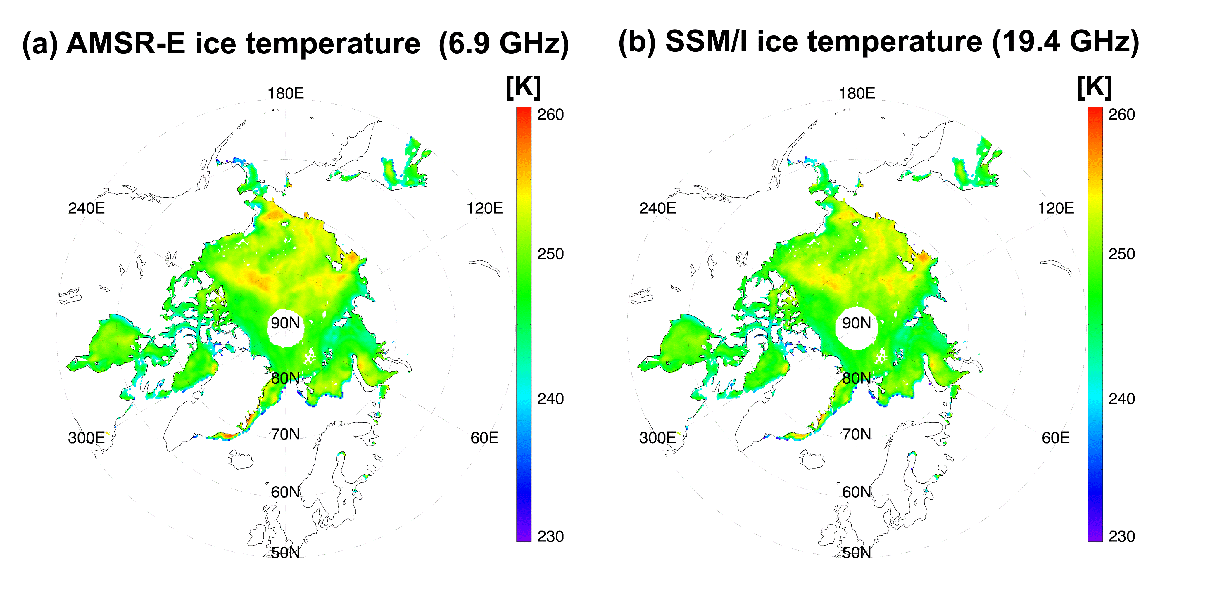
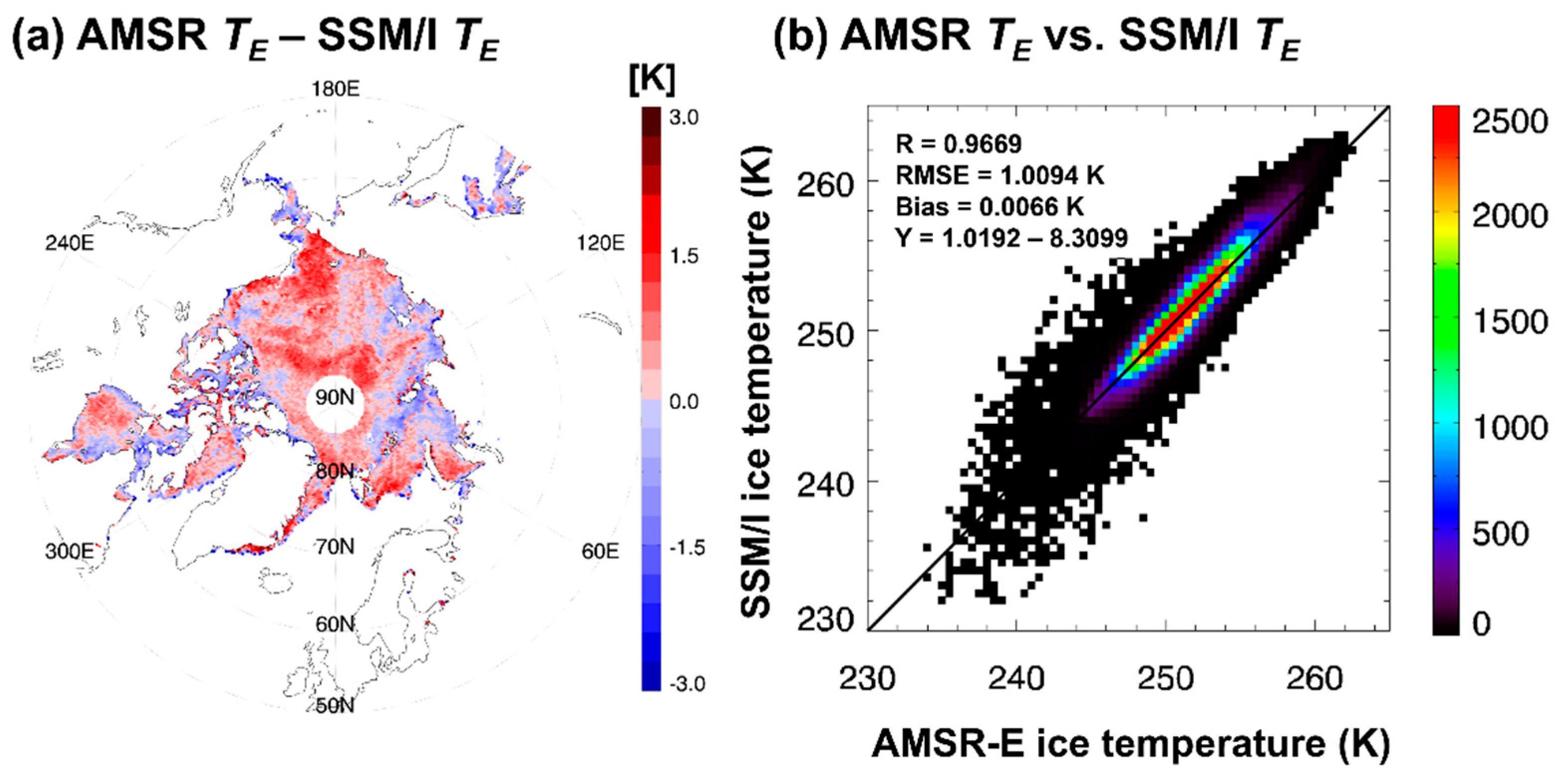
Figure 5 shows the geographical distributions of the SIIT retrieved from AMSR-E 6.9 GHz and SSM/I 19.4 GHz measurements for 1 January 2004. Note that the spatial distributions of both temperatures are similar, indicating that the retrieval method developed in this study works well for SSM/I measurements. Both distributions show relatively colder temperatures over the central Arctic Ocean and Canadian Archipelago where multiyear sea ice is prevalent. Relatively warmer temperatures are shown in the Laptev, East Siberian, and Chukchi seas, where first-year sea ice is likely present. The geographical distributions of the temperature difference between AMSR-E and SSM/I are shown in Figure 6a for 1 January 2004. The temperature difference distributions may be attributed to the difference distributions between CF and CFR because the unexplained CF variance in the regression should be propagated into the temperature difference. The two difference maps show very similar features (i.e., Figure 3a and Figure 6a). It is noted that the temperature difference is generally within 1.5 K regardless of the ice type.
A scatterplot of the temperature difference between two for January month of 2004 is provided in Figure 6b. Most of the pairs are near the one-to-one line, implying that both temperatures have a strong linear relationship. The corresponding statistics show a high correlation coefficient of 0.97 and bias (RMSE) of 0.007 K (1.01 K). It is noted that some points off the 1:1 line are in the boundary area between sea ice and open water, where water exposure often contaminates the MW measurement scene.
Validation against the Buoy Snow/Ice Interface Temperature
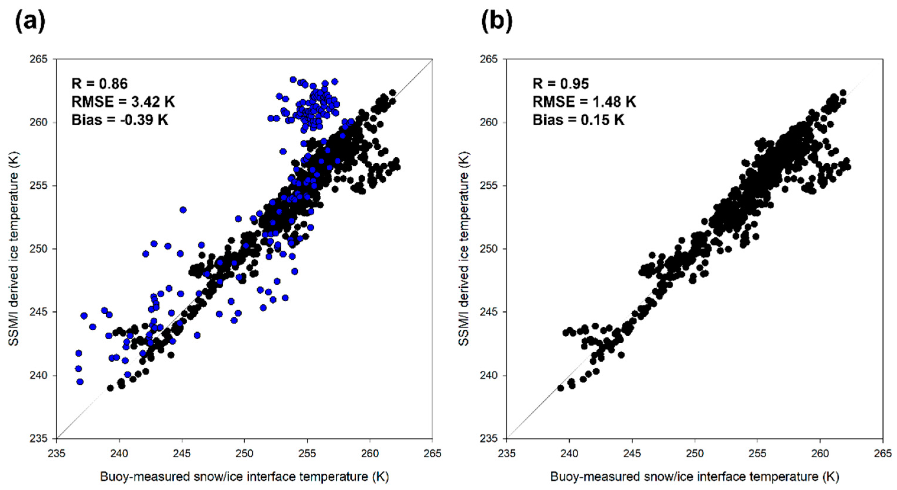
Validating the developed algorithm, retrieved SSM/I sea ice temperatures are compared with CRREL IMB drifting buoy measurements over the Arctic sea ice area [19]. For the comparison, grid-based SSM/I-retrieved temperatures are collocated with buoy data by applying the following steps: (1) Is the center point of any given SSM/I target with 25 km × 25 km resolution target located within a 12.5 km distance from the buoy location at a given time? (2) Are the corresponding sea ice concentrations greater than 98%? (3) Are the selected satellite pixels entirely covered by sea ice? (4) Select a closest target value if multiple SSM/I targets satisfy conditions (1), (2), and (3). Although the buoy data pass the above-mentioned criteria, the data are rejected if snow/ice interface information is not provided or if the data failed the quality assurance criteria given in Section 2.2. The remaining measurements along 13 deployed tracks are taken for the validation. The observation periods and start and end latitudes and longitudes are given in Table 3. Among the 13 buoy tracks, 8 were found in the northern Beaufort Sea and 5 were found in the Central Arctic Ocean, as shown in Figure S1 in the Supplementary Material.
Figure 7a shows a scatterplot of the buoy-measured SIITs and corresponding SSM/I values along all 13 buoy tracks, with a correlation coefficient of 0.86, bias of -0.36 K, and RMS error of 3.42 K. The plot shows a scattered pattern, in which the daily variation is greater than 7 K. Except for the blue dots, a large bundle of black points is located along the 1:1 line. It is noted that the scattered blue dots are associated with three buoys (#2, #6, and #8 in Table 3) in which temperature variations at the snow/ice interface are greater than 7 K for some data points. Close examination of those data reveals that such large variations are not due to the shallow ice depth or ice type (not shown). It is thought that they are likely due to problems related to the buoy instruments themselves. Rationally thinking, such large temperature variations within the ice may not be acceptable such that 7 K is subjectively applied as a criterion to remove such buoy measurements.
Because of those reasons, we exclude the blue dots in Figure 7a from the paired data set for the comparison. Comparison results obtained after applying quality assurance checks indicate a correlation coefficient of 0.95, bias of 0.15 K, and RMS error of 1.48 K (Figure 7b). It is important to note that the SSM/I-derived physical temperature of the sea ice surface shows a good 1:1 correspondence to buoy-measured SIIT, indicating that the temperature obtained for SSM/I in this study represents the temperature near the snow/ice interface defined using buoy measurements in which the typical emitting layer lay in MW frequencies.
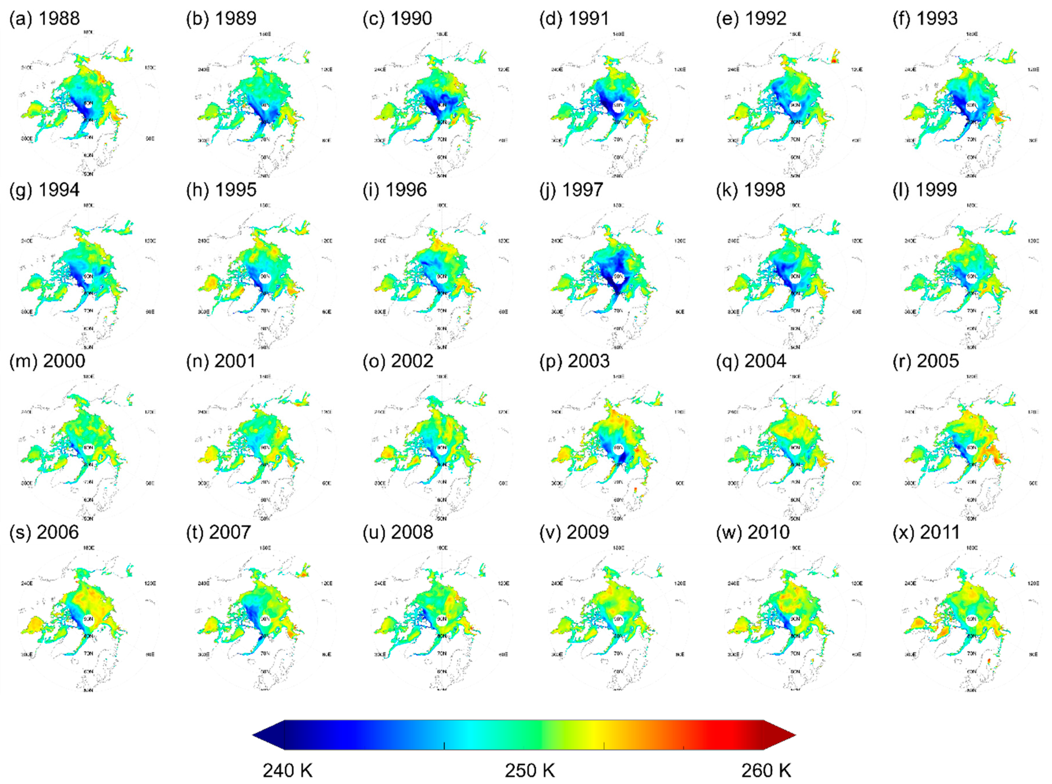
As previously discussed, we intended to produce long-term SSM/I-derived temperature information over the Arctic sea ice area. Since we developed an algorithm to retrieve the SIIT, we give an attempt to produce 24 years of SSM/I SIIT. For demonstration purposes, we generated the mean December SIIT from 1988 to 2011 and the results are given in Figure 8. The figure clearly indicates that the temperature is significantly colder in the early years of the period, suggesting that the Arctic sea ice had experienced a rapid temperature rise during the 1988–2011 period. This type of data provides important information about the evolution of climate change over the Arctic Ocean in the last decades, if we extend this effort to include the SSMIS, which effectively replaces the SSM/I.
5. Discussion and Conclusions
Aiming at producing a long-term temperature record over the Arctic sea ice area, we developed an algorithm to retrieve the wintertime SIIT over the Arctic Ocean from SSM/I FCDR data. In so doing, a simple radiative transfer model was set up, in which the snow-ice is composed of three layers (i.e., snow layer, volume scattering ice layer, and emitting ice layer, from the top). In the model, the emitting radiation from the emission layer is attenuated via volume scatterings from snow/ice layers above as well as by ice surface scattering. By using the collocated AMSR-E 6.9 GHz derived SIIT as an emission temperature for SSM/I 19.4 GHz, the apparent emissivity was determined from SSM/I 19.4 GHz TBs. The obtained apparent emissivity was then related to volume scattering and surface roughness to examine how these parameters can be related to the correction factor (i.e., the ratio between apparent emissivity at the surface and specular emissivity at the emission layer). Then the correction factor was defined and predicted from a combination of SSM/I TBs (i.e., TB19V and TB37V). The correction factor from SSM/I measurements can be used to predict the corresponding apparent emissivity from the combined Fresnel equation. It is straightforward to estimate the SIIT from SSM/I 19.4 GHz measurements once the correction factor is determined from SSM/I measurements.
The developed algorithm has been successfully implemented for SSM/I TB measurements available from July 1987. The retrieved temperatures were validated against the temperatures at the snow-ice interface (or the temperature at the top of the ice layer) from CRREL IMB drifting buoy measurements. The validation results indicated that the SSM/I-derived SIITs are in good agreement with drifting buoy measurements of the SIIT (temperature at the zero ice depth), with a correlation coefficient of 0.95, bias of 0.1 K, and RMS error of 1.48 K on a daily time scale. These results suggest that a long-term ice temperature record can be produced by applying the developed algorithm to well-calibrated long-term FCDR data composed of SSM/I and SSMIS data spanning over thirty years.
It should be mentioned that caution should be exercised if the developed algorithm is applied for thin ice because the penetration depth of the MW spectrum of interest in this study can penetrate deeper to reach the ocean water below the ice layer if the ice depth is less than approximately 16 cm, which is twice the penetration depth for first-year sea ice at 6.9 GHz with typical dielectric constant of 3.3–i0.15 [31]. In other words, a portion of the signal may be from underlying water although the magnitude is expected to be small. Additionally, the algorithm is only valid for high-concentrated sea ice pixels because the regression coefficients for the correction factor are based on TB data over the ice area with an ice concentration >98%. Therefore, when the sea ice concentration (SIC) decreases with melt ponds on the sea ice during the summer ice melt, the current approach may produce erroneous results. Furthermore, the regression coefficients for CFR may depend on the SIC products because we tried to remove possible water-contaminated pixels. We used 98% of the SIC obtained from National Snow Ice Data Center (NSIDC) product based on the National Aeronautics and Space Administration (NASA)’s bootstrap algorithm as a criterion to remove such pixels. It is known that different algorithms for the SIC (e.g., Ocean and Sea Ice Satellite Application Facility (OSI SAF), NASA Team, and Bristol algorithms among others) result in different SIC distributions with respect to seasons and regions [32,33,34,35]. However, considering that the water contamination should be largely confined within the marginal sea ice area during the winter time which we focus on in this study, the use of different data sets may provide results that do not significantly deviate from the current one. Nonetheless, it may be worthwhile to examine how different SIC data give different results, especially over the marginal sea ice area.
Supplementary Materials
The following are available online at https://www.mdpi.com/2072-4292/10/11/1795/s1, Figure S1: Tracks of the 13 selected buoys deployed in the Arctic sea. Colors indicate different buoy tracks, and numbers correspond to deployed buoys defined in Table 3. Three rejected buoys (#2, #6, and #8) are underlined in the labels.
Author Contributions
Conceptualization, S.-M.L. and B.-J.S.; Methodology, S.-M.L. and B.-J.S.; Software, S.-M.L.; Validation, S.-M.L. and B.-J.S.; Formal Analysis, S.-M.L.; Investigation, S.-M.L. and B.-J.S.; Resources, B.-J.S.; Data Curation, S.-M.L., B.-J.S., and C.D.K.; Writing-Original Draft Preparation, S.-M.L.; Writing-Review and Editing, B.-J.S. and C.D.K.; Visualization, S.-M.L.; Supervision, B.-J.S.; Project Administration, B.-J.S.; Funding Acquisition, B.-J.S.
Funding
This research was funded by the National Research Foundation of Korea (NRF) grant funded by the Korean government (MSIP) (NRF-2016R1A2B4009551).
Acknowledgments
Authors would like to thank three anonymous reviewers for their constructive and valuable comments which led to an improved paper. Authors also thank to the GCOM-W data center of Japanese Aerospace Exploration Agency (JAXA) for AMSR-E 6.9 GHz polarized brightness temperatures and NSIDC for SSM/I bootstrap sea ice concentration data.
Conflicts of Interest
The authors declare no conflict of interest.
Appendix A
Here, the method to estimate the surface roughness and volume scattering effects on the apparent emissivity is reviewed in detail. The snow-ice layer schematically simplified for the radiative transfer calculation is composed of two different layers; upper layer for volume scattering and lower layer for emission. Once MW emission occurs in the lower emission layer with emission temperature TE and corresponding rough surface emissivity (εr), the emitted TB at the surface (TBsfc), after experiencing volume scattering extinction, can be written as:
where τsca is the optical depth due to volume scatterings by snow and surface ice. Because of εr for rough surfaces, it can be expressed in terms of the smooth surface emissivity (εs) scaled by the roughness factor, F, i.e., .
Applying the roughness factor F to Equation (A1), we obtain:
By introducing the apparent emissivity (εA) concept described in Section 3.2, the following equation is obtained,
To solve Equation (A3), the smooth surface emissivity and roughness factor on the right-hand side should be parameterized in terms of basic parameters, such as the refractive index and surface roughness, using physical theory or modeling.
In the case of smooth surface emissivity, Fresnel reflection theory [30] is followed:
where εs,V and εs,H are the vertically and horizontally polarized smooth surface emissivities, respectively; Nr is the adjusted real refractive index; and θ is the satellite zenith angle. Therefore, the smooth surface emissivity can be obtained if the refractive index is known.
To parameterize the roughness effect in Equation (A3), a two-dimensional roughness model was introduced [36,37,38]. This model assumes that there are no multiple reflections on the surface and slopes of numerous rough facets that follow the Gaussian probability. There are three different factors to parameterize the rough surface emissivity: (1) locally polarized emissivity for numerous facets with different emission angles (εs,local), (2) a ratio between the area of local facets and the projected area perpendicular to the emission direction (g), and (3) an illumination function (S). Therefore, the rough surface emissivity εr can be expressed as an ensemble average of the smooth surface emissivity of numerous facets [36]:
Since the parameters of g and S are expressed as Gaussian probability density function with a root-mean-square (RMS) slope of the surface (σ), the rough surface emissivity can be calculated if Nr and σ are known. Subsequently, F can be calculated as follows:
Based on Equations (A4)–(A7), Equation (A3) can be expressed as:
Equation (A8) consists of two parts for each polarization and three unknowns (Nr, σ, and τsca). In order to solve Equation (A8), information on one of three unknowns should be ready. In this study, we employ Nr calculated in accordance with Reference [20] by assuming a spectral invariance of Nr in the MW frequencies especially for Arctic sea ice [39]. At this point, σ and τsca can be obtained from Equation (A8) if the apparent emissivity is known.
References
- Hansen, J.; Ruedy, R.; Sato, M.; Lo, K. Global surface temperature change. Rev. Geophys. 2010, 48, RG4004. [Google Scholar] [CrossRef]
- Jones, P.D.; Wigley, T.M.L. Estimation of global temperature trends: What’s important and what isn’t. Clim. Chang. 2010, 100, 59–69. [Google Scholar] [CrossRef]
- Rayner, N.A.; Parker, D.E.; Horton, E.B.; Folland, C.K.; Alexander, L.V.; Rowell, D.P.; Kent, E.C.; Kaplan, A. Global analyses of sea surface temperature, sea ice, and night marine air temperature since the late nineteenth century. J. Geophys. Res. 2003, 108, 4407. [Google Scholar] [CrossRef]
- Symon, C.; Arris, L.; Heal, B. (Eds.) Arctic Climate Impact Assessment; Cambridge Press: New York, NY, USA, 2004; p. 1042. [Google Scholar]
- Serreze, M.C.; Francis, J.A. The Arctic amplification debate. Clim. Chang. 2006, 76, 241–264. [Google Scholar] [CrossRef]
- Comiso, J.C.; Hall, D.K. Climate trends in the Arctic as observed from space. WIREs Clim. Chang. 2014, 5, 389–409. [Google Scholar] [CrossRef] [PubMed] [Green Version]
- Stroeve, J.C.; Kattsov, V.; Barrett, A.; Serreze, M.; Pavlova, T.; Holland, M.; Meier, W.N. Trends in Arctic sea ice extent from CMIP5, CMIP3 and observations. Geophys. Res. Lett. 2015, 39, L16502. [Google Scholar] [CrossRef]
- Simmonds, I. Comparing and contrasting the behavior of Arctic and Antarctic sea ice over the 35 year period 1979–2013. Ann. Glaciol. 2015, 56, 18–28. [Google Scholar] [CrossRef]
- Bintanja, R.; Selten, F.M. Future increases in Arctic precipitation linked to local evaporation and sea-ice retreat. Nature 2014, 509, 479–482. [Google Scholar] [CrossRef] [PubMed]
- Screen, J.A.; Simmonds, I. Declining summer snowfall in the Arctic: Causes, impacts and feedbacks. Clim. Dyn. 2012, 38, 2243–2256. [Google Scholar] [CrossRef] [Green Version]
- Kattsov, V.B.; Walsh, J.E. Twentieth-century trends of Arctic precipitation from observational data and a climate model simulation. J. Clim. 2012, 13, 1362–1370. [Google Scholar] [CrossRef]
- Kopec, B.G.; Feng, X.; Michel, F.A.; Posmentier, E.S. Influence of sea ice on Arctic precipitation. Proc. Natl. Acad. Sci. USA 2016, 113, 46–51. [Google Scholar] [CrossRef] [PubMed]
- Bintanja, R.; Andry, O. Toward a rain-dominated Arctic. Nat. Clim. Chang. 2017, 7, 263–267. [Google Scholar] [CrossRef]
- Cohen, J.; Screen, J.A.; Furtado, J.C.; Barlow, M.; Whittleston, D.; Coumou, D.; Francis, J.; Dethloff, K.; Entekhabi, D.; Overland, J.; et al. Recent Arctic amplification and extreme mid-latitude weather. Nat. Geosci. 2014, 7, 627–637. [Google Scholar] [CrossRef] [Green Version]
- Francis, J.A.; Vavrus, S.J. Evidence for a wavier jet stream in response to rapid Arctic warming. Environ. Res. Lett. 2015, 10, 014005. [Google Scholar] [CrossRef] [Green Version]
- Luo, D.; Xiao, Y.; Yao, Y.; Dai, A.; Simmonds, I.; Franzke, C.L.E. Impact of Ural blocking on winter warm Arctic-cold Eurasian anomalies. Part I: Blocking-induced amplification. J. Clim. 2016, 29, 3925–3947. [Google Scholar] [CrossRef]
- Liu, J.; Curry, J.A.; Wang, H.; Song, M.; Horton, R.M. Impact of declining Arctic sea ice on winter snowfall. Proc. Natl. Acad. Sci. USA 2012, 109, 4074–4079. [Google Scholar] [CrossRef] [PubMed] [Green Version]
- Kug, J.-S.; Jeong, J.-H.; Jang, Y.-S.; Kim, B.-K.; Folland, C.K.; Min, S.-K.; Son, S.-W. Two distinct influences of Arctic warming on cold winters over North America and East Asia. Nat. Geosci. 2015, 8, 759–762. [Google Scholar] [CrossRef]
- Screen, J.A. Influence of Arctic sea ice on European summer precipitation. Environ. Res. Lett. 2013, 8, 044015. [Google Scholar] [CrossRef] [Green Version]
- Lee, S.-M.; Sohn, B.-J. Retrieving the refractive index, emissivity, and surface temperature of polar sea ice from 6.9 GHz microwave measurements: A theoretical development. J. Geophys. Res. Atmos. 2015, 120, 2293–2305. [Google Scholar] [CrossRef] [Green Version]
- Berg, W.; Kroodsma, R.; Kummerow, C.D.; McKague, D.S. Fundamental climate data records of microwave brightness temperature. Remote Sens. 2018, 10, 1306. [Google Scholar] [CrossRef]
- Lee, S.-M.; Sohn, B.-J.; Shi, H. Impact of ice surface and volume scatterings on the microwave sea ice apparent emissivity. J. Geophys. Res. Atmos. 2018, 123. [Google Scholar] [CrossRef]
- Berg, W.; Sapiano, M.R.P.; Horsman, J.; Kummerow, C. Improved geolocation and earth incidence angle information for a fundamental climate data record of the SSM/I sensors. IEEE Trans. Geosci. Remote Sens. 2013, 51, 1504–1513. [Google Scholar] [CrossRef]
- Comiso, J.C. Bootstrap Sea Ice Concentration from Nimbus-7 SMMR and DMSP SSM/I-SSMIS, Version 3; NASA National Snow and Ice Data Center Distributed Active Archive Center: Boulder, CO, USA, 2017. [Google Scholar] [CrossRef]
- Polashenski, C.; Perovich, D.; Richter-Menge, J.; Elder, B. Seasonal ice mass-balance buoys: Adapting tools to the changing Arctic. Ann. Glaciol. 2011, 52, 18–26. [Google Scholar] [CrossRef]
- Comiso, J.C. Sea ice effective microwave emissivities from satellite passive microwave and infrared observations. J. Geophys. Res. 1983, 88, 7686–7704. [Google Scholar] [CrossRef]
- Masunaga, H.; Matsui, T.; Tao, W.; Hou, A.Y.; Kummerow, C.D.; Nakajima, T.; Bauer, P.; Olson, W.S.; Sekiguchi, M.; Nakajima, T.Y. Satellite Data Simulator Unit: A multisensory, multispectral satellite simulator package. Bull. Am. Meteorol. Soc. 2010, 91, 1625–1632. [Google Scholar] [CrossRef]
- Dee, D.P.; Uppala, S.M.; Simmons, J.A.; Berrisford, P.; Poli, P.; Kobayashi, S.; Andrae, U.; Balmaseda, M.A.; Balsamo, G.; Bauer, P.; et al. The ERA-interim reanalysis: Configuration and performance of the data assimilation system. Q. J. R. Meteorol. Soc. 2011, 136, 553–597. [Google Scholar] [CrossRef]
- Lee, S.-M.; Sohn, B.-J.; Kim, S.-J. Differentiating between first-year and multiyear sea ice in the Arctic using microwave-retrieved ice emissivities. J. Geophys. Res. Atmos. 2017, 122, 5097–5112. [Google Scholar] [CrossRef] [Green Version]
- Sohn, B.J.; Lee, S.-M. Analytical relationship between polarized reflectivities on the specular surface. Int. J. Remote Sens. 2013, 34, 2368–2374. [Google Scholar] [CrossRef]
- Ulaby, F.T.; Moore, R.K.; Fung, A.K. Microwave Remote Sensing: Active and Passive: Volume III: From Theory to Applications; Artech House: Norwood, MA, USA, 1986. [Google Scholar]
- Andersen, S.; Pedersen, L.T.; Heygster, G.; Tonboe, R.; Kaleschke, L. Intercomparison of passive microwave sea ice concentration retrieval over the high concentration Arctic sea ice. J. Geophys. Res. 2009, 112, C08004. [Google Scholar] [CrossRef]
- Eastwood, S.; Lavergne, T.; Tonboe, R. Algorithm Theoretical Basis Document for the OSI SAF Global Reprocessed Sea Ice Concentration Product; EUMETSAT Network Satellite Application Facilities; EUMETSAT: Darmstadt, Germany, 2014. [Google Scholar]
- Cavalieri, D.J.; Crawford, J.P.; Drinkwater, M.R.; Eppler, D.T.; Farmer, L.D.; Jentz, R.R.; Wackerman, C.C. Aircraft active and passive microwave validation of sea ice concentration from the Defense Meteorological Program Special Sensor Microwave Imager. J. Geophys. Res. 1991, 96, 21989–22008. [Google Scholar] [CrossRef]
- Ivanova, N.; Johannessen, O.M.; Pedersen, L.T.; Tonboe, R.T. Retrievals of Arctic sea ice parameters by satellite passive microwave sensors: A comparison of eleven sea ice concentration algorithms. IEEE Trans. Geosci. Remote Sens. 2014, 52, 7233–7246. [Google Scholar] [CrossRef]
- Li, H.; Pinel, N.; Bourlier, C. Polarized infrared emissivity of 2D sea surfaces with one surface reflection. Remote Sens. Environ. 2012, 124, 299–309. [Google Scholar] [CrossRef]
- Liou, K. An Introduction to Atmospheric Radiation, 2nd ed.; Academic Press: San Diego, CA, USA, 2002. [Google Scholar]
- Petty, G.W.; Katsaros, K.B. The response of the SSM/I to the marine environment. Part II: A parameterization of the effect of the sea surface slope distribution on emission and reflection. J. Atmos. Ocean. Technol. 1994, 13, 617–628. [Google Scholar]
- Warren, S.G.; Brandt, R.E. Optical constants of ice from the ultraviolet to the microwave: A revised compilation. J. Geophys. Res. 2008, 113, D14220. [Google Scholar] [CrossRef]
Figure 1.
Geographical distributions of the retrieved (a) vertically and (b) horizontally polarized apparent emissivities at 19.4 GHz of SSM/I on 1 January 2004.
Figure 1.
Geographical distributions of the retrieved (a) vertically and (b) horizontally polarized apparent emissivities at 19.4 GHz of SSM/I on 1 January 2004.

Figure 2.
Geographical distributions of (a) directly calculated CF and (b) regression-based CFR at 19.4 GHz (explained in detail in Section 3.4) on 1 January 2004.
Figure 2.
Geographical distributions of (a) directly calculated CF and (b) regression-based CFR at 19.4 GHz (explained in detail in Section 3.4) on 1 January 2004.

Figure 3.
(a) Geographical distributions of difference between CF and CFR for vertical polarization at 19.4 GHz on 1 January 2004. (b) Scatterplot between CF and CFR for January 2004. Bin sizes are 0.01 for both axes, and statistics are provided in the scatterplot.
Figure 3.
(a) Geographical distributions of difference between CF and CFR for vertical polarization at 19.4 GHz on 1 January 2004. (b) Scatterplot between CF and CFR for January 2004. Bin sizes are 0.01 for both axes, and statistics are provided in the scatterplot.

Figure 4.
Geographical distributions of the obtained apparent emissivities based on CFR for (a) vertical and (b) horizontal polarizations at 19.4 GHz on 1 January 2004.
Figure 4.
Geographical distributions of the obtained apparent emissivities based on CFR for (a) vertical and (b) horizontal polarizations at 19.4 GHz on 1 January 2004.

Figure 5.
Geographical distributions of the (a) AMSR-E 6.9 GHz and (b) SSM/I 19.4 GHz-retrieved sea ice temperature for 1 January 2004.
Figure 5.
Geographical distributions of the (a) AMSR-E 6.9 GHz and (b) SSM/I 19.4 GHz-retrieved sea ice temperature for 1 January 2004.

Figure 6.
(a) Geographical distributions of difference between AMSR-E 6.9 GHz and SSM/I 19.4 GHz-retrieved sea ice temperature for 1 January 2004. (b) Scatterplot between two temperatures for January 2004 with bin size of 0.4 K for both axes. Statistics are provided in the scatterplot.
Figure 6.
(a) Geographical distributions of difference between AMSR-E 6.9 GHz and SSM/I 19.4 GHz-retrieved sea ice temperature for 1 January 2004. (b) Scatterplot between two temperatures for January 2004 with bin size of 0.4 K for both axes. Statistics are provided in the scatterplot.

Figure 7.
(a) Scatterplots between CRREL IMB buoy-measured snow/ice interface temperature (x-axis) and SSM/I-derived temperature (y-axis), from (a) all 13 buoys, and from (b) buoys after the quality check is applied.
Figure 7.
(a) Scatterplots between CRREL IMB buoy-measured snow/ice interface temperature (x-axis) and SSM/I-derived temperature (y-axis), from (a) all 13 buoys, and from (b) buoys after the quality check is applied.

Figure 8.
(a–x) Retrieved December Arctic snow/ice interface temperature from SSM/I FCDR data from 1988 to 2011.
Figure 8.
(a–x) Retrieved December Arctic snow/ice interface temperature from SSM/I FCDR data from 1988 to 2011.


Table 1.
Regression coefficients at two polarizations in Equation (8).
| Coefficients | a0 | a1 | a2 | a3 |
|---|---|---|---|---|
| V-polarization | 0.48253852 | 0.00204367 | 0.0000556537 | −0.50878161 |
| H-polarization | 0.49223596 | 0.00201050 | −0.0000576901 | −0.52647698 |
Table 2.
Correlation coefficients between directly obtained CF and modeled CFR for each year.
| 2003 | 2004 | 2005 | 2006 | 2007 | 2008 | 2009 | 2010 | 2011 |
|---|---|---|---|---|---|---|---|---|
| 0.9811 | 0.9839 | 0.9901 | 0.9798 | 0.9859 | 0.9745 | 0.9848 | 0.9897 | 0.9777 |
Table 3.
Used data periods and starting/ending points of buoys used for validation.
| # | Period | Starting Point | Ending Point |
|---|---|---|---|
| 1 | 1 December 1993–28 February 1994 | 74.81°N, 138.55°W | 74.38°N, 154.19°W |
| 2 | 22 December 1997–28 February 1998 | 75.34°N, 150.05°W | 75.11°N, 159.66°W |
| 3 | 1 December 1997–28 February 1998 | 76.14°N, 147.46°W | 75.11°N, 159.59°W |
| 4 | 1 December 2003–29 February 2004 | 75.24°N, 135.07°W | 74.89°N, 141.07°W |
| 5 | 1 December 2006–28 February 2007 | 77.43°N, 139.35°W | 76.74°N, 139.14°W |
| 6 | 1 December 2006–2 February 2007 | 85.03°N, 128.78°E | 86.98°N, 125.96°E |
| 7 | 11 December 2007–27 February 2008 | 79.87°N, 155.15°W | 80.85°N, 151.78°W |
| 8 | 1 December 2007–28 February 2008 | 77.20°N, 135.27°W | 74.64°N, 135.14°W |
| 9 | 12 December 2007–23 February 2008 | 83.90°N, 112.91°W | 84.00°N, 109.63°W |
| 10 | 11 December 2007–28 January 2008 | 81.98°N, 119.61°W | 82.01°N, 119.76°W |
| 11 | 1 December 2008–18 February 2009 | 82.57°N, 115.30°W | 82.09°N, 114.50°W |
| 12 | 1 December 2010–28 February 2011 | 77.02°N, 149.28°W | 76.23°N, 146.66°W |
| 13 | 1 December 2010–28 February 2011 | 75.32°N, 142.39°W | 74.10°N, 142.60°W |
© 2018 by the authors. Licensee MDPI, Basel, Switzerland. This article is an open access article distributed under the terms and conditions of the Creative Commons Attribution (CC BY) license (http://creativecommons.org/licenses/by/4.0/).
Share and Cite
MDPI and ACS Style
Lee, S.-M.; Sohn, B.-J.; Kummerow, C.D. Long-Term Arctic Snow/Ice Interface Temperature from Special Sensor for Microwave Imager Measurements. Remote Sens. 2018, 10, 1795. https://doi.org/10.3390/rs10111795
AMA Style
Lee S-M, Sohn B-J, Kummerow CD. Long-Term Arctic Snow/Ice Interface Temperature from Special Sensor for Microwave Imager Measurements. Remote Sensing. 2018; 10(11):1795. https://doi.org/10.3390/rs10111795
Chicago/Turabian StyleLee, Sang-Moo, Byung-Ju Sohn, and Christian D. Kummerow. 2018. "Long-Term Arctic Snow/Ice Interface Temperature from Special Sensor for Microwave Imager Measurements" Remote Sensing 10, no. 11: 1795. https://doi.org/10.3390/rs10111795
Note that from the first issue of 2016, this journal uses article numbers instead of page numbers. See further details here.