1. Introduction
Rainfall is of primary importance in many scientific fields, such as meteorology, hydrology, agriculture, ecology and other environmental sciences [
1]. Precipitation intensity can be estimated with different techniques, including rain gauge, ground-based radar, and satellite remote sensing observations. Estimates from satellite are particularly relevant, as they assure a global coverage of the Earth [
2]. The major drawback of satellite rainfall remote sensing lies in their coarse spatial resolution, which hinders the investigation of spatial variability. This calls for the development of techniques to improve the spatial resolution of satellite rainfall remote sensing data.
A large number of downscaling methods has been developed and applied in the last few years. Most of these methods are based on the correlation between rainfall and environmental information such as latitude, longitude, altitude, slope, aspect and other orographic characteristics. In particular, Next Generation Radar (NEXRAD) daily precipitation fields were downscaled from 16 km to 4 km by considering orographic effects on precipitation distribution [
3]. This method consists of three parts, namely the rain-pixel clustering, the multivariate regression and the random cascade. In [
4], a statistical downscaling method—based on the relationships between precipitation and both terrain factors (e.g., slope, aspect and roughness) and meteorological conditions (e.g., humidity and temperature)—was proposed to disaggregate the Tropical Rainfall Measuring Mission (TRMM) 3B42 from 25 km to 1 km. Other studies introduced the positive relation between vegetation and precipitation through the use of the Normalized Difference Vegetation Index (NDVI). Among these, Ref. [
5] explored the relation between TRMM rainfall estimates and NDVI at different spatial scales; the derived relation has then been used to develop a downscaling method based on an exponential regression model. In [
6], a multiple linear regression model was developed using both NDVI and Digital Elevation Model (DEM) as independent variables. Ref. [
7] presented a geostatistical downscaling procedure, namely a geographically-weighted regression kriging, based on the relationship between precipitation and other variables, such as NDVI and DEM, to downscale the TRMM 3B43 product from 25 km to 1 km. Two methods were used in [
7]—namely a geographical difference analysis and a geographical ratio analysis—to calibrate the downscaled TRMM precipitation data. Ref. [
8] applied an integrated downscaling method, based on environmental information such as vegetation, topography, drought and albedo derived from Moderate Resolution Imaging Spectroradiometer (MODIS) products. Two different downscaling approaches—a multiple linear regression and an artificial neural network—were compared and used to downscale TRMM precipitation data from 25 km to 1 km spatial resolution. The above studies demonstrate that downscaled precipitation data better capture the spatial variability compared to the original datasets.
In this work, we downscale precipitation data derived from the operational version of the Precipitation Estimation at Microwave Frequencies (PEMW), an algorithm for surface rain intensity (SRI) retrievals, developed at the Institute of Methodologies for Environmental Analysis of the National Research Council of Italy (CNR-IMAA) [
9]. SRI data by PEMW is derived from Advanced Microwave Sounding Units (AMSU) and Microwave Humidity Sounder (MHS) radiometers on board Low-Earth-Orbit satellites and their spatial resolution range from 16 km at nadir to 51 km at maximum scanning angle. The Operative version of PEMW (OPEMW) was validated against simultaneous ground-based observations from weather radar systems and rain gauges [
10]. OPEMW SRI data are downscaled from the AMSU-B/MHS spatial resolution (16 km at the sub satellite point—SSP) to the finer MSG-SEVIRI spatial resolution (3 km at the SSP) to possibly improve their accuracy and capture higher-resolution spatial variability. Among the methods mentioned above, a kriging technique is chosen, namely kriging with external drift, as it was shown to provide estimations and associated errors with satisfactory results even in the presence of few input data. Kriging with external drift different variables and their combinations are used as auxiliary data to improve the disaggregation process. Particularly, the Brightness Temperatures (BTs) from the MSG-SEVIRI [
11] are exploited together with some environmental information, such as elevation, slope and aspect. The MSG-SEVIRI observations used here are from four channels, two centered in water vapour bands (at 6.2 µm and 7.3 µm) and two in the thermal infrared (at 10.8 µm and 8.7 µm). The precipitation episodes are divided into two types (convective and stratiform), and the trend producing the best results are searched.
The paper is organized as follows:
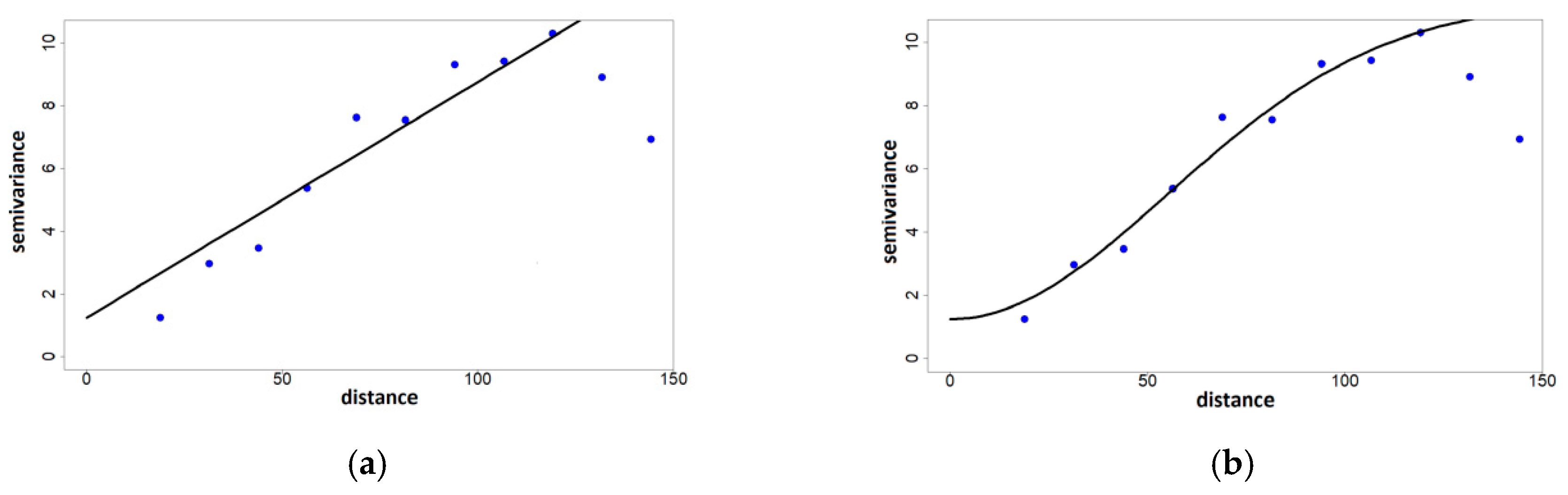
Section 2 provides a description of the data used for the implementation and the validation of the downscaling procedure; it also describes the applied methodology, focusing on the construction of the variogram and on the choice of auxiliary variables.
Section 3 shows the validation comparing downscaled surface rain rate and rain gauge measurements. In
Section 4, we draw our conclusions.
3. Results
The results of the validation are presented for the ten case studies listed in
Table 1 These cases correspond overall to 440 comparisons between observed and both original and downscaled rain data.
The continuous statistical assessment, by means of
,
RMSE,
MBE and
MAE values, is reported in
Table 2 and
Table 3 for each case and for the whole dataset, respectively. In detail, the continuous statistics show the comparison between rain gauge observations against the original OPEMW SRI data, the downscaled SRI data by ordinary kriging (OK) and the downscaled SRI data by kriging with external drift (KED), obtained using the trend producing the best results for each case.
The performances of the downscaling methods should be evaluated by considering also the original OPEMW SRI efficiency for the cases considered. The results show a reasonable improvement of the correlation coefficient in the comparison between rain gauge observations and downscaled data, compared to the original OPEMW SRI data. The agreement in terms of RMSE, MBE and MAE is better for downscaled data obtained by either of the two methods. In particular, the continuous statistics shows that kriging with external drift performs better than the ordinary kriging. In fact, the use of auxiliary information improves the estimate of the downscaled variable by +13% (corr), −37% (MBE), −8% (RMSE), and −12% (MAE). The computational cost to obtain estimates of rainfall data on the MSG-SEVIRI grid, which in our case consists of a number of pixels of 698, is about 1.2 s. Time refers to a Intel(R) Core(TM) i5-4460 CPU 3.20GHz, with 8 Gb RAM.
Among the case studies listed in
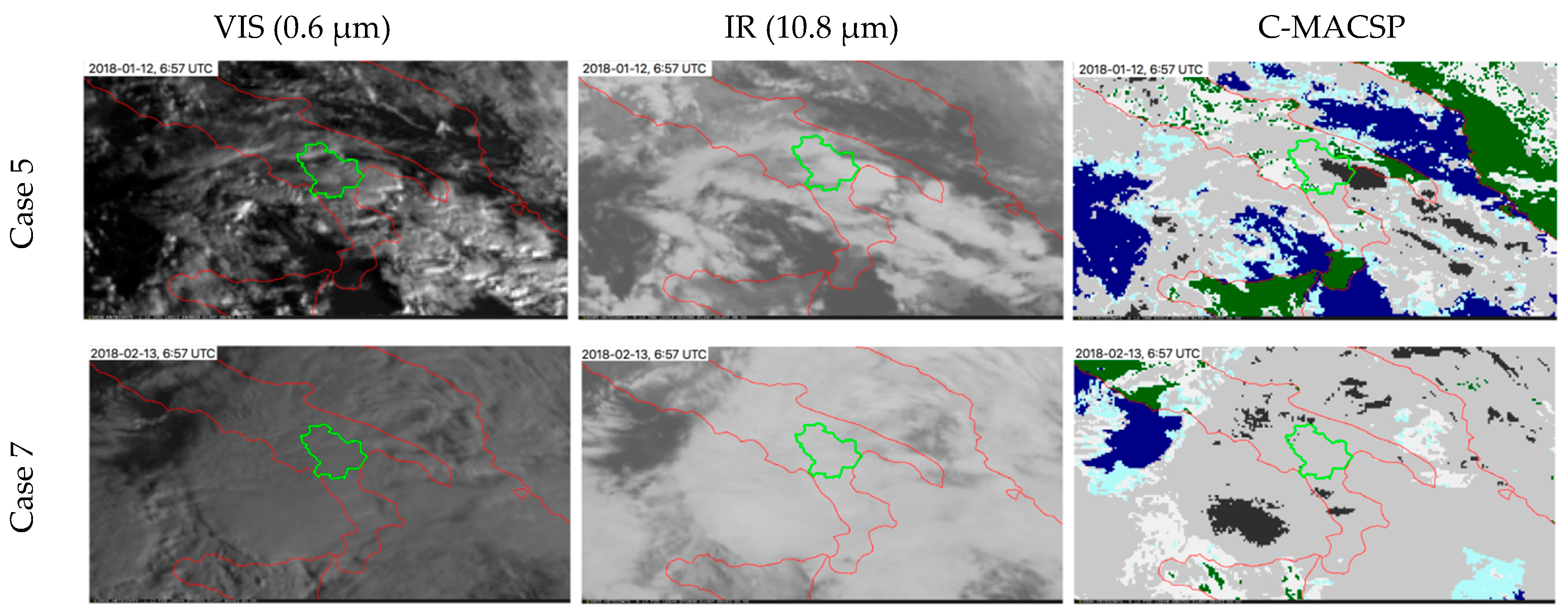
Table 1, we show in detail two representative cases (5 and 7). In
Figure 3, the MSG-SEVIRI images at VIS (0.6 µm) and IR (10.8 µm) channels and the correspondent cloud classification (C-MACSP) maps are reported for both cases. The C-MACSP maps show convection in some areas of Basilicata for case 5, while C-MACSP detects optically thick clouds in the same area for case 7. Therefore, no convection is present in the second case; however, visual inspection of the temporal sequence of MSG-SEVIRI images seem to indicate midlevel clouds—under high thick clouds detected by C-MACSP—which probably generate stratiform precipitation. The visual inspection is necessary to identify multi-layered clouds because C-MACSP does not characterize multi-layered clouds yet.
Furthermore,
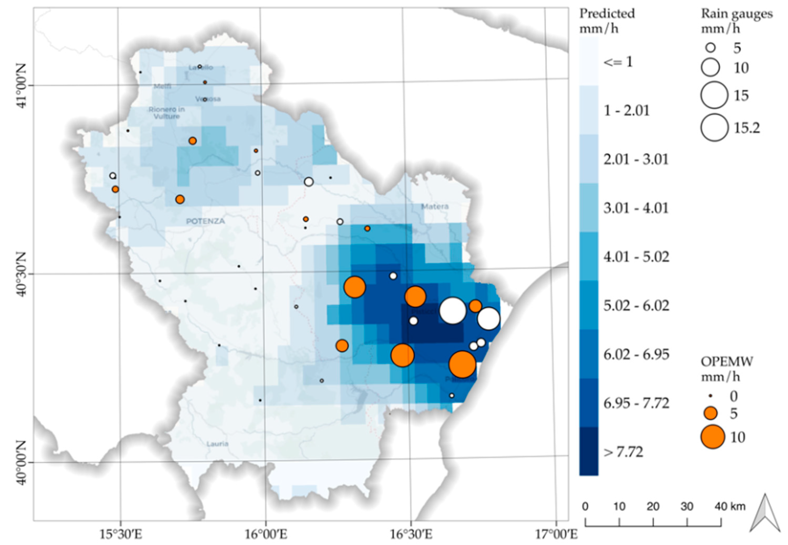
Figure 4 and
Figure 5 show the comparison between OPEMW SRI data, rain gauge observations and downscaled data by kriging with external drift. The continuous statistic for the two cases considered is reported in
Table 4 and
Table 5.
Considering case 5 (
Figure 4), the initial OPEMW SRI data set is composed by 33 pixels; out of these, only 13 feature surface rain intensity different from zero. For this case, the results show a good improvement of correlation in the comparison between rain gauge observations and downscaled data compared to the original OPEMW SRI data (0.68 against 0.48). In addition, the agreement for downscaled data in terms of
RMSE and
MAE is substantial (2.35 mm/h against 3.56 mm/h and 1.43 mm/h against 2.15 mm/h, respectively).
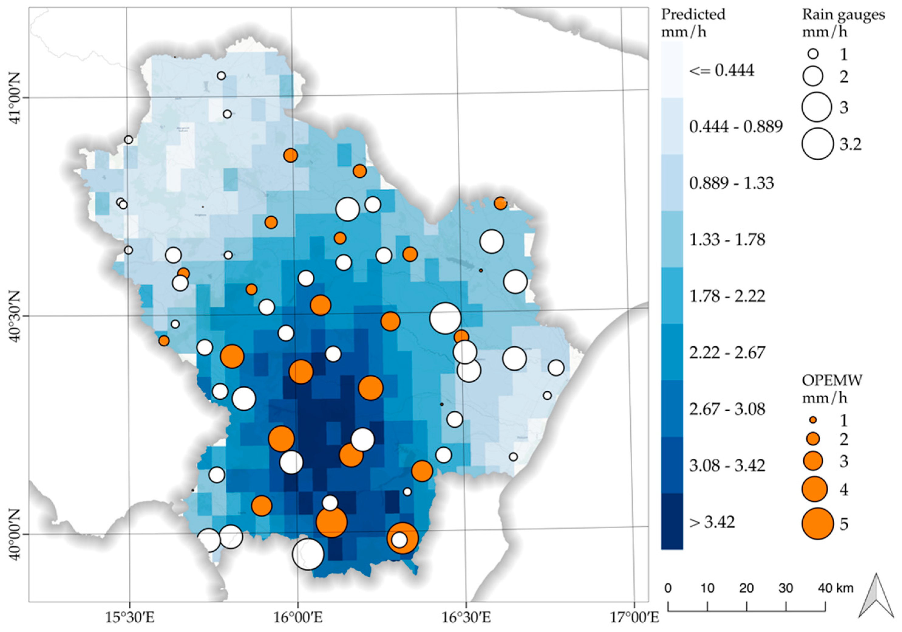
Considering case 7 (
Figure 5), the initial OPEMW SRI data set consists of 34 pixels; however, only 21 of these report surface rain intensity different from zero. In this case, the results show an improvement of correlation in the comparison between rain gauge observations and downscaled data compared to the original OPEMW SRI data (0.41 against 0.33). In addition, the agreement in terms of
RMSE and
MAE is significant for downscaled data (1.06 mm/h against 1.61 mm/h and 0.92 mm/h against 1.32 mm/h, respectively).
In both cases, the improvement obtained by using the auxiliary variables is evident.
4. Conclusions
In this paper, we have applied a geostatistical downscaling procedure, i.e., the method of kriging with external drift, in order to improve the spatial resolution of satellite-based rainfall observations from the original resolution to finer resolution. The kriging with external drift method features several additional advantages compared to standard kriging techniques, since it relies on auxiliary variables-sampled frequently and regularly [
31]—which may further minimize the error of the estimation. Therefore, a crucial step in this method lies in the selection of the auxiliary variables, which strongly depends on the parameter to be downscaled.
The known relationship between rainfall and orography [
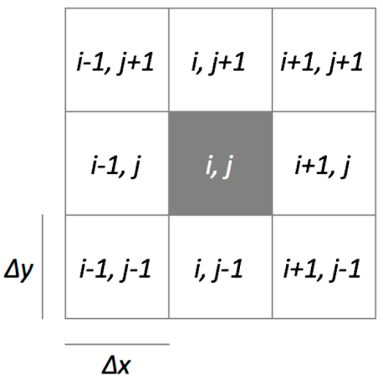
1] lead us firstly to test the slope, aspect and elevation data as auxiliary variables. Furthermore, as precipitation may generally be classified in convective and stratiform types, we also took into account the information provided by MSG-SEVIRI BT observations, acquired in the water vapor band (6.2 µm and 7.3 µm) and in thermal-IR (10.8 µm and 8.7 µm), in order to distinguish the cloud cover and precipitation types. We initially used one covariate at a time and then a combination of different covariates as external drift to find the most suitable combination yielding the best estimate for the data analysed. In detail, kriging with external drift was applied to all the proposed cases study by varying the auxiliary variables and, subsequently, analysing the validation results for each rain type separately. From this analysis, it resulted that different auxiliary variables should be used for the two rain types. In particular, we found that the trend for the convective (TREND_CR) rain cases is a combination of slope, the 8.7 µm IR channel and the difference between 10.8 μm and 7.3 μm channels, whereas, for the stratiform (TREND_SR) rain cases, the trend is a combination of the slope, the 8.7 µm IR channel and the difference between 7.3 μm and 6.2 μm channels.
To evaluate the performances of our procedure, we considered ten case studies corresponding overall to 440 comparisons between rain gauge observations and original/downscaled rain data. The statistical analysis is based on the calculation of the RMSE, MBE, MAE and correlation. The results show a reasonable improvement of the correlation coefficient in the comparison between rain gauge observations and downscaled data, compared to the original OPEMW SRI data. In addition, the agreement in terms of RMSE, MBE and MAE is better for downscaled data. In particular, the results show that kriging with external drift clearly outperforms the ordinary kriging, which only considers coordinates and distances between observations to be downscaled. In fact, the use of auxiliary information improves the estimate of the downscaled variable by +13% (corr), −37% (MBE), −8% (RMSE), and −12% (MAE). Therefore, the proposed methodology has produced results improving the statistics compared to the original OPEMW SRI data as well as the ordinary kriging. Thus, the combination of the orographic features (slope, aspect and elevation), together with MSG-SEVIRI data, represents a novelty element that allowed us to use different covariate combination for improving the quality and resolution of satellite rainfall observations.


 ,
, 


