Article

Establishment and Evaluation of a New Meteorological Observation-Based Grid Model for Estimating Zenith Wet Delay in Ground-Based Global Navigation Satellite System (GNSS)

1
School of Geodesy and Geomatics, Wuhan University, Wuhan 430079, China
2
Key Laboratory of Geospace Environment and Geodesy, Ministry of Education, Wuhan University, Wuhan 430079, China
*
Author to whom correspondence should be addressed.
Remote Sens. 2018, 10(11), 1718; https://doi.org/10.3390/rs10111718
Submission received: 8 September 2018 / Revised: 7 October 2018 / Accepted: 26 October 2018 / Published: 31 October 2018
(This article belongs to the Special Issue GPS/GNSS Contemporary Applications)

Abstract

:
With the availability to high-accuracy a priori zenith wet delay (ZWD) data, the positioning efficiency of the precise point positioning (PPP) processing can be effectively improved, including accelerating the convergence time and improving the positioning precision, in ground-based Global Navigation Satellite System (GNSS) technology. Considering the limitations existing in the state-of-the-art ZWD models, this paper established and evaluated a new in-situ meteorological observation-based grid model for estimating ZWD named GridZWD using the radiosonde data and the European Centre for Medium-Range Weather Forecasts (ECWMF) data. The results show that ZWD has a strong correlation with the meteorological parameter water vapor pressure in continental and high-latitude regions. The root of mean square error (RMS) of 24.6 mm and 36.0 mm are achievable by the GridZWD model when evaluated with the ECWMF data and the radiosonde data, respectively. An accuracy improvement of approximately 10%~30% compared with the state-of-the-art models (e.g., the Saastamoinen, Hopfield and GPT2w models) can be found for the new built model.

1. Introduction

In the precise point positioning (PPP) processing, the zenith hydrostatic delay (ZHD) is usually computed using ZHD models and meteorological data, whereas the zenith wet delay (ZWD) is estimated as a parameter in ground-based Global Navigation Satellite System (GNSS) technology [1,2]. Since the availability to high-accuracy a priori ZWD data can effectively improve PPP positioning efficiency, including accelerating the convergence time and improving the positioning precision [3,4,5], efforts have been made to build ZWD models to obtain high-precision ZWD estimates. Usually, the ZWD models can be classified into two types: the in-situ meteorological observation-based model and the empirical model. The in-situ meteorological observation-based model requires meteorological data, including the temperature, pressure or humidity, obtained from the in-situ meteorological sensors or the numerical weather prediction (NWP) model’s products as inputs. The Saastamoinen [6] and the Hopfield models [7] are widely used in-situ meteorological observation-based models. Note that the Saastamoinen-ZHD model can rather accurately estimate ZHD with measured pressure, whereas the Saastamoinen-ZWD model shows lower accuracy for the sophisticated variation of ZWD [8]. The empirical model does not depend on meteorological data and only the location (latitude, longitude and altitude) of a GNSS receiver and the specific time are required as inputs. In the early stage, the spherical harmonics function is usually employed to establish tropospheric correction models [9,10,11,12,13]. Recently, tropospheric correction models were constructed by storing model coefficients in a grid form with different spatial resolutions, which can account for both latitudinal and longitudinal variations [14,15,16,17]. The grid empirical model has been demonstrated with high accuracy and robustness, and the GPT2w model is one of the most widely used grid empirical models [18].
The coefficients of the existing in-situ meteorological observation-based models are usually globally uniform [8], rendering them insufficient to express geographic difference and reflect regional characteristics. ZWD series derived from empirical models are always “too smooth”, thus having low capability to capture the sudden changes or spike-shaped peaks emerging during the real meteorological process. In this contribution, we established and evaluated a new in-situ meteorological observation-based grid model for estimating ZWD using the radiosonde data and the European Centre for Medium-Range Weather Forecasts (ECWMF) data, in expectation to eliminate these limitations and to improve the precision of ZWD estimate. This paper is structed as follows: Section 2 describes the experimental data and the relevant methods. The establishment of the model is described in Section 3, followed by the evaluation results in Section 4. The conclusions are given in Section 5.

2. Data and Methods

2.1. Radiosonde Data

The radiosonde data derives from the radiosonde dataset of the National Climate Data Center (NCDC), which can be obtained via the Integrated Global Radiosonde Archive (IGRA). The IGRA includes high-quality observational data derived from more than 1500 radiosondes and sounding balloons from the 1960s, and users can download it for free online. The radiosonde measurements provide the temperature and humidity profiles two times each day. Since our experimental time is 2013–2016, we selected the radiosonde stations where the data for this period are available. The radiosonde stations with a lot of missing data were discarded. Eventually, in total 678 globally distributed radiosonde stations were selected, and their distribution is shown in Figure 1.

2.2. European Centre for Medium-Range Weather Forecasts (ECWMF) Data

The ECWMF dataset is a kind of NWP model’s products [19]. In this study, the ERA-Interim reanalysis of ECMWF was used for experiment. The ERA-Interim is an accurate global atmospheric reanalysis product published by ECMWF recently, which has higher quality than the previous product of ECMWF (i.e., the ERA-40 reanalysis) for higher precision and higher spatial and temporal resolutions [20]. Significant improvements have been made in the ECWMF ERA-Interim reanalysis by using the most advanced 4D-variation assimilation technologies. Besides, the ERA-Interim considers the representations of the hydrological cycle, the quality of the stratospheric circulation, and the consistency in the reanalyzed fields. The ECWMF ERA-Interim reanalysis can offer ample grid meteorological data from 1979 with the highest spatial resolution of 0.125° × 0.125° and the highest temporal resolution of 6 hours, which can be downloaded for free online. The ECMWF ERA-Interim reanalysis can provide the surface data and the pressure-level data of 37 levels from 1000 hPa to 1 hPa. In this study, the meteorological data derived from ECMWF ERA-Interim reanalysis with a spatial horizontal of 2.5° × 2.5° on a global scale at 00 UTC each day for the period of 4 years (2013–2016) were used to conduct the experiment.

2.3. ZWD Calculation Using Meteorological Data

Neither of the radiosonde measurements nor the ECMWF provides ZWD data directly, whereas the meteorological data derived from them can be used to calculate high-accuracy ZWD values. Literature [21] provided the methodology to calculate ZWD with meteorological data by directly computing the integral for wet refractive index:
ZWD = 10 6 h N w · d h = 10 6 i N w i · Δ h i
N w = k 2 · e T + k 3 · e T 2
where N w denotes the wet refractive index, i is the i th atmosphere layer, Δ h i denotes the atmosphere thickness at the i th layer (m), k 2 (16.52 K / hPa ) and k 3 (377,600 K 2 / hPa ) are the atmospheric refractive index constants [22], T denotes the atmospheric temperature (K), and e denotes the water vapor pressure (hPa).

2.4. Saastamoinen-ZWD Model

Among the in-situ meteorological observation-based models, the Saastamoinen model [6] is widely used, especially in GNSS meteorology [21,23,24,25], because it can rather accurately estimate ZHD with measured pressure. However, the Saastamoinen-derived ZWD has large uncertainty due to the high correlation between ZWD and changeable water vapor. The equation of the Saastamoinen-ZWD model is shown as:
ZWD = 0.002277 · ( 0.05 + 1255 T ) · e 1 0.00266 · cos ( 2 ϕ ) 0.00028 · h
where T and e are the temperature (K) and the water vapor pressure (hPa) at the height of the GNSS receiver, respectively, ϕ stands for the receiver latitude (radians), and h denotes the receiver height (m) above the mean sea level.

2.5. Hopfield-ZWD Model

Another widely used in-situ meteorological observation-based model is the Hopfield model [7], the ZWD calculation equation of which is shown as:
ZWD = 1.552 × 10 7 · 4810 · e · ( h w h ) T 2
where h w denotes the top height of the wet troposphere, which is approximately 11,000 m, the other parameters are the same as those in Equation (3).

2.6. GPT2w Model

The GPT2w model is a widely used empirical tropospheric correction model developed in literature [18]. The monthly mean pressure-level data of ECMWF data were used to build GPT2w, and it can provide the grid data of the mean, the annual and semi-annual parameters for a lot of meteorological elements, the equation of which is described as:
r ( t ) = A 0 + A 1 cos ( d o y 365.25 2 π ) + B 1 sin ( d o y 365.25 2 π ) + A 2 cos ( d o y 365.25 4 π ) + B 2 sin ( d o y 365.25 4 π )
where A 0 is the mean value, ( A 1 , B 1 ) represent the annual amplitude, ( A 2 , B 2 ) represent the semiannual amplitude, and d o y is the day of the year. GPT2w can provide grid parameters with spatial resolutions of 5° × 5° and 1° × 1°. The program and the GPT2w model grid coefficients can be obtained for free online. It should be noted that the GPT2w model cannot directly provide the ZWD data, the ZWD value should be calculated using the ZWD model presented in literature [23], the equation of which is shown as:
ZWD = 10 6 · ( k 2 + k 3 T m ) · R d ( λ + 1 ) · g m · e
where k 2 , k 3 and e are the same as those in Equation (3), R d (3.3776 × 10⁵ k · mb 1 ) denotes the dry air ratio gas constant, g m (9.80655 m / s 2 ) means the mean gravitational acceleration, T m represents the weighted mean temperature (K), and λ denotes the decrease factor of water vapor pressure. The values of e , T m and λ can be obtained from the GPT2w model.

3. Establishment of the Model

3.1. Correlation between ZWD and Water Vapor Pressure

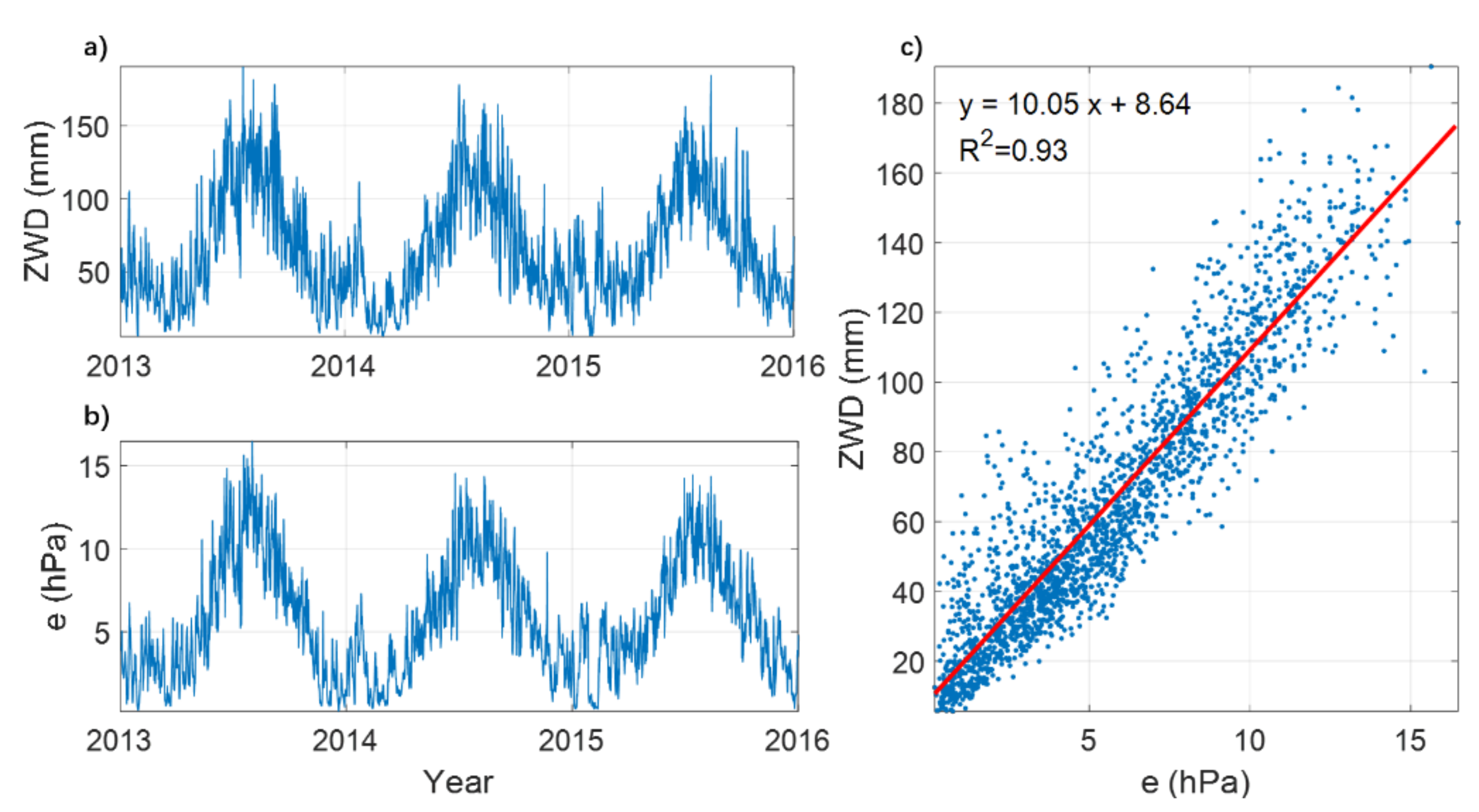
It can be found from the equations shown in Section 2 that the water vapor pressure e is a critical parameter to calculate ZWD. In this contribution, we first analyzed the correlation between ZWD and e. Figure 2a,b show the time series of ZWD and e for a 3-year period (2013–2015) at the radiosonde station 71964 (60.73°N, 135.09°W, altitude: 707 m, in Whitehorse, Canada), which legibly indicate a good agreement between ZWD and e. Figure 2c shows the linear correlation between the ZWD and e at the radiosonde station 71964. The ZWD can be very well fitted by the water vapor pressure. The correlation coefficient between them is 0.93, which indicates a rather high correlation.
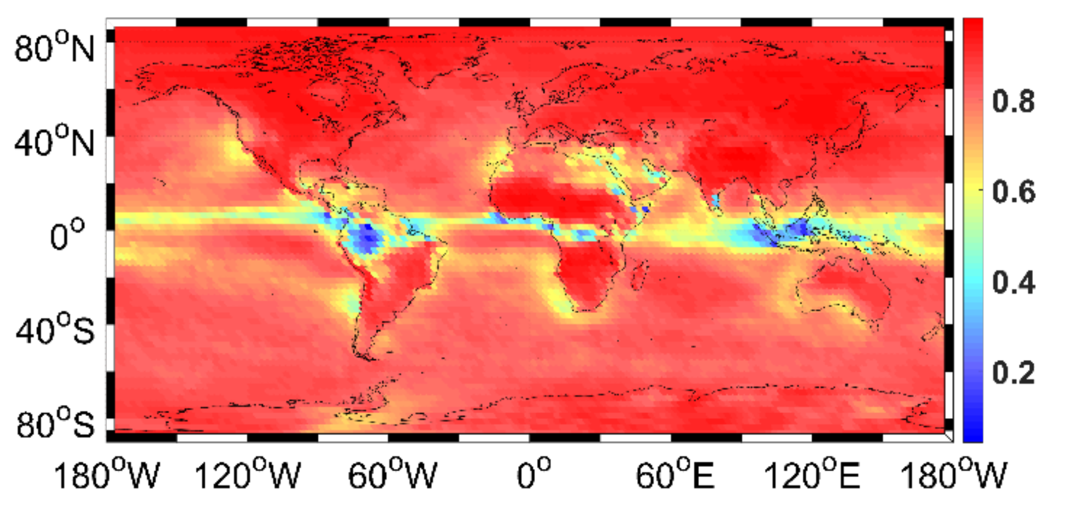
To observe the correlation between ZWD and e on a global scale, we calculated the correlation coefficients of them at each grid point with a spatial resolution of 2.5° × 2.5° using the 3-year period (2013–2015) ECMWF data, and the results are shown in Figure 3. As can be seen in Figure 3, ZWD has a strong correlation with e in most of the regions. The correlation coefficients are relatively low in tropics, whereas for the grid points at high-latitude or continental regions, the correlation coefficients are relatively large and most of the values are larger than 0.9.

3.2. Expression of the Formula and Determination of the Coefficients

According to the correlation analysis above, ZWD has a strong correlation with e, especially in high-latitude or continental regions. Thus, a linear regression ZWD model can be built by calculating the proportionality coefficient between ZWD and e. However, the correlation between ZWD and e is weak in low-latitude regions and the residuals can still be large just using the linear relationship between ZWD and e to build the model. Therefore, a nonlinear periodic function is used to model the residuals to refine the relationship. The final equations of the model are given below:
ZWD = a 0 · e + Δ ZWD
Δ ZWD = a 1 + a 2 cos ( d o y 365.25 2 π ) + a 3 sin ( d o y 365.25 2 π ) + a 4 cos ( d o y 365.25 4 π ) + a 5 sin ( d o y 365.25 4 π )
where e indicates the water vapor pressure (hPa), Δ ZWD is the ZWD residual (mm), d o y means the day of year, a 0 represents the proportionality coefficient, a 1 , a 2 , a 3 , a 4 and a 5 are coefficients of the seasonal residual correction function, a 1 denotes the mean value, ( a 1 , a 2 ) indicate the annual amplitude, and ( a 3 , a 4 ) are the semi-annual amplitude.
The grid ZWDs with a spatial resolution of 2.5° × 2.5° derived from the ECMWF data of 3 years (2013–2015) were used to determine the model coefficients with the least squares method. The model is called GridZWD. The coefficient of each grid point can exhibit the regional trait of the area around this grid point. Therefore, though the GridZWD is a global model, it can reflect regional characteristics with high accuracy and spatial resolution. Furthermore, since the new built GridZWD model has correlation with the measured water vapor pressure, it can capture the sudden changes or spike-shaped peaks in the ZWD series with better performance than the pure empirical model (e.g., the GPT2w model). The global distributions of the proportionality coefficients and the mean values of the residuals are shown in Figure 4.
As shown in Figure 4a, the proportionality coefficients are smaller in the low-latitude regions and larger in the high-latitude regions, especially in the polar regions. This may be due to the weak correlation between ZWD and e in the tropics. Additionally, the proportionality coefficients are large in some high-altitude ice-covered regions (e.g., the Qinghai-Tibetan Plateau and the Cordillera Range). Furthermore, the proportionality coefficients are large in the near-equatorial regions and in the North Sahara Desert, but are very small in some boundary areas between the oceanic and continental regions. Note that the directions of these boundary areas are similar to those of the northeast sectors (the northern hemisphere) and the southeast trades (the southern hemisphere), indicating that the distribution of the relation between ZWD and e may have correlation with thermodynamic circulation. As can be observed from Figure 4b, the mean values of the residuals are generally positive in the continental and high-latitude regions, whereas they are negative in the oceanic regions.
When we calculate ZWD at the location of a GNSS receiver, the water vapor pressure value is required, which can be obtained either from the collocated meteorological observation instruments, nearby radiosonde measurements, NWP model’s output or empirical models. Note that with the extensive distribution of the humidity sensors globally, the value of water vapor pressure can be obtained in real time in most of the regions. Thus, the GridZWD model built in this paper still has profound potential for real time application. The coefficients of four grid points closest to the GNSS receiver are used to calculate the coefficients of this location employing bilinear interpolation methodology. Then, the ZWD at the height of the water vapor pressure can be derived using Equations (7) and (8) with the obtained water vapor pressure. If the height of the water vapor pressure and the height of the GNSS receiver are different, a vertical correction is necessary to reduce the uncertainty of the derived ZWD value. The vertical correction method used in the TropGrid2 model [14] is employed, the equation of which is shown as:
ZWD = ZWD 0 · exp ( h h 0 q Z W D )
where ZWD 0 and ZWD are the zenith wet delay (mm) at the height (m) of the obtained water vapor pressure ( h 0 ) and the height (m) of the GNSS receiver ( h ), respectively, and q Z W D denotes the ZWD scale height, which is usually approximately 2000 m.

4. Evaluation Results

The evaluation results of the new built ZWD model are presented in this section. The Bias and the root of mean square error (RMS) are chosen as criteria to perform the evaluation. The equations are:
Bias = 1 n i = 1 n ( ZWD i * ZWD i )
RMS = 1 n i = 1 n ( ZWD i * ZWD i ) 2
where ZWD i * denotes the reference value, ZWD i denotes the estimated value, and n is the number of observations. The Bias reflects the deviation between the estimated and reference values, whereas RMS reflects the accuracy and robustness of a model. Note that the ZWD values have large geographic difference. These values are small (dry) in the high-latitude regions and large (moist) in the low-latitude regions [3,4]. In the moist (low-latitude) areas, the ZWD values can reach up to 300 mm, whereas in the dry (high-latitude) areas, they are sometimes smaller than 20 mm. Therefore, employing the Bias and the RMS to reveal the geographic distribution of the uncertainty of a ZWD model in a map figure is inappropriate. Considering this problem, we introduce the mean relative bias (MRB) and the relative root of mean square error (RRMS) as two additional criteria for evaluation. The equations of MRB and RRMS are presented as:
MRB = Bias 1 n i = 1 n ZWD i * × 100 %
RRMS = RMS 1 n i = 1 n ZWD i * × 100 %

4.1. Evaluation with the ECMWF Data

The ZWD series derived from the ECMWF data with a spatial resolution of 2.5° × 2.5° at 00 UTC over the whole 2016 year, which are different from those used for model establishment, were used as references. The ZWD estimates derived from two in-situ meteorological observation-based models (Saastamoinen and Hopfield), one empirical model (GPT2w) and the new built model (GridZWD) were compared with the references. The Bias, RMS, MRB and RRMS for each grid point were calculated. The global distributions of the MRBs and RRMSs of each model are shown in Figure 5.
According to the first column (MRB column) of Figure 5, the Saastamoinen model and the Hopfield model tend to have positive MRBs when estimating ZWD in the continental, high-latitude, tropical and ice-covered areas, whereas the MRBs of these two models tend to be negative in the oceanic and some land-sea boundary areas. This result indicates that the uncertainty of the in-situ meteorological observation-based ZWD model may have correlation with thermodynamic circulation, oceanic influence and glacial effect. The MRB of the GPT2w model is smaller than that of Saastamoinen and Hopfield models, but is larger than that of GridZWD model. It can be found from Figure 5b,d that the in-situ meteorological observation-based ZWD models (i.e., the Saastamoinen and Hopfield models) have large uncertainties in the ice-covered, polar, and some land-sea boundary regions. This is mainly due to the large MRB of the in-situ meteorological observation-based ZWD model in these regions. It can be observed from Figure 5f that the GPT2w model has smaller uncertainty in the low-latitude regions, whereas the RRMSs of the GPT2w model are much higher than those of the other three models in the high-latitude regions. This is due to the limitations of empirical models. Because of the influence of the oceans and the lack of a Coriolis effect, the synoptic variability in the tropics is far less than that in the other regions, whereas the high-latitude regions have large synoptic variability. Therefore, in high-latitude regions, more and larger sudden changes and spike-shaped peaks can be observed in the ZWD values during the real meteorological process. The ZWD estimates derived from the GPT2w model, which is an empirical model, are always “too smooth”, thus having low capability to capture those sudden changes or spike-shaped peaks, contributing to small MRB and large RRMS in high-latitude regions. Nevertheless, the other three models (i.e., the Saastamoinen, Hopfield and GridZWD models) are all in-situ meteorological observation-based models, where the meteorological data are required as inputs, so the ZWD values estimated from them can capture the sudden changes or spike-shaped peaks better than GPT2w model, contributing to lower RRMS. According to the statistics, the average RMSs of all the grid points of the Saastamoinen and Hopfield models are 30.6 mm and 32.2 mm, respectively. The GPT2w model has an average RMS of 33.3 mm and the GridZWD model has an average RMS of only 24.6 mm. Therefore, the accuracy improvements of approximately 19.7%, 23.7% and 26.1% are achievable by the GridZWD model when compared with the Saastamoinen, Hopfield and GPT2w models, respectively.

4.2. Evaluation with the Radiosonde Data

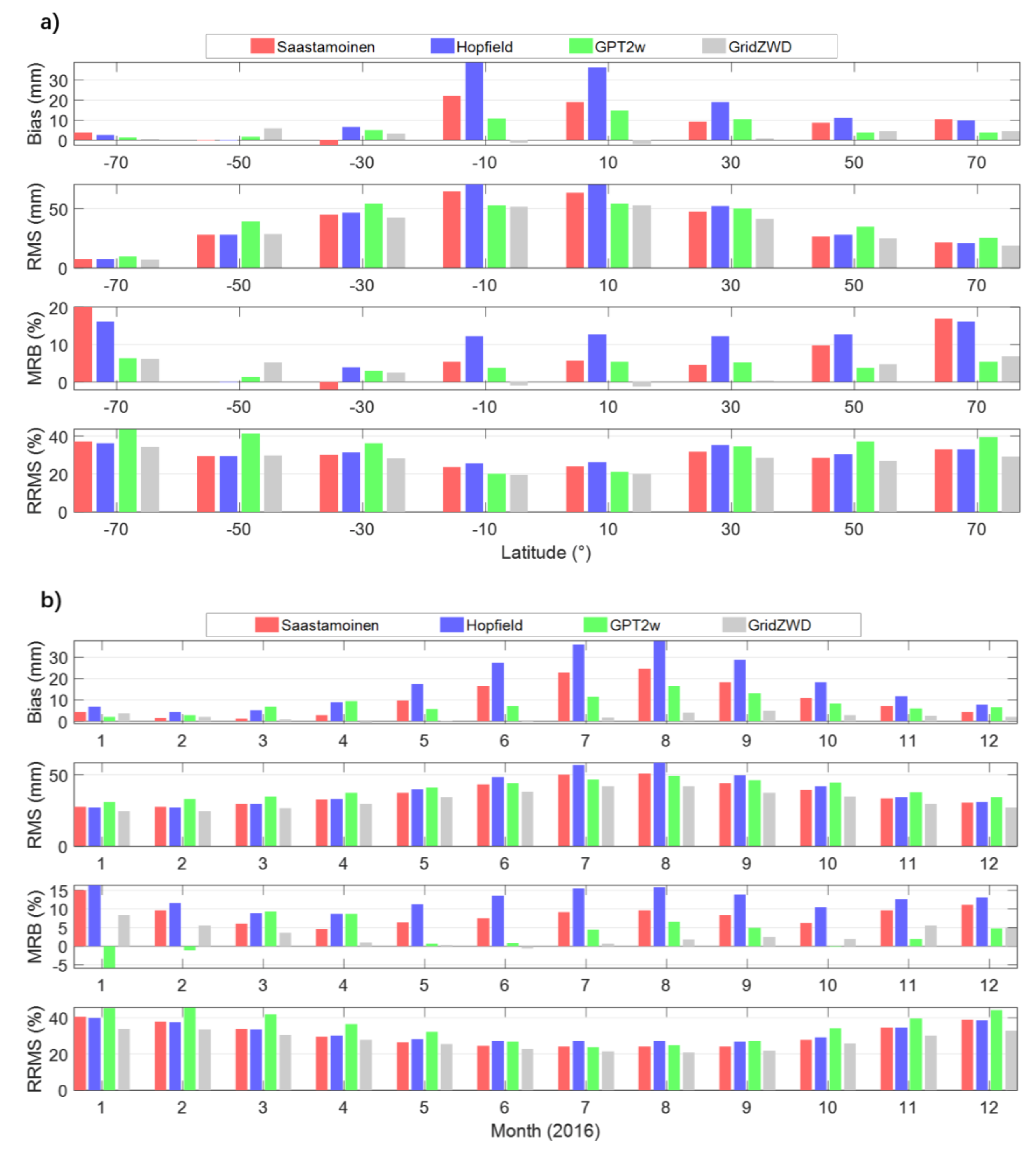
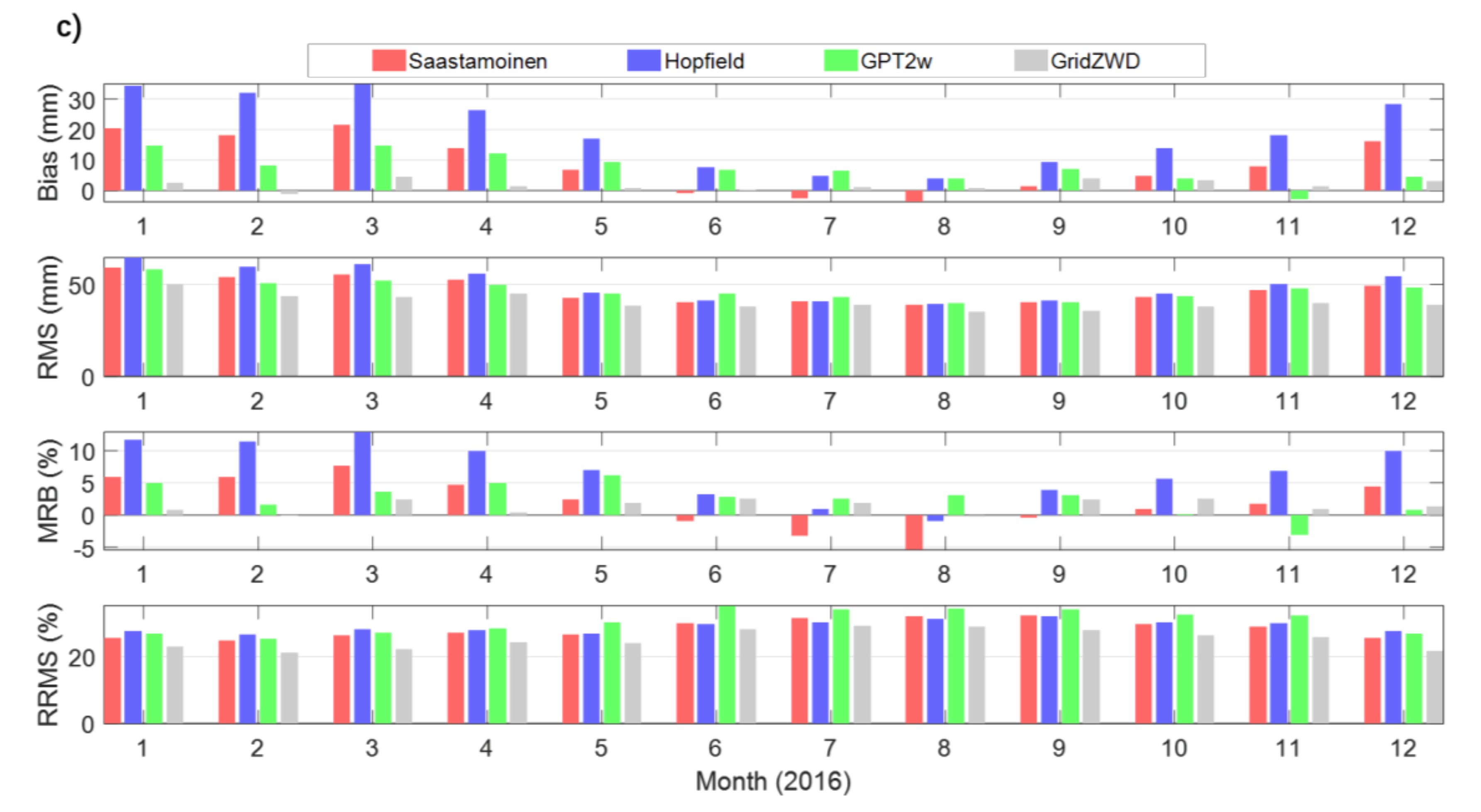
The ZWDs derived from the radiosonde measurements of the 678 stations for the 2016 year were used as independent references to evaluate the precisions of the Saastamoinen, Hopfield, GPT2w and GridZTD models. The statistical comparisons are summarized in Figure 6. The Figure 6a represents the Biases, RMSs, MRBs, and RRMSs of each model in each latitude band (20° is a latitude band), and the Figure 6b,c shows the Biases, RMSs, MRBs and RRMSs of each model in the 12 months of the 2016 year. Since the seasons of the northern hemisphere and southern hemisphere are opposite, the seasonal analysis were conducted for the two hemispheres respectively (Figure 6b for the northern hemisphere and Figure 6c for the southern hemisphere).
Figure 6 shows that the MRBs of the Saastamoinen and Hopfield models are larger than those of the GPT2w and GridZWD models and are positive. This is due to that these two in-situ meteorological observation-based models mainly have large positive MRBs in the continental areas (as is shown in Figure 5a,c), where most of the radiosonde stations are located. As can be seen from Figure 6a, the geographic distributions of the RMSs and RRMSs are different. The RMSs are larger in the low-latitude regions and smaller in the high-latitude regions, whereas the RRMSs are larger in the high-latitude regions and smaller in the low-latitude regions. The difference between the geographic distribution of RMSs and RRMSs is linked to to the increased humidity and the less synoptic variability in the low-latitude regions [3,4,8]. The GridZWD model shows smaller uncertainty than the other three models in all of the latitude bands, indicating the performance of the new built model for estimating ZWD with higher accuracy and robustness. Figure 6b,c displays the accuracies of different models in different months or seasons, from which we can find that the seasonal distributions of the RMSs and RRMSs are also different. For the northern hemisphere, which is shown in Figure 6b, the RMSs in summer are larger than those in winter, whereas the RRMSs are larger in winter and smaller in summer. This is caused by the larger quantity and smaller variability of humidity or water vapor in summer in the northern hemisphere. However, as can be observed from Figure 6c, the case of the southern hemisphere is opposite, which has smaller RMSs and larger RRMSs in summer, and has larger RMSs and smaller RRMSs in winter. For both the northern and southern hemispheres, the GridZWD model has a smaller RMS or RRMS than the Saastamoinen, Hopfield and GPT2w models during the whole 2016 year, demonstrating its superiority to the other three models. Statistics were made to calculate the average RMS of each model for all the 678 stations with the whole 2016 year. The results show that the Saastamoinen model has an average RMS of 41.3 mm, the Hopfield model has an average RMS of 44.6 mm and the GPT2w model has an average RMS of 43.6 mm. The average RMS of the GridZWD model is 36.0 mm, achieving a precision’s improvement of approximately 12.6%, 19.1% and 17.2% compared with the Saastamoinen, Hopfield and GPT2w models, respectively.

5. Conclusions

Zenith wet delay (ZWD) is usually treated as an estimated parameter in the precise point positioning (PPP) processing in ground-based Global Navigation Satellite System (GNSS) technology. Having access to high-accuracy a priori ZWD data can effectively improve PPP positioning efficiency, including accelerating the convergence time and improving the positioning precision. Thus, efforts have been made to build high-accuracy ZWD models. However, limitations can still be found in the ZWD models developed in previous studies. In this contribution, we used the radiosonde data and the European Centre for Medium-Range Weather Forecasts (ECWMF) data to investigate the relationship between ZWD and meteorological parameters. The results show that ZWD has a strong correlation with the meteorological parameter water vapor pressure e in continental and high-latitude regions and the correlation coefficients of them can reach up to 0.9 in most of the regions. Based on the analysis results, we established a new in-situ meteorological observation-based grid model called GridZWD. Another dataset of the radiosonde measurements and the ECMWF were used for evaluating the performance of the GridZWD model. The precisions of two classical in-situ meteorological observation-based models (i.e., the Saastamoinen and Hopfield models) and one state-of-the-art empirical model (i.e., the GPT2w model) were also evaluated. The results show that the Saastamoinen and Hopfield models tend to have large positive mean relative bias (MRB)s in the continental, high-latitude, tropical and ice-covered areas, but have large negative MRBs in the oceanic and some land-sea boundary areas, indicating that the uncertainty of in-situ meteorological observation-based ZWD models may have correlation with thermodynamic circulation, oceanic influence and glacial effect. The GPT2w model has large relative root mean square (RRMS)s in high-latitude regions, reflecting the limitations in empirical models. The MRBs and RRMSs of the GridZWD model are smaller than the other three models in any latitude band or in any season. When evaluated with the ECMWF data, the root of mean square error (RMS) of 24.6 mm is achievable by the GridZWD model, achieving the accuracy improvements of approximately 19.7%, 23.7% and 26.1% when compared with the Saastamoinen, Hopfield and GPT2w models, respectively. The RMS of the GridZWD model is 36.0 mm when tested with the radiosonde data with the accuracy improvements of approximately 12.6%, 19.1% and 17.2% compared with the Saastamoinen, Hopfield and GPT2w models, respectively.

Author Contributions

Data curation, Z.S.; Formal analysis, Z.S.; Funding acquisition, Y.Y.; Investigation, Z.S.; Methodology, Z.S.; Project administration, Y.Y.; Resources, C.X.; Software, Z.S.; Supervision, Y.Y. and C.X.; Validation, Z.S.; Visualization, Z.S.; Writing—original draft, Z.S.; Writing—review & editing, Y.Y. and C.X.

Funding

This research was funded by the National Natural Science Foundation of China (NNSFC), Grant Number 41574028.

Acknowledgments

The authors would like to thank ECMWF and IGRA for providing experimental data.

Conflicts of Interest

The authors declare no conflict of interest.

References

  1. Li, X.; Dick, G.; Ge, M.; Heise, S.; Wickert, J.; Bender, M. Real-time GPS sensing of atmospheric water vapor: Precise point positioning with orbit, clock, and phase delay corrections. Geophys. Res. Lett. 2014, 41, 3615–3621. [Google Scholar] [CrossRef] [Green Version]
  2. Li, X.; Zus, F.; Lu, C.; Dick, G.; Ning, T.; Ge, M.; Wickert, J.; Schuh, H. Retrieving of atmospheric parameters from multi-GNSS in real time: Validation with water vapor radiometer and numerical weather model. J. Geophys. Res. Atmos. 2015, 120, 7189–7204. [Google Scholar] [CrossRef] [Green Version]
  3. Lu, C.; Zus, F.; Heinkelmann, R.; Dick, G.; Ge, M.; Wickert, J.; Schuh, H. Tropospheric delay parameters from numerical weather models for muulti-GNSS precise positioning. Atmos. Meas. Tech. 2016, 9, 5965–5973. [Google Scholar] [CrossRef]
  4. Lu, C.; Li, X.; Zus, F.; Keinkelmann, R.; Dick, G.; Ge, M.; Wickert, J.; Schuh, H.; Wickert, J.; Schuh, H. Improving BeiDou real-time precise point positioning with numerical weather models. J. Geod. 2017, 91, 1019–1029. [Google Scholar] [CrossRef]
  5. Yao, Y.; Peng, W.; Xu, C.; Cheng, S. Enhancing real-time precise point positioning with zenith troposphere delay products and the determination of corresponding tropospheric stochastic models. Geophys. J. Int. 2017, 208, 1217–1230. [Google Scholar] [CrossRef]
  6. Saastamoinen, J. Atmospheric correction for the troposphere and stratosphere in radio ranging satellites. Geophys. Monogr. Ser. 1972, 15, 247–251. [Google Scholar]
  7. Hopfield, H.S. Tropospheric effect on electromagnetically measured range: Prediction from surface weather data. Radio Sci. 1971, 6, 357–367. [Google Scholar] [CrossRef]
  8. Zhou, C.; Peng, B.; Li, W.; Zhong, S.; Ou, J.; Chen, R.; Zhao, X. Establishment of a Site-Specific Tropospheric Model Based on Ground Meteorological Parameters over the China Region. Sensors 2017, 17, 1722. [Google Scholar] [CrossRef] [PubMed]
  9. Collins, J.P.; Langley, R.B. A Tropospheric Delay Model for the User of the Wide Area Augmentation System; Department of Geodesy and Geomatics Engineering, University of New Brunswick: Fredericton, NB, USA, 1997. [Google Scholar]
  10. Collins, J.P.; Langley, R.B. The residual tropospheric propagation delay: How bad can it get. In ION GPS; Institute of Navigation: Nashville, TN, USA, 1998. [Google Scholar]
  11. Penna, N.; Dodson, A.; Chen, W. Assessment of EGNOS tropospheric correction model. J. Navig. 2001, 54, 37–55. [Google Scholar] [CrossRef]
  12. Ueno, M.; Hoshinoo, K.; Matsunaga, K.; Kawai, M.; Nakao, H.; Langley, R.B.; Bisnath, S.B. Assessment of atmospheric delay correction models for the Japanese MSAS. In Proceedings of the 14th International Technical Meeting of the Satellite Division of The Institute of Navigation (ION GPS 2001) 2001, Salt Lake City, UT, USA, 11–14 September 2001; pp. 2341–2350. [Google Scholar]
  13. Böhm, J.; Heinkelmann, R.; Schuh, H. Short note: A global model of pressure and temperature for geodetic applications. J. Geod. 2007, 81, 679–683. [Google Scholar] [CrossRef]
  14. Schüler, T. The TropGrid2 standard tropospheric correction model. GPS Sol. 2014, 18, 123–131. [Google Scholar] [CrossRef]
  15. Lagler, K.; Schindelegger, M.; Böhm, J.; Krásná, H.; Nilsson, T. GPT2: Empirical slant delay model for radio space geodetic techniques. Geophys. Res. Lett. 2013, 40, 1069–1073. [Google Scholar] [CrossRef] [PubMed] [Green Version]
  16. Yao, Y.C.; Xu, J.; Shi, N.; Cao, B.; Yang, I.T.G. A new global GNSS tropospheric correction model. Sci. Rep. 2015, 5, 10273. [Google Scholar] [CrossRef] [PubMed]
  17. Yao, Y.; Sun, Z.; Xu, C.; Xu, X.; Kong, J. Extending a model for water vapor sounding by ground-based GNSS in the vertical direction. J. Atmosp. Solar-Terr. Phys. 2018, 179, 358–366. [Google Scholar] [CrossRef]
  18. Böhm, J.; Möller, G.; Schindelegger, M.; Pain, G.; Weber, R. Development of an improved empirical model for slant delays in then troposphere (GPT2w). GPS Sol. 2014. [Google Scholar] [CrossRef]
  19. Simmons, A.; Uppala, D.; Kobayashi, S. ERA-Interim: New ECMWF reanalysis products from 1989 onwards. ECMWF Newsl. 2007, 110, 25–35. [Google Scholar]
  20. Dee, D.; Uppala, S.; Simmons, A.; Berrisford, P.; Poli, P.; Kobayashi, S.; Andrae, U.; Balmaseda, M.; Balsamo, G.; Bauer, P. The ERA-Interim reanalysis: Configuration and performance of the data assimilation system. Q. J. R. Meteorol. Soc. 2011, 137, 553–597. [Google Scholar] [CrossRef]
  21. Bevis, M.; Businger, S.; Herring, T.A.; Rocken, C.; Anthes, R.A.; Ware, R.H. GPS meteorology: Remote sensing of atmospheric water vapor using the global positioning system. J. Geophys. Res. 1992, 97, 15787–15801. [Google Scholar] [CrossRef]
  22. Thayer, G. An improved equation for the radio refractive index of air. Radio Sci. 1974, 9, 803–807. [Google Scholar] [CrossRef]
  23. Askne, J.; Nordius, H. Estimation of Tropospheric Delay for Mircowaves from Surface Weather Data. Radio Sci. 1987, 22, 379–386. [Google Scholar] [CrossRef]
  24. Bevis, M.; Businger, S.; Chiswell, S.; Herring, T.A.; Anthes, R.A.; Rocken, C.; Ware, R.H. GPS meteorology: Mapping zenith wet delays onto precipitable water. J. Appl. Meteorol. Clim. 1994, 33, 379–386. [Google Scholar] [CrossRef]
  25. Ross, R.J.; Rosenfeld, S. Estimating mean weighted temperature of the atmosphere for Global Positioning System applications. J. Geophys. Res. 1997, 102, 719–730. [Google Scholar] [CrossRef]
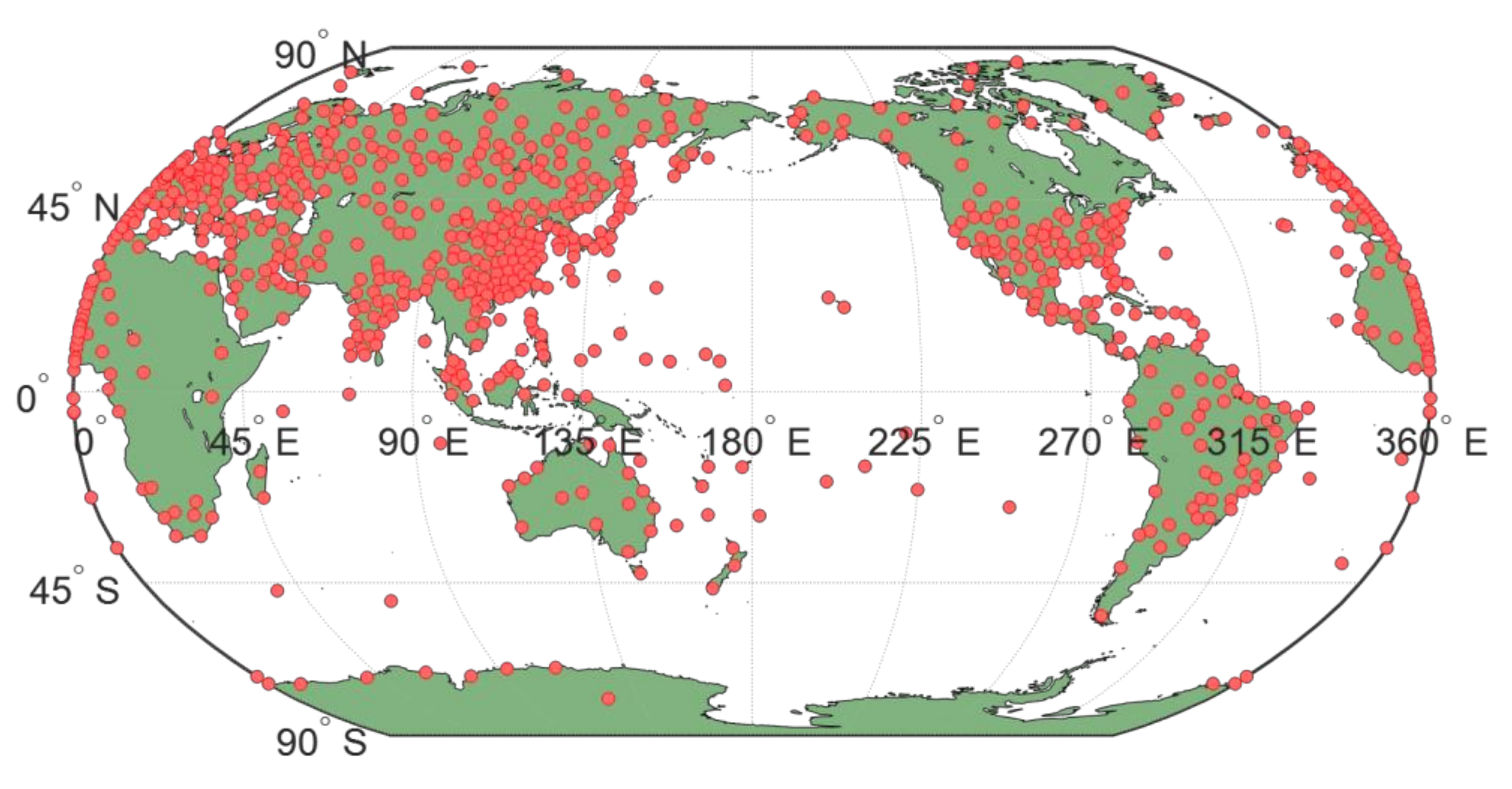
Figure 1. The distribution of the 678 selected radiosonde stations.
Remotesensing 10 01718 g001
Figure 2. Time series of zenith wet delay (ZWD) and e for a 3-year period (2013–2015) and the linear correlation between them at the radiosonde station 71964 (60.73°N, 135.09°W, altitude: 707 m, in Whitehorse, Canada). (a) 3-year time series of ZWD. (b) 3-year time series of e. (c) Linear correlation of ZWD and e. The linear regression line and the correlation coefficient are also depicted.
Remotesensing 10 01718 g002
Figure 3. The global distribution of the correlation coefficients between ZWD and e.
Remotesensing 10 01718 g003
Figure 4. The global distributions of the model coefficients calculated using the European Centre for Medium-Range Weather Forecasts (ECWMF) data for 3 years (2013–2015). (a) The global distribution of the proportionality coefficients. (b) The global distribution of the mean values of the ZWD residuals.
Remotesensing 10 01718 g004
Figure 5. The global distributions of the mean relative biases (MRBs) (first column) and relative root of mean square errors (RRMSs) (second column) of each model evaluated with the ECMWF data. (a) The global distribution of the MRBs of the Saastamoinen model. (b) The global distribution of the RRMSs of the Saastamoinen model. (c) The global distribution of the MRBs of the Hopfield model. (d) The global distribution of the RRMSs of the Hopfield model. (e) The global distribution of the MRBs of the GPT2w model. (f) The global distribution of the RRMSs of the GPT2w model. (g) The global distribution of the MRBs of the GridZWD model. (h) The global distribution of the RRMSs of the GridZWD model.
Remotesensing 10 01718 g005
Figure 6. The statistical comparisons of the radiosonde-derived ZWDs and the model-estimated ZWDs. (a) The Biases, RMSs, MRBs and RRMSs of each model in each latitude band. (b) The Biases, RMSs, MRBs and RRMSs of each model in the 12 months of the 2016 year for the northern hemisphere. (c) The Biases, RMSs, MRBs and RRMSs of each model in the 12 months of the 2016 year for the southern hemisphere.
Remotesensing 10 01718 g006aRemotesensing 10 01718 g006b