Introduction of the Double-Differenced Ambiguity Resolution into Precise Point Positioning

1
College of Surveying and Geo-Informatics, Tongji University, Shanghai 200092, China
2
School of Geodesy and Geomatics, Wuhan University, Wuhan 430079, China
3
Shanghai Geological and Mineral Engineering Investigation Co., Ltd. Shanghai 200072, China
*
Author to whom correspondence should be addressed.
Remote Sens. 2018, 10(11), 1779; https://doi.org/10.3390/rs10111779
Submission received: 5 October 2018
/
Revised: 29 October 2018
/
Accepted: 7 November 2018
/
Published: 9 November 2018
(This article belongs to the Special Issue GPS/GNSS Contemporary Applications)
Abstract
:According to the advantages of the precise point positioning (PPP) and the double-differenced (DD) model based algorithm, a new method for the integration of DD integer ambiguity resolution into PPP is presented. This method uses the undifferenced ambiguity estimated with PPP computation and the DD ambiguity generated from the DD model based algorithm to realize the PPP ambiguity fixing. In the presented method, the selection of the undifferenced ambiguity bases on the ratio test of the DD ambiguity and the ratio values based weight is used in PPP processing. This ensures the quality of the used undifferenced ambiguity. To validate the presented method, two experiments are implemented using the ten days (11 to 20 August 2014) data from local and regional reference stations and the moved two receivers. The results of the presented strategy show that improvements are achieved in all three coordinate components. The 1-h, 2-h, and 4-h PPP results indicate that the mean relative improvements were about 19%, 18%, and 15% for north, east, and up components. These results also show that prominent improvements of 29%, 31%, and 25% for north, east, and up components were obtained when the ratio values based weight was used. The application of the presented method in the displacement monitoring was implemented with the experiment and it showed that the PPP estimation computed with the presented strategy benefits local or regional displacement monitoring and improves the detecting ability for displacement.
1. Introduction
It has been more than twenty years since precise point positioning (PPP) was proposed in 1997 [1]. Precise point positioning has been demonstrated as a valuable technique for single stations positioning over continental and even global scale [2,3,4,5,6]. It has been considered as an effective tool for precise orbit determination of low Earth orbiting [7], real-time water vapor estimation [8], and determination of earthquake magnitude [9,10]. Precise point positioning can provide the coordinates with respect to a global reference frame (defined by the satellite orbits and clocks) so that its result cannot be affected by the displacement of the localized infrastructure. However the PPP ambiguities are iteratively estimated together with coordinate components, receiver clock, and tropospheric delay. The qualification that the iteration stops are based on analysis of the post-fit residual, if no more cycle slips or bad data are found. The estimated PPP ambiguity has not a natural integer feature but is the mixture of the integer ambiguity and the phase delay bias originating in the satellite and receiver. The PPP ambiguity cannot be fixed to an integer value so that the ambiguity fixing method is not used. One of the contributions of the ambiguity fixing method to the ambiguity resolution is that it provides a criterion used to assess quality of the ambiguity. There lacks assessment of the ambiguity quality in the traditional PPP. This lack is bad for the PPP positioning accuracy and convergence time. To shorten the convergence time and improve the accuracy of PPP, PPP ambiguity fixing is studied and implemented [11,12,13,14,15,16,17,18,19,20,21]. These PPP ambiguity fixing methods include: focusing on estimation of fractional cycle bias (FCB) [14,15]; improving the satellite clock products which absorb the satellite FCB [12,13,17,18]; using S-transformations, the undifferenced ambiguity of the user are fixed and resolved [19,22]. The estimation of the FCBs of the wide lane (WL) and reformed narrow lane (NL) ambiguities are usually based on the observations of the reference network and a set of complex methods [14,15,23]. In FCB estimating, it is necessary to obtain the high-quality WL and the ionosphere-free combination (IFC) ambiguities from the reference stations. Considering the time-varying characteristic of the NL FCB, the NL FCB is estimated with a step-size of 15 min [14]. For a PPP user, the products of FCBs are used to recover the integer property of PPP ambiguity. However, it still takes approximate 15~20 min to achieve the first integer ambiguity solution. In order to further shorten the PPP initialization time, the regional reference network augmented strategy was presented [8,16,23]. In these strategies, the ionosphere and troposphere delays of the PPP user are provided through interpolating the retrieved ionosphere and troposphere delays of the regional reference stations. Therefore, the estimated parameters are reduced to strengthen the geometry of the solution and realize the fast initialization of PPP positioning.
Different from these PPP strategies, all the common satellite and receiver errors are removed in the double-differenced (DD) model. The DD algorithm has the advantages of the fast convergence of the estimated parameter due to good integer characteristic of the DD ambiguity. However, the relative position (coordinate difference) is estimated and easily affected by the displacement of any one of the used receivers in DD algorithm. This limits the application of the DD algorithm, for example in earthquakes [10]. Thus, the displacement is generally monitored using the PPP results [24,25]. It is very meaningful and useful, if the advantage of the DD algorithm is used to improve the PPP ambiguity resolution (AR). Based on this consideration, a new strategy for introducing the DD integer ambiguity resolution into PPP processing is presented to obtain the high-precision PPP coordinate estimations. The introduction of the DD integer ambiguity resolution into PPP includes: (1) DD ambiguities are estimated based on the DD observations generated by the reference and user stations or two users stations; (2) undifferenced and satellite-differenced (SD) ambiguities (IFC and WL ambiguities) are generated based on WL observation and PPP computation; (3) the DD, SD IFC, and WL ambiguities are introduced in PPP. After the three steps mentioned above, the PPP ambiguity is fixed through fixing of the DD ambiguity. Using this strategy, the high-precision PPP coordinate of reference station and user or two users are obtained. In the following, the “Mathematical Models” Section introduces the method for integration of the DD integer ambiguity resolution into PPP. “Data and Experiment” and “Discussion” sections indicate the data analysis and discuss the results. Finally, the “Conclusions” Section summarizes the main findings.
2. Mathematical Models
Assuming that the residual errors of satellite orbit and clock are neglected, the SD phase ionosphere-free combination (IFC) at the user of u can be written as following:
where the superscript k and i represent tracking satellites of the user u; is the SD IFC phase observation; is the SD geometric range between receiver and satellite; is the SD IFC ambiguity and its wavelength is ; is the SD IFC satellite FCB; is the tropospheric delay; is the SD noise of phase observation. Equation (1) shows that the satellite FCB is absorbed by the SD ambiguity so that the SD ambiguity is non-integral in PPP processing. To recover the integer property of the SD PPP ambiguity, the FCB usually is estimated and used [14]. Besides the estimation method of FCB, other methods also were proposed [12,13,26,27]. Generally, the IFC ambiguity is obtained by estimating the WL and NL ambiguities. The SD phase ionosphere-free combination (IFC) for a user is also written as:
where f1 and f2 are the frequencies of L1 and L2 observations; and are SD NL and WL integer ambiguities at user u and their corresponding wavelengths are n and w. and are SD NL and WL satellite FCB; and is the light speed. Equation (2) shows that the SD PPP ambiguity still has no integer property and there are satellite biases. When a high-quality SD real-value IFC ambiguity is introduced, the SD IFC FCB can be removed and Equation (2) can be rewritten as:
where the term is the SD real-value IFC ambiguity from reference station or other user; and are DD NL and WL integer ambiguities. Equation (3) shows that the FCB is removed and a DD ambiguity is generated after a SD IFC real-value ambiguity from a reference station or other user was introduced during PPP processing. It also indicates that this DD ambiguity has a strict integer feature and it is generated from the two SD IFC real-value ambiguities. Its AR could be obtained by fixing the DD WL and NL integer ambiguities.
2.1. DD AR
Usually, the float DD ambiguity is estimated and the DD AR is fixed using the DD observations between the two observation stations. When the IFC is used, the DD AR is obtained by fixing the NL and WL AR. The SD WL ambiguity also is non-integral, since it absorbs the SD WL FCB. The SD real-value WL ambiguity could be written as:
where bwk,i is SD WL satellite FCB. Equation (4) shows that the SD WL FCB is removed and a DD WL ambiguity is generated, when a high-quality SD WL ambiguity from reference station or other user is introduced. It could be written as:
where is DD WL integer ambiguity. Equation (5) shows that the new generated WL ambiguity is actually a DD WL integer ambiguity formed with an SD WL ambiguities of a user and reference station or another user and has a good integer property. Its fixing decision for a real-value ambiguity is made by assessing its precision and closeness to an integer [28]. After the DD WL AR is obtained, the DD observation-based NL AR could be written as fowling:
2.2. PPP AR and Positioning
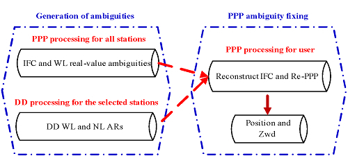
Once an SD WL and IFC ambiguities from a reference station or another user are introduced in an IFC observation and PPP computation, a new DD IFC ambiguity is generated. This new generated ambiguity is actually a difference between the ambiguities of the user and reference stations or other users and has strict integer features. The generated IFC ambiguity can be fixed by fixing the DD WL and NL AR. The generated AR can be obtained through DD observation between the user and reference stations or other users and the DD model-based algorithm. Then the rest of the parameters of position and zenith wet delay (ZWD) are resolved. The flowchart is shown in Figure 1. When the selected and generated DD and PPP ambiguities between the reference station i and user are introduced, the IFC of the user can be reconstructed as the code observations and the linearized model is written as:
where is design matrices; is the position and ZWD parameters; is the reconstructed IFC observations; and is the observation noise. For a global navigation satellite system (GNSS) network, multigroup DD ambiguities between the reference and user stations or the users are formed and generated. Thus, there are many DD ambiguities which can be selected and used for PPP AR of the user. In ambiguity fixing, the ratio test is a very popular validation test in practice [32,33]. Considering the role and significance of ratio tests in ambiguity fixing, the ratio value based weight is used. The weight function is as follows:
where is the weight of the solutions using the ambiguity of reference station i and their ratio value is . To obtain the dependable and stable estimation, the multi-reference station or other users are used and the corresponding ambiguities are generated. When n stations are used, the final parameters are estimated with weighted mean:
where is the final solutions of position and ZWD.
3. Data and Experiments
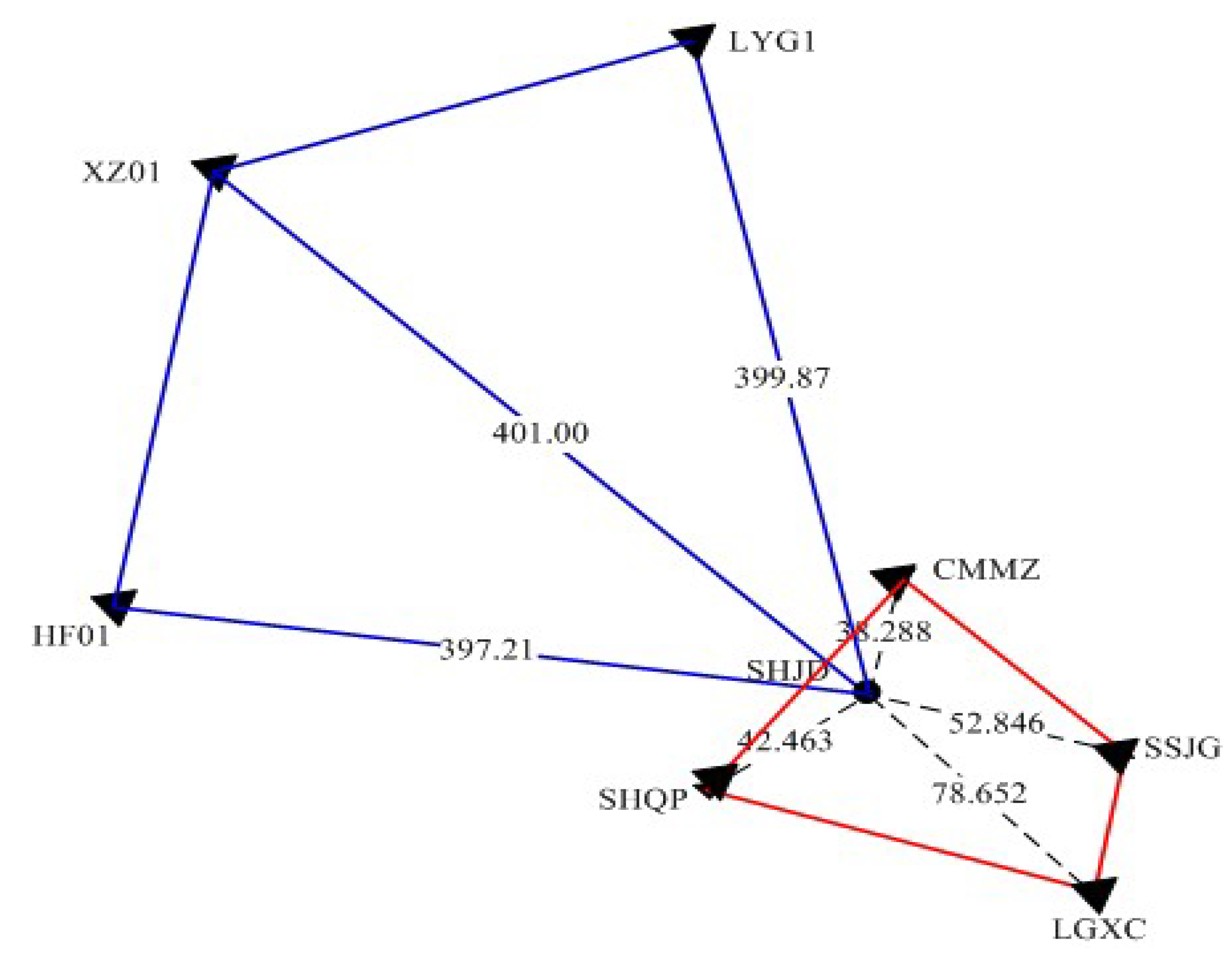
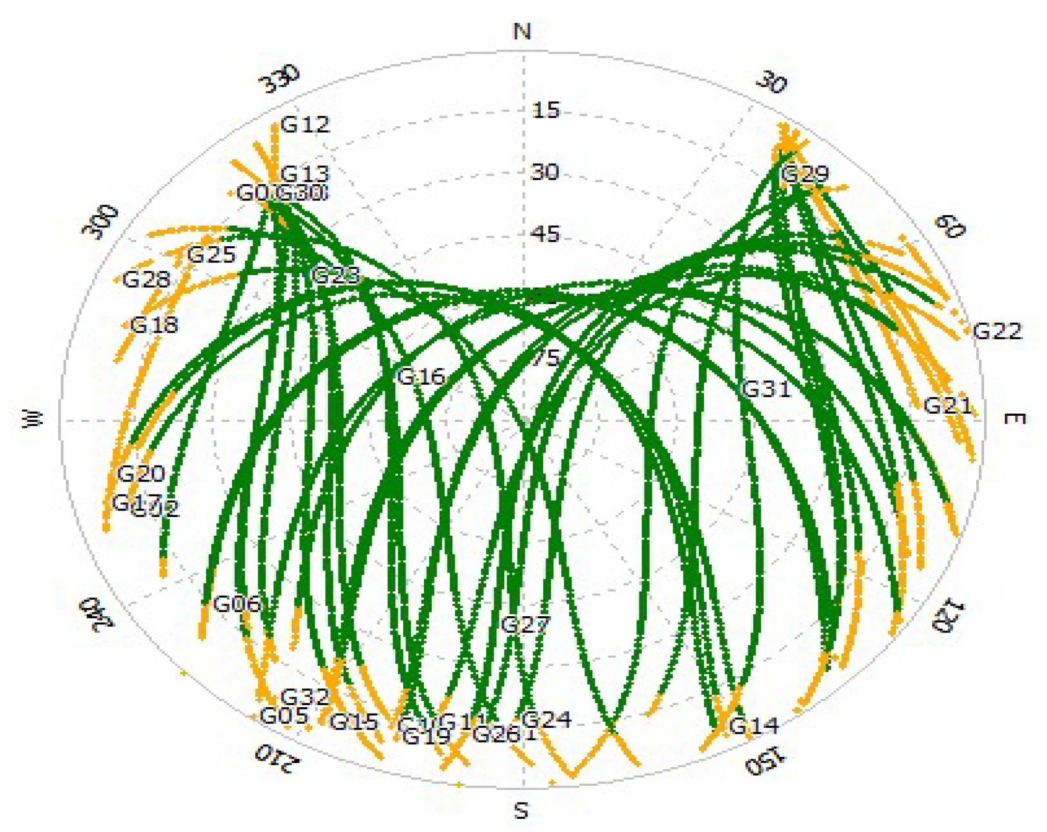
To test the presented method, two experiments were used. In the first experiment, ten days (11 to 20 August 2014) GPS data from eight stations in the Shanghai (CMMZ, SHJD, SHQP, LGXC, and SSJG) Continuous Operation Reference Station (CORS) network in Shanghai, Jiangsu (LYG1 and XZ01) and Anhui (HF01), China were used. The station SHJD was taken as a user station. Data sampling was 30 s and elevation cut-off angle was set to 9 degrees. The reference stations and user station are shown in Figure 2. The average inter-station distance of local (red) reference stations was about 53.062 km, while that of regional (blue) reference stations was about 399.36 km. Figure 3 shows the twenty-four hour skyplot of visible GPS satellites observed from Shanghai on 20 August 2014. Figure 3 indicates that there were enough observations to implement the PPP processing and validate the presented methods.
According to the presented strategy, the data from the user station was processed and the PPP coordinates were obtained in the first experiment. The DD observations between the reference stations and user were generated and the corresponding DD WL and NL ambiguities were fixed firstly. Then the SD WL ambiguities of the reference stations were computed with SD Hatch–Melbourne–Wübbena observation [34] and the corresponding SD IFC ambiguities were estimated with PPP computation. Based on the performance of the DD ambiguities, the SD IFC and WL ambiguities of reference stations and their corresponding DD WL and NL ambiguities were selected and introduced in the user PPP processing. Then the rest parameters of PPP computation just were position and ZWD and computed with the estimator of the least square. The 24-h observation at the user was split into 24 1-h, 12 2-h, and 6 4-h sessions and was processed in static mode. Three strategies #1, #2, and #3 were used to solve coordinates. No SD IFC and WL ambiguities of reference stations were used in strategy #1, while the SD IFC and WL ambiguities of reference stations and their corresponding DD ambiguities were used in strategies #2 and #3. The difference between the strategies #2 and #3 was the ratio value based weight used in strategy #3.
The second experiment was used to show the application of the presented method in the displacement monitoring of the reference station. The advantage of PPP computation is that the position with respect to a global reference frame is obtained and the estimated position cannot be affected by the shift of the localized infrastructure. This feature also shows that the displacement monitoring of the observation station can be realized based on its own observation. To evaluate the performance of the integration of the DD integer ambiguity resolution into PPP computation and analyze the potential advantage of the presented method, the second experiment was carried out on 12 August 2014. In this experiment, two GNSS receivers were used and the 12-h data was collected. The difference between the first 6-h and second 6-h observations was that the relative position of the two receivers remained unchanged, although the two receivers were moved. The inter-station distance was about 300 m. Data sampling was 30 s.
In both experiments, the final International GNSS Service (IGS) [35,36] products of the satellite clock and orbit were used. The elevation-dependent function was used:
where θj is the satellite elevation at epoch j. The corrections for the Earth rotation, Earth tides, relativistic effects, phase center variation (PCV), and differential code bias (DCB) are implemented [37]. The tropospheric delay was corrected using the Saastamoinen model and the rest wet part was estimated by setting up a piece wise constant (PWC) at an interval of 1 h. The settings for the PPP processing are shown in Table 1.
4. Discussion
In this section, the PPP solutions estimated with different strategies are analyzed first. After that, the results of the different methods in the displacement monitoring are used to validate the advantage of the presented method.
4.1. PPP Solutions
The PPP computation is implemented according to the strategies #1, #2, and #3. The ten days (11 to 20 August 2014) PPP results of strategies #1, #2 and #3 for 1-h sessions with respect to the ground truth coordinates for three coordinate components of north, east, and up are computed and illustrated in Figure 4. The ground truth coordinates were obtained using GAMIT software and the IGS station of SHAO is fixed in processing. From Figure 4, it is observed that obvious improvement was obtained when the strategies #2 and #3 were used. These results demonstrate the PPP ambiguity fixing was beneficial for improving the accuracy of the PPP positioning. The results using local reference stations estimated with the three strategies of the first 1-h session are illustrated in Figure 5. Figure 5 shows that the convergence times of strategies #2 and #3 were slightly better than that of strategy #1. The mean convergence times for different strategies and sessions were analyzed. The mean convergence times of strategies #1, #2, and #3 are 13, 10, and 10 min, respectively. The convergence time results also verify that the presented method is effective.
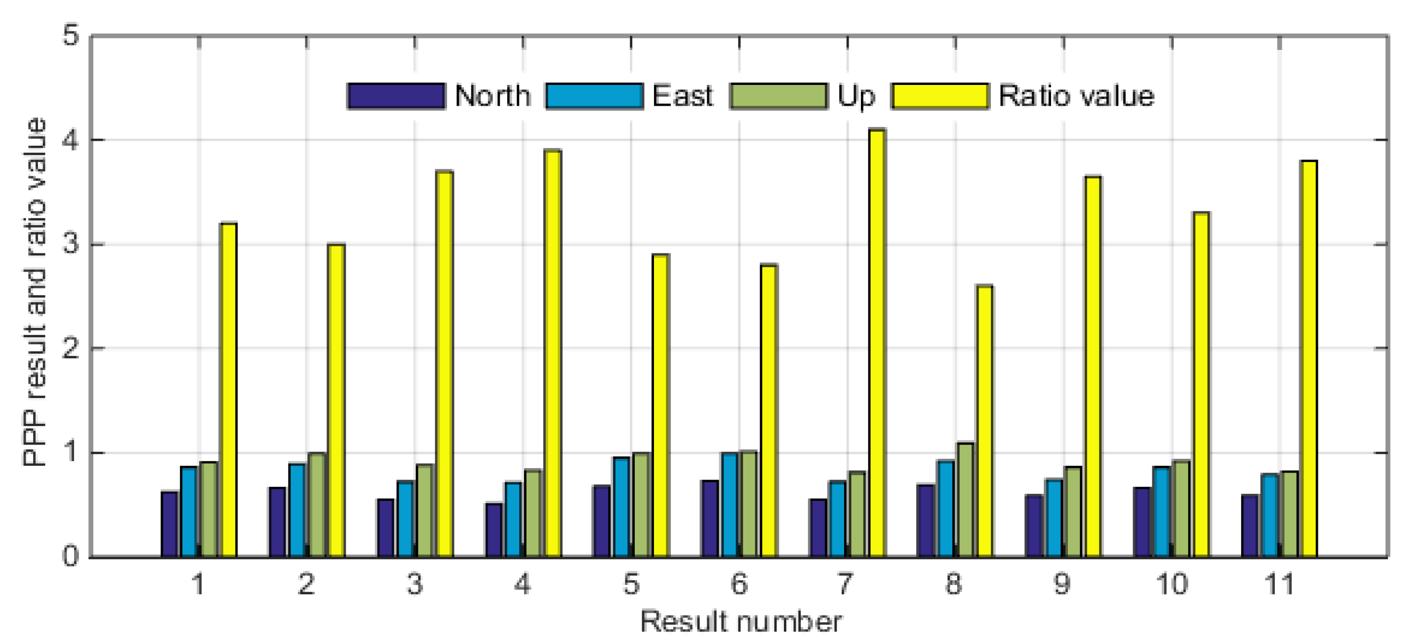
The performances of the convergence times and the positioning results verify the validity of the presented method. To analyze application of the ratio value based weight in PPP computation, the PPP results for the different ratio values are compared. The PPP results for three coordinate components of north, east, and up for 4-h sessions and the ratio values of different DD processing are illustrated in Figure 6. Figure 6 indicates that the accuracy of the PPP result improves with the ratio values of the selected DD ambiguity processing. This validates that the PPP results are related to the quality of the selected and used ambiguities of other users or stations and also advises that the high-quality should be selected to realize PPP ambiguity fixing and improve the PPP results, when the presented methods are used.
The PPP solution RMSs of different sessions for the three coordinate components of north, east, and up are shown in Table 2 and Table 3. From Table 2 and Table 3, it can be seen that improvements were achieved in all three coordinate components when the presented strategies were used. The results of the local reference in Table 2 show that the mean relative improvements were about 20%, 18%, and 15% for north, east, and up components, when the data was processed with strategy #2. When the ratio test and the ratio value based weight were used, the improvements of the local reference were obvious and the improvements reached 28%, 30%, and 25% for the north, east, and up components. The improvements further validate that the presented strategy benefits the improvement of the PPP computation accuracy. Comparing the results of the local and regional reference stations, their improvements were almost equal. This demonstrates that the PPP performances are not affected by the distance between the user and the used reference station.
In order to validate the presented methods and analyze the solutions, the baseline solutions between the user and reference stations are computed using the PPP estimations. The baseline solution RMSs with respect to the truth coordinates estimated with DD observation are computed for three coordinate components of north, east, and up and shown in Table 4 and Table 5. The results show that the accuracy of the baseline solutions can be improved, when the PPP ambiguity fixing is considered. The mean relative improvements are about 6%, 6%, and 11% for the north, east, and up components. The baseline solutions also indicate that improvements can be obtained when the ratio value based weight is used. The results of local and regional reference stations show that the baseline solutions generated from PPP results are not subject to the distance between the user and reference stations. Comparing the baseline solutions generated from the PPP solutions and the DD model based method, it is noticed that there is the difference between the two sets of baseline solutions. The difference can be explained that there are residual space-correlation errors, such as the ionospheric delay, which affects the PPP solutions and this effect cannot be removed by the coordinate-differenced algorithm. The correlation coefficient is used to validate this explanation. The correlation coefficients of the residuals from different stations for PPP computation are computed as:
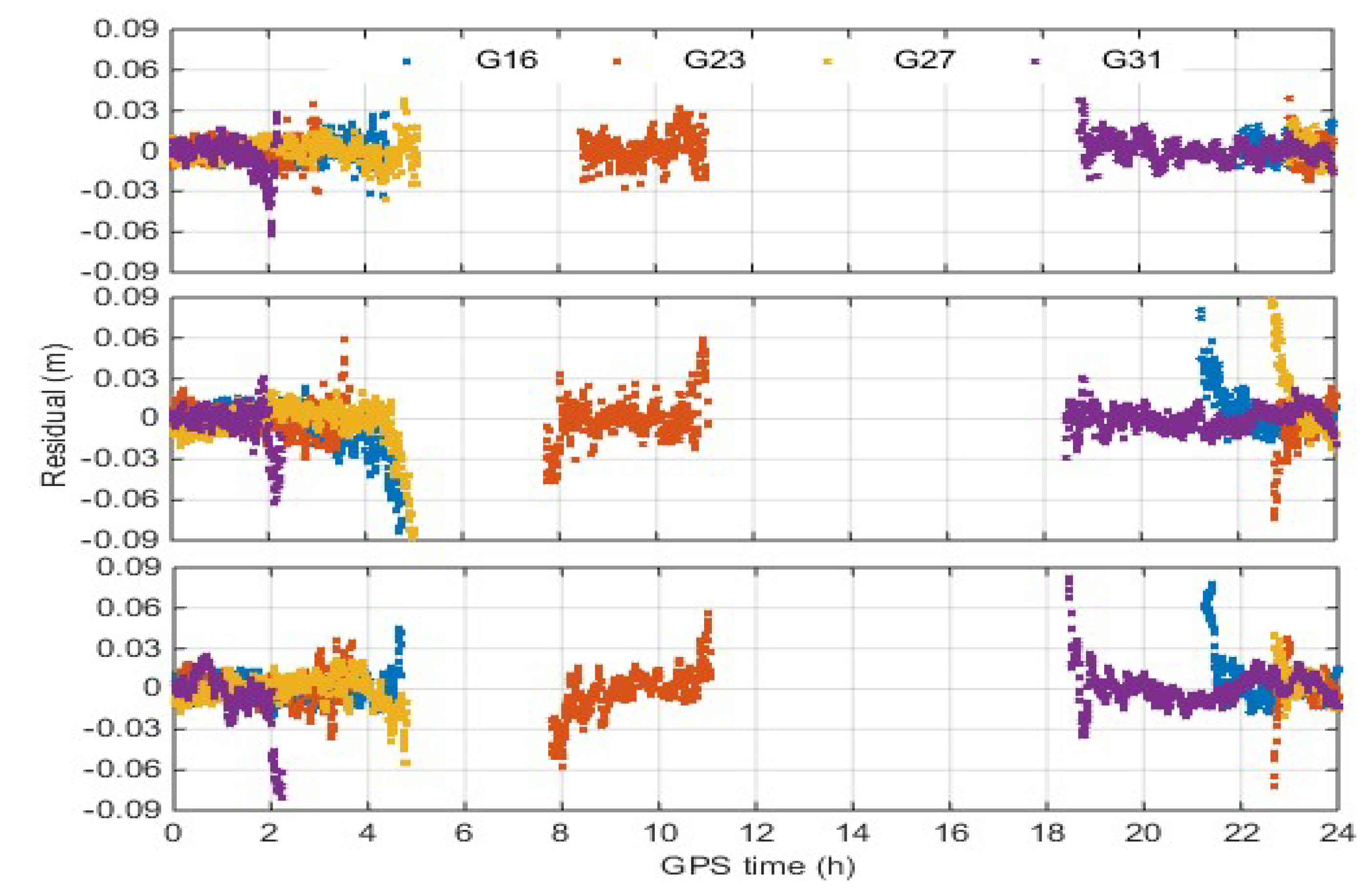
where is the covariance of the residuals for the PPP computation from two stations of i and j; is variance of the PPP residuals from the station i and is the variance of the PPP residuals from the station j. The residuals of the phase observations form the user station of SHJD and the reference stations of CMMZ and LGXC for the PPP computation are shown in Figure 7. Figure 7 show that the residuals from the three stations have the similar trends. The similar trends demonstrate that there are some space-correlation errors, which cannot be modeled and affect the PPP accuracy. The mean value of the correlation coefficients is bigger than 0.3 and the values can validate the above interpretation. To further improve the accuracy of the PPP computation and obtain the equivalent results of DD model, these un-modeled errors should be considered and corrected. But, this is beyond our scope in this study.
4.2. Application in Displacement Monitoring of the Reference Station
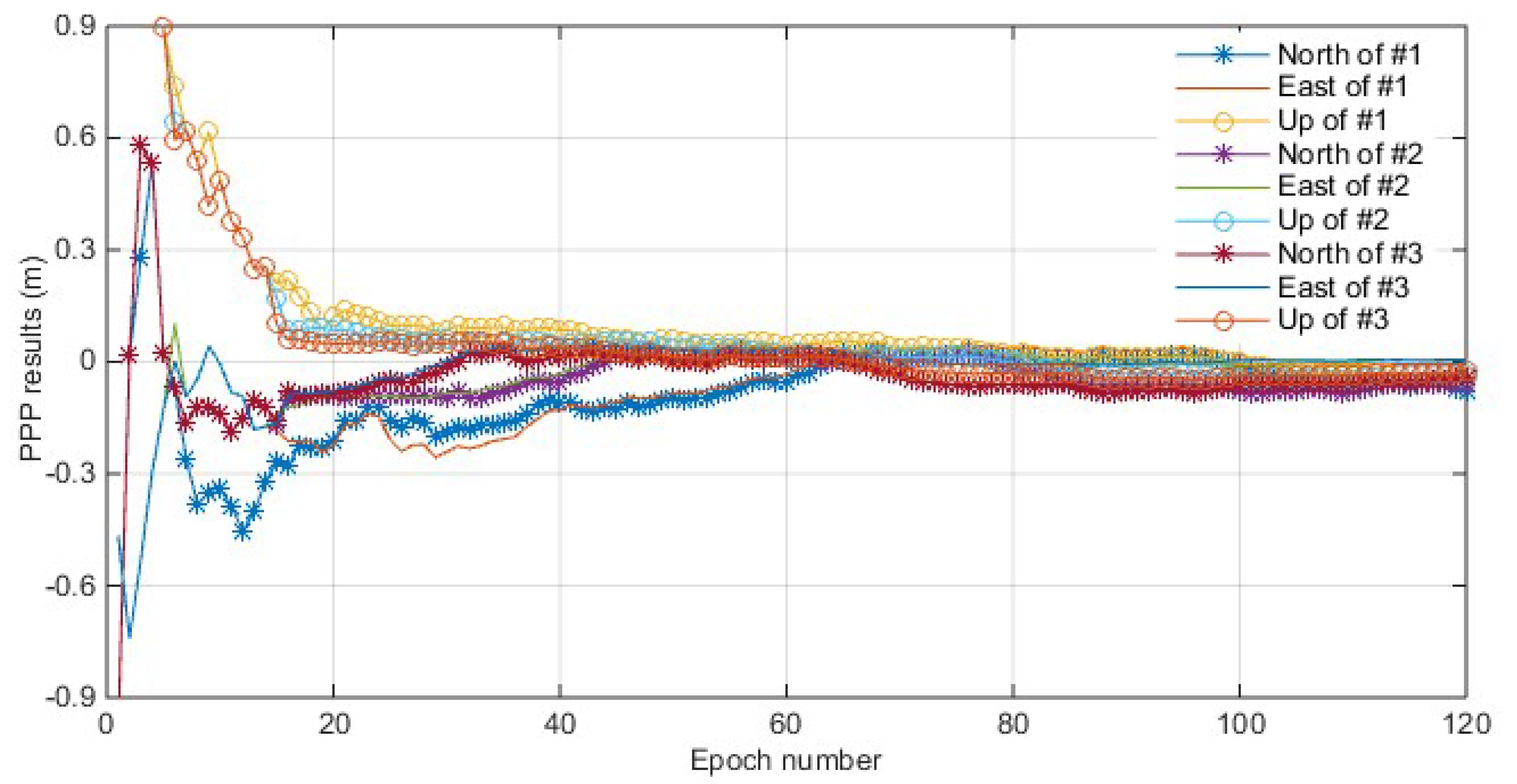
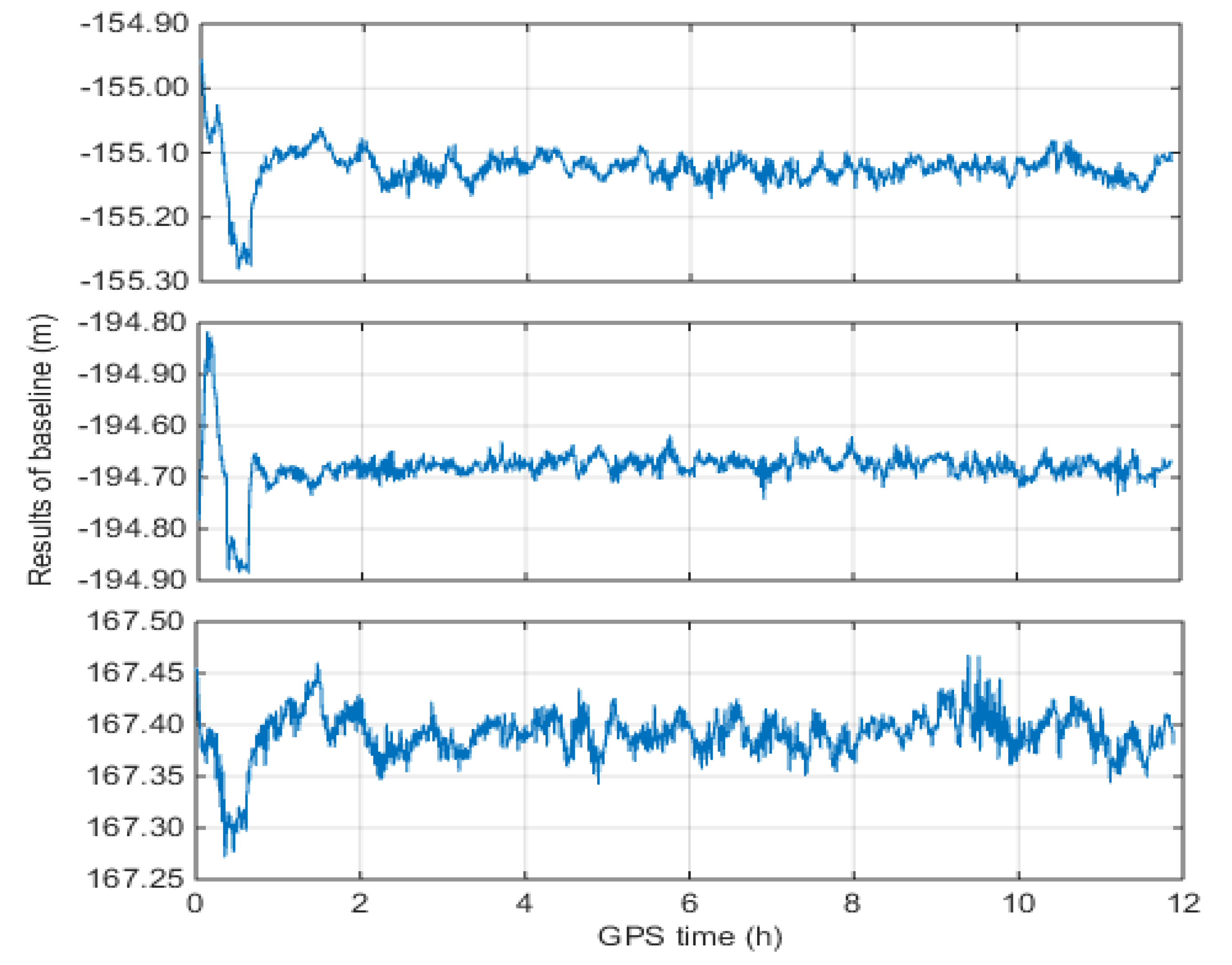
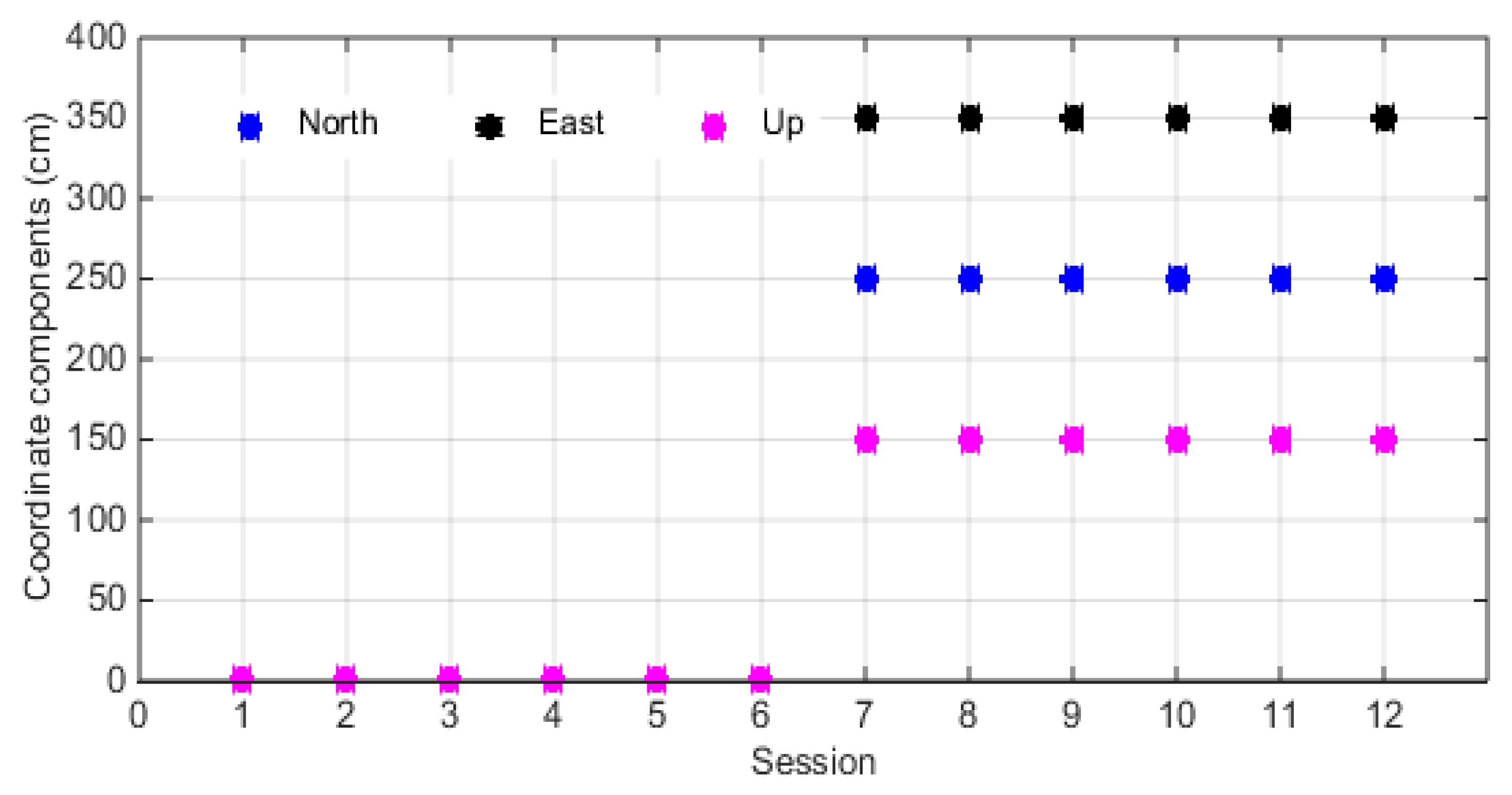
The 12-h data of the second experiment is processed with PPP computation, in which the ambiguity is fixed using the presented strategy. It also is processed with DD algorithm. The results for the baseline components estimated with the DD algorithm for north, east, and up directions are shown in Figure 8. The 12 1-h PPP estimations of the two receivers for north, east, and up directions are shown in Figure 9. From the estimated results, it can be obtained that the baseline solutions of the DD algorithm and the coordinate difference of the two receivers estimated with PPP estimations are nearly equal. But the displacements of the two receivers are noticed using the PPP computation. The results of Figure 8 and Figure 9 can verify this. Figure 9 shows that there are obvious displacements for north, east, and up directions comparing the results of 1–6 sessions with that of 7–12. However, the results in Figure 8 for the baseline components estimated with the DD algorithm just is the coordinate difference and the movement of the two receivers cannot be detected due to their synchronous displacement. This experiment verifies that the performance of the presented method is better than the DD model in displacement monitoring, although it uses the advantage of the DD algorithm. The presented method not only improves PPP accuracy but also can be used to monitor the displacement of the observation station with itself observations. The improvements of the presented PPP positioning can promote the detecting ability. Combined with the results of the baseline solutions of the first experiment, it is seen that the baseline solutions just are the coordinate difference and can be used to monitor the relative displacement of the two observation stations, although the accuracy of the DD model based relative positioning is slightly better than that of the PPP estimation computed with the presented strategy. It is clear that the DD algorithm based relative positioning solutions are not appropriate for monitoring the absolute displacement, since they are easily affected by the movements of any one of the used receivers in DD algorithm.
5. Conclusions
To improve the accuracy of the PPP computation and take better advantage of the role of the PPP computation, a new method is presented. The present strategy uses the advantages of the PPP computation and the DD model based algorithm. The selection of the undifferenced ambiguity is based on the ratio test of the DD ambiguity and the ratio values based weight is used in the presented method. In processing, the selection of the SD IFC and WL ambiguities is based on the performance of the DD ambiguity so that the quality of the selected SD IFC and WL ambiguities is ensured and they can be used in PPP computation to improve the performance of the PPP ambiguity. Comparing with the traditional PPP computation, the accuracy of the new method based PPP is improved. In order to validate the presented method, two experiments and the corresponding processing are implemented. The results show that the improvements are achieved in all three coordinate components when the presented strategy is used. The 1-h, 2-h, and 4-h PPP solutions indicate that the mean improvements are about 0.36, 0.45, and 0.40 cm for north, east, and up components, when the presented method is used. The results also show that the prominent improvements of 29%, 31%, and 25% for north, east, and up components can be noticed, when the ratio values based weight is used. Although the accuracy of the DD model algorithm based relative positioning solution is slightly better than that of the PPP estimation computed with the presented strategy, the relative positioning solution is easily affected by the movements of the used observations so that they are not appropriate for monitoring the absolute displacement of the observation station. It is obvious that the performance of the presented method is better than the DD algorithm in the displacement monitoring. As to the interpretation of the relative positioning results for the PPP and DD algorithm, it is analyzed using the residuals for the PPP computation. The analysis show that there are some space-correlation errors, which cannot be modeled and affect the PPP accuracy. It also shows that the further significant improvement of PPP solutions in terms of the convergence time and the accuracy of the positioning cannot be achieved without the improvement of the GNSS clocks and orbit positions [38].
Author Contributions
H.L., J.X., S.Z., J.Z. and J.W. conceived and designed the experiments; J.X., S.Z. and J.Z. performed the experiments and analyzed the data; H.L. wrote the paper; All authors read and approved the final manuscript.
Funding
This research was funded by the National Natural Science Foundation of China (NNSFC), Grant Number 41674029 and the Fundamental Research Funds for the Central Universities, Grant Number 0250219113.
Acknowledgments
The authors would like to thank the IGS communities for providing the products.
Conflicts of Interest
The authors declare no conflict of interest.
Abbreviations
| AR | Ambiguity resolution |
| DCB | Differential code bias |
| DD | Double-differenced |
| FCB | Fractional cycle bias |
| GNSS | Global navigation satellite system |
| IFC | Ionosphere-free combination |
| NL | Narrow lane |
| PCV | Phase center variation |
| PPP | Precise point positioning |
| RMS | Root mean square |
| WL | Wide lane |
References
- Zumberge, J.F.; Heflin, M.B.; Jefferson, D.C.; Watkins, M.M.; Webb, F.H. Precise point positioning for the efficient and robust analysis of GPS d networks. J. Geophys. Res. 1997, 102, 5005–5017. [Google Scholar] [CrossRef]
- Kouba, J. A possible detection of the 26 December 2004 Great Sumatra Andaman Islands earthquake with solution products of the international GNSS service. Stud. Geophys. Geod. 2005, 49, 463–483. [Google Scholar] [CrossRef]
- Rodrigo, F.; Marcelo, C.; Richard, B. Analyzing GNSS data in precise point positioning software. GPS Solut. 2011, 15, 1–13. [Google Scholar]
- Li, H.; Chen, J.; Wang, J.; Hu, C.; Liu, Z. Network based Real-time Precise Point Positioning. Adv. Space Res. 2010, 46, 1218–1224. [Google Scholar] [CrossRef]
- Li, H.; Wang, J.; Chen, J.; Hu, C.; Wang, H. The realization and analysis of GNSS Network based Real-time Precise Point Positioning. Chin. J. Geophys. 2010, 53, 1302–1307. [Google Scholar]
- Yu, W.; Ding, X.; Chen, W.; Dai, W.; Yi, Z.; Zhang, B. Precise point positioning with mixed use of time-differenced and undifferenced carrier phase from multiple GNSS. J. Geod. 2018. [Google Scholar] [CrossRef]
- Bock, H.; Dach, R.; Jäggi, A.; Beutler, G. High-rate GPS clock corrections from CODE: Support of 1 Hz applications. J. Geod. 2009, 83, 1083–1094. [Google Scholar] [CrossRef]
- Li, H.; Chen, J.; Wang, J.; Wu, B. Satellite- and epoch differenced precise point positioning based on regional augmentation network. Sensors 2012, 12, 7518–7528. [Google Scholar] [CrossRef] [PubMed]
- Fang, R.; Shi, C.; Song, W.; Wang, G.; Liu, J. Determination of earthquake magnitude using GPS displacement waveforms from real-time precise point positioning. Geophys. J. Int. 2014, 196, 461–472. [Google Scholar] [CrossRef]
- Geng, T.; Xie, X.; Fang, R.; Su, X.; Zhao, Q.; Liu, G.; Li, H.; Shi, C.; Liu, J. Real-time capture of seismic waves using high-rate multi-GNSS observations: Application to the 2015 Mw7.8 Nepal earthquake. Geophys. Res. Lett. 2016, 43, 161–167. [Google Scholar] [CrossRef]
- Wubbena, G.; Schmitz, M.; Bagg, A. PPP-RTK: Precise point positioning using state-space representation in RTK networks. In Proceedings of the 18th International Technical Meeting of the Satellite Division of the Institute of Navigation (ION GNSS 2005), Long Beach, CA, USA, 13–16 September 2005; pp. 13–16. [Google Scholar]
- Laurichesse, D.; Mercier, F. Integer ambiguity resolution on undifferenced GPS phase measurements and its application to PPP. In Proceedings of the 20th International Technical Meeting of the Satellite Division of the Institute of Navigation (ION GNSS 2007), Fort Worth, TX, USA, 25–28 September 2007; pp. 839–848. [Google Scholar]
- Collins, P. Isolating and estimating undifferenced GPS integer ambiguities. In Proceedings of the 2008 National Technical Meeting of the Institute of Navigation, San Diego, CA, USA, 28–30 January 2008; pp. 720–732. [Google Scholar]
- Ge, M.; Gendt, G.; Rothacher, M.; Shi, C.; Liu, J. Resolution of GPS carrier-phase ambiguities in precise point positioning (PPP) with daily observations. J. Geod. 2008, 82, 389–399. [Google Scholar] [CrossRef]
- Geng, J.; Meng, X.; Dodson, A.H.; Teferle, F.N. Integer ambiguity resolution in precise point positioning: Method comparison. J. Geod. 2010, 84, 569–581. [Google Scholar] [CrossRef]
- Teunissen, P.J.G.; Odijk, D.; Zhang, B. PPP-RTK: Results of CORS network-based PPP with integer ambiguity resolution. J. Aeronaut. Astronaut. Aviat. 2010, 42, 223–229. [Google Scholar]
- Loyer, S.; Perosanz, F.; Mercier, F.; Capdeville, H.; Marty, J.C. Zero difference GPS ambiguity resolution at CNES-CLS IGS analysis center. J. Geod. 2012, 86, 991–1003. [Google Scholar] [CrossRef]
- Lannes, A.; Prieur, J. Calibration of the clock-phase biases of GNSS networks: The closure-ambiguity approach. J. Geod. 2013, 87, 709–731. [Google Scholar] [CrossRef] [Green Version]
- Zhang, X.; Li, P.; Guo, F. Ambiguity resolution in precise point positioning with hourly data for global single receiver. Adv. Space Res. 2013, 51, 153–161. [Google Scholar] [CrossRef]
- Teunissen, P.J.G.; Khodabandeh, A. An analytical study of PPP-RTK corrections: Precision, correlation and user-impact. J. Geod. 2015, 89, 1109–1132. [Google Scholar]
- Katsigianni, G.; Loyer, S.; Perosanz, F.; Mercier, F.; Zajdel, R.; Sośnica, K. Improving Galileo orbit determination using zero-difference ambiguity fixing in a Multi-GNSS processing. Adv. Space Res. 2018. [Google Scholar] [CrossRef]
- Odijk, D.; Zhang, B.; Khodabandeh, A.; Odolinsk, R.; Teunissen, P.J.G. On the estimability of parameters in undifferenced, uncombined GNSS network and PPP-RTK user models by means of S-system theory. J. Geod. 2016, 90, 15–44. [Google Scholar] [CrossRef]
- Li, X.; Zhang, X.; Ge, M. Regional reference network augmented precise point positioning for instantaneous ambiguity resolution. J. Geod. 2011, 85, 151–158. [Google Scholar] [CrossRef]
- Tang, X.; Roberts, G.; Li, X.; Hancock, C. Real-time kinematic PPP GPS for structure monitoring applied on the Severn Suspension Bridge, UK. Adv. Space Res. 2017, 60, 925–937. [Google Scholar] [CrossRef]
- Paziewski, J.; Sieradzki, R.; Baryla, R. Multi-GNSS high-rate RTK, PPP and novel direct phase observation processing method: Application to precise dynamic displacement detection. Meas. Sci. Technol. 2018, 29, 035002. [Google Scholar] [CrossRef]
- Blewitt, G. Fixed point theorems of GPS carrier phase ambiguity resolution and their application to massive network processing: Ambizap. J. Geophys. Res. 2008, 113, B12410. [Google Scholar] [CrossRef]
- Bertiger, W.; Desai, S.; Haines, B.; Harvey, N.; Moore, A.; Owen, S.; Weiss, J. Single receiver phase ambiguity resolution with GPS data. J. Geod. 2010, 84, 327–337. [Google Scholar] [CrossRef]
- Dong, D.; Bock, Y. Global positioning system network analysis with phase ambiguity resolution applied to crustal deformation studies in California. J. Geophys. Res. 1989, 94, 3949–3966. [Google Scholar] [CrossRef]
- Teunissen, P.J.G. The least-squares ambiguity decorrelation adjustment: A method for fast GPS integer ambiguity estimation. J. Geod. 1995, 70, 65–82. [Google Scholar] [CrossRef]
- Chang, X.; Yang, X.; Zhou, T. MLAMBDA: A modified LAMBDA method for integer least-squares estimation. J. Geod. 2005, 79, 552–565. [Google Scholar] [CrossRef]
- Li, B.; Teunissen, P.J.G. High dimensional integer ambiguity resolution: A first comparison between LAMBDA and Bernese. J. Navig. 2011, 64, S192–S210. [Google Scholar] [CrossRef]
- Verhagen, S. The GNSS Integer Ambiguities: Estimation and Validation. Ph.D. Thesis, Delft University of Technology, Delft, The Netherlands, 2005. [Google Scholar]
- Teunissen, P.J.G.; Verhagen, S. The GNSS ambiguity ratio-test revisited: A better way of using it. Surv. Rev. 2009, 41, 138–151. [Google Scholar] [CrossRef]
- Li, H.; Xu, T.; Li, B.; Huang, S.; Wang, J. A new differential code bias (C1–P1) estimation method and its performance evaluation. GPS Solut. 2016, 20, 321–329. [Google Scholar] [CrossRef]
- Dow, J.; Neilan, R.; Rizos, C. The International GNSS Service in a changing landscape of Global Navigation Satellite Systems. J. Geod. 2009, 83, 191–198. [Google Scholar] [CrossRef] [Green Version]
- Hadas, T.; Jaroslaw, B. IGS RTS precise orbits and clocks verification and quality degradation over time. GPS Solut. 2015, 19, 93–105. [Google Scholar] [CrossRef]
- Chen, Y.; Yuan, Y.; Zhang, B.; Liu, T.; Ding, W.; Ai, Q. A modified mix-differenced approach for estimating multi-GNSS real-time satellite clock offsets. GPS Solut. 2018, 22, 72. [Google Scholar] [CrossRef]
- Kazmierski, K.; Sośnica, S.; Hadas, T. Quality assessment of multi-GNSS orbits and clocks for real-time precise point positioning. GPS Solut. 2018, 22, 11. [Google Scholar] [CrossRef]
Figure 1.
Flowchart of application of the undifferenced and double-differenced (DD) ambiguities.

Figure 2.
Stations distribution and inter-station distance (km) of the local (red) and regional (blue) reference stations, circle is user station.
Figure 2.
Stations distribution and inter-station distance (km) of the local (red) and regional (blue) reference stations, circle is user station.

Figure 3.
Twenty-four hour skyplot of visible GPS satellites observed from Shanghai on 20 August 2014.
Figure 3.
Twenty-four hour skyplot of visible GPS satellites observed from Shanghai on 20 August 2014.

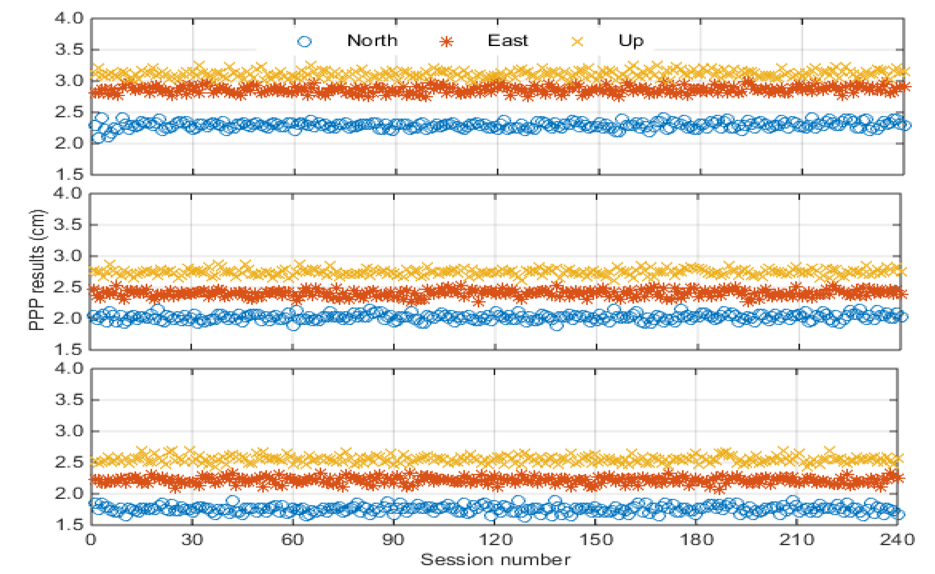
Figure 4.
Ten days (11 to 20 August 2014) positioning errors of strategies #1 (top), #2 (middle), and #3 (bottom) for 1-h sessions.
Figure 4.
Ten days (11 to 20 August 2014) positioning errors of strategies #1 (top), #2 (middle), and #3 (bottom) for 1-h sessions.

Figure 5.
1-h PPP estimations of the first session estimated with the three strategies.

Figure 6.
PPP results (cm) for the three coordinate components of north, east, and up, and the ratio values of the selected DD ambiguity processing.
Figure 6.
PPP results (cm) for the three coordinate components of north, east, and up, and the ratio values of the selected DD ambiguity processing.

Figure 7.
Residuals of the ionosphere-free phase combination of the PPP computation for the satellites of G16, G23, G27, and G31 of the stations of CMMZ (top), LGXC (middle), and SHJD (bottom).
Figure 7.
Residuals of the ionosphere-free phase combination of the PPP computation for the satellites of G16, G23, G27, and G31 of the stations of CMMZ (top), LGXC (middle), and SHJD (bottom).

Figure 8.
Results for the baseline components estimated with the DD algorithm for north (top), east (middle) and up (bottom) directions.
Figure 8.
Results for the baseline components estimated with the DD algorithm for north (top), east (middle) and up (bottom) directions.

Figure 9.
12 1-h PPP estimations of the two receivers for north, east, and up directions.


Table 1.
Settings for the precise point positioning (PPP) processing.
| Model | Settings | |
|---|---|---|
| Measurements | Ionosphere-free code and phase combination | |
| Adjustment | Least square | |
| Weighting | Elevation-dependent function | |
| Corrections | DCB(P1-C1) | Products provided by CODE |
| Tides corrections | Solid tide and ocean tide correction | |
| Phase center variation(PCV) | Absolute IGS 08 correction mode | |
| Relativity | Corrected | |
| Parameters | Station coordinates | Estimated |
| Troposphere | Correction: Saastamoinen model Residual: Estimate as piece wise mode | |
| Receiver clock error | Solved for at each epoch as white noise | |
| Phase ambiguity | Float and fixing results |
Table 2.
PPP solution Root mean square (RMS) (cm) of the three strategies using data from the local reference stations.
Table 2.
PPP solution Root mean square (RMS) (cm) of the three strategies using data from the local reference stations.
| Strategy | 1 h | 2 h | 4 h | ||||||
|---|---|---|---|---|---|---|---|---|---|
| North | East | Up | North | East | Up | North | East | Up | |
| #1 | 2.30 | 2.87 | 3.12 | 1.92 | 2.01 | 2.27 | 0.80 | 1.01 | 1.23 |
| #2 | 2.03 | 2.41 | 2.75 | 1.43 | 1.55 | 2.09 | 0.62 | 0.86 | 0.91 |
| #3 | 1.76 | 2.22 | 2.56 | 1.41 | 1.52 | 1.83 | 0.53 | 0.58 | 0.77 |
| Improvement (%) | 12 | 16 | 12 | 26 | 23 | 8 | 23 | 15 | 26 |
| 23 | 23 | 18 | 27 | 24 | 19 | 34 | 43 | 37 | |
Table 3.
PPP solution RMS (cm) of the three strategies using data from the regional reference stations.
Table 3.
PPP solution RMS (cm) of the three strategies using data from the regional reference stations.
| Strategy | 1 h | 2 h | 4 h | ||||||
|---|---|---|---|---|---|---|---|---|---|
| North | East | Up | North | East | Up | North | East | Up | |
| #1 | 2.28 | 2.89 | 3.15 | 1.93 | 2.03 | 2.25 | 0.80 | 1.01 | 1.23 |
| #2 | 2.09 | 2.44 | 2.79 | 1.47 | 1.58 | 2.10 | 0.62 | 0.86 | 0.91 |
| #3 | 1.71 | 2.19 | 2.53 | 1.38 | 1.49 | 1.83 | 0.53 | 0.58 | 0.77 |
| Improvement (%) | 8 | 16 | 11 | 24 | 22 | 7 | 23 | 15 | 26 |
| 25 | 24 | 20 | 28 | 27 | 19 | 34 | 43 | 37 | |
Table 4.
Baseline solution RMS (cm) of the two strategies using the local reference stations.
| Strategy | 1 h | 2 h | 4 h | ||||||
|---|---|---|---|---|---|---|---|---|---|
| North | East | Up | North | East | Up | North | East | Up | |
| #1 | 0.93 | 0.95 | 0.99 | 0.85 | 0.92 | 0.97 | 0.77 | 0.65 | 0.25 |
| #2 | 0. 89 | 0.90 | 0.91 | 0.80 | 0.88 | 0.91 | 0.76 | 0.64 | 0.22 |
| #3 | 0.84 | 0.85 | 0.89 | 0.78 | 0.82 | 0.88 | 0.72 | 0.60 | 0.20 |
| Improvement (%) | 4 | 5 | 8 | 6 | 4 | 6 | 1 | 2 | 12 |
| 10 | 11 | 10 | 8 | 11 | 9 | 6 | 8 | 20 | |
Table 5.
Baseline solution RMS (cm) of the two strategies using the regional reference stations.
| Strategy | 1 h | 2 h | 4 h | ||||||
|---|---|---|---|---|---|---|---|---|---|
| North | East | Up | North | East | Up | North | East | Up | |
| #1 | 0.94 | 0.96 | 0.98 | 0.86 | 0.91 | 0.98 | 0.78 | 0.64 | 0.26 |
| #2 | 0.90 | 0.90 | 0.89 | 0.81 | 0.87 | 0.93 | 0.76 | 0.63 | 0.23 |
| #3 | 0.85 | 0.87 | 0.89 | 0.77 | 0.82 | 0.89 | 0.71 | 0.62 | 0.19 |
| Improvement (%) | 4 | 6 | 9 | 6 | 4 | 5 | 3 | 2 | 12 |
| 10 | 9 | 9 | 10 | 10 | 9 | 9 | 3 | 27 | |
© 2018 by the authors. Licensee MDPI, Basel, Switzerland. This article is an open access article distributed under the terms and conditions of the Creative Commons Attribution (CC BY) license (http://creativecommons.org/licenses/by/4.0/).
Share and Cite
MDPI and ACS Style
Li, H.; Xiao, J.; Zhang, S.; Zhou, J.; Wang, J. Introduction of the Double-Differenced Ambiguity Resolution into Precise Point Positioning. Remote Sens. 2018, 10, 1779. https://doi.org/10.3390/rs10111779
AMA Style
Li H, Xiao J, Zhang S, Zhou J, Wang J. Introduction of the Double-Differenced Ambiguity Resolution into Precise Point Positioning. Remote Sensing. 2018; 10(11):1779. https://doi.org/10.3390/rs10111779
Chicago/Turabian StyleLi, Haojun, Jingxin Xiao, Shoujian Zhang, Jin Zhou, and Jiexian Wang. 2018. "Introduction of the Double-Differenced Ambiguity Resolution into Precise Point Positioning" Remote Sensing 10, no. 11: 1779. https://doi.org/10.3390/rs10111779
Note that from the first issue of 2016, this journal uses article numbers instead of page numbers. See further details here.