SMAP and CalCOFI Observe Freshening during the 2014–2016 Northeast Pacific Warm Anomaly


1
Jet Propulsion Laboratory/California Institute of Technology, Pasadena, CA 91109, USA
2
Physical Oceanography Department, Center for Scientific Research and Higher Education at Ensenada, 22860 Ensenada, Mexico
*
Author to whom correspondence should be addressed.
Remote Sens. 2018, 10(11), 1716; https://doi.org/10.3390/rs10111716
Submission received: 5 October 2018
/
Revised: 23 October 2018
/
Accepted: 26 October 2018
/
Published: 31 October 2018
(This article belongs to the Special Issue Sea Surface Salinity Remote Sensing)
Abstract
:Data from NASA’s Soil Moisture Active Passive Mission (SMAP) and from the California Cooperative Oceanic Fisheries Investigations (CalCOFI) were used to examine the freshening that occurred during 2015–2016 in the Southern California Current System. Overall, the freshening was found to be related to the 2014–2016 Northeast Pacific Warm Anomaly. The primary goal was to determine the feasibility of using SMAP data to observe the surface salinity signal associated with the warming and its coastal impact. As a first step, direct comparisons were done with salinity from the CalCOFI data at one-meter depth. During 2015, SMAP was saltier than CalCOFI by 0.5 Practical Salinity Units (PSU), but biases were reduced to <0.1 PSU during 2016. South of 33°N, and nearer to the coast where upwelling dominates, SMAP was fresher in 2015 by almost 0.2 PSU. CalCOFI showed freshening of 0.1 PSU. North of 33°N, SMAP and CalCOFI saw significant freshening in 2016, SMAP by 0.4 PSU and CalCOFI by 0.2 PSU. Differences between SMAP and CalCOFI are consistent with the increased stratification in 2015 and changes in the mixed layer depth. SMAP observed freshening that reached the Baja California Coast.
1. Introduction
A well-documented marine heat wave occurred in the Northeast Pacific during the period 2014–2016 (the 2014–2016 warm anomaly). Based on an analysis using NASA’s Multiscale Ultra-high-Resolution Sea Surface Temperature (MUR SST), [1] reported that SST anomalies along the West Coast of the United States were warmer than usual during the period 2014–2016, relative to the 2002–2012 climatology. They found that during the upwelling season, the anomalies were abated along the coast. As evidence of the regional effect of upwelling on the warming event, hydrographic data were used by [2] in finding that a strong upwelling event during the spring transition of 2015 abated the warm anomaly in Monterey Bay, California. The authors of [3], in their study of the pelagic ecosystem response of the 2014–2016 warm anomaly off Oregon, found the same effect of the strong upwelling event. Based on underwater gliders’ observations and ancillary data products, [4] found that during 2014–2015, the warming of the Southern California Current System (Southern CCS) was a combination of high downward heat flux and weak winds, conditions that also lead to the stratification of the water column. At the same time as the 2014–2016 warm anomaly, a strong El Niño event occurred. The work in [5] analyzed the influence of the 2015–2016 El Niño years on the CCS. They found that the effects of the equatorial Kelvin wave activity and the upwelling-favorable winds on the CCS were weaker than expected, especially for a strong El Niño. At the present time, a study of the salinity variability from remote sensing during the 2014–2016 warm anomaly is lacking.
The salinity signal associated with the 2014–2016 warm anomaly has been documented for some locations in the California Current domain by several authors. The work in [3] showed evidence of negative salinity anomalies for both surface and subsurface waters off the slope/shelf of Oregon. The works in [4] and [2] also found negative salinity anomalies off California. Recent results [6] have shown that salinity derived from the Soil Moisture Active Passive (SMAP) Mission can be used to detect changes in coastal waters associated with river discharge. In a study in the Gulf of Mexico, large signals in freshening were detected. The flooding event of 2015 in Texas caused an increase in river discharge, which led to a freshwater plume in the Gulf of Mexico and significant freshening of greater than five Practical Salinity Units (PSU). Changes in salinity of this magnitude could potentially have impacts on the biology [7]. The work outlined here seeks to determine, using the SMAP data, the observed surface salinity signal during the 2014–2016 warm anomaly. At the same time, direct comparisons will be made with the California Cooperative Oceanic Fisheries Investigations (CalCOFI) data.
A key issue, because of the comparison of remote sensing-derived surface salinity with in situ data, is how near-surface stratification can affect differences between the measurements. The issues were addressed by [8] where they examined possible differences between the two measurements due to evaporation, rain and specific types of wind conditions. Under low wind speeds and high evaporation, differences between one meter and the surface can reach at least 0.2 PSU. Thus, the interpretation of differences between remote sensing-derived salinity and in situ data must be interpreted with respect to the known stratification. This is critical in interpreting the validation of the results.
CalCOFI is a successful and enduring monitoring program, which includes a collection of hydrographic and biological data off the West Coast of North America. Since 1997, CalCOFI scientists have reported annually the state of the California Current. Their reports of 2015, 2016 and 2017 [9,10,11] have shown that the CalCOFI dataset is a very useful tool to study the hydrography of the 2014–2016 warm anomaly. The CalCOFI data have also been used to validate satellite products [12]. In particular, the CalCOFI hydrographic dataset has been used to evaluate the importance of in situ salinity observations in heat storage estimation from satellite altimetry [13]. To evaluate the performance of SMAP Sea Surface Salinity (SSS) during an open-ocean freshening event, this study compares SSS from SMAP with salinity (retrieved at one meter) from the CalCOFI array during the period 2015–2016. The variability of the freshening is examined along with explanations for differences between SMAP SSS and CalCOFI.
2. Materials and Methods
2.1. Methods
The work was divided into several steps:
- (1)
- Examination of the space-time variability of SSS from SMAP using Hovmöller diagrams.
- (2)
- Validation of SMAP SSS by direct comparisons with CalCOFI-derived salinity at a one-meter depth.
- (3)
- Evaluation of the space-time variability of salinity and stratification parameters associated with the warming event using CalCOFI data.
- (4)
- Evaluation of SMAP SSS versus CalCOFI salinity differences based on air-sea interaction.
For Step 1, Hovmöller diagrams based on latitude versus time were created from the SMAP SSS. The resolution of the SMAP SSS (40 km) allowed for an examination of the time-space evolution of the signal along the two longitudes: 118°W (see Figure 1), close to the coast, and at 120°W, further from the coast. The rationale was to see if there were differences in the variability associated with the coastal upwelling signal compared to further offshore. Additionally, the goal was to use the SMAP data to examine the propagation of the freshening signal from north to south. The two longitudes were chosen to determine if there was any spatial variability in the propagation of the signal as one got close to shore.
For Step 2, comparisons were done directly between the SMAP SSS and the CalCOFI salinity at a 1-m depth from April 2015–November 2016. The data were co-located in space-time using a simple nearest neighbor approach. Because SMAP is in an 8-day repeat orbit, the co-location window used was ±3 days and 25 km. As with Step 1, comparisons were divided into coastal and open ocean components. A simple criterion was used to divide coastal and open water stations (see Figure 1). For the sake of comparisons with the SMAP data, all CalCOFI stations within 100 km of the coast were considered coastal stations. For Step 3, Hovmöller diagrams were also derived directly using the CalCOFI data.
For the third step, we examined the space-time evolution of the freshening associated with the 2014–2016 warm anomaly. CalCOFI data were used to determine the full space-time evolution of the salinity signal associated with the warming event.
We based our analysis on using the CalCOFI data during the period 2003–2016. The CalCOFI data will be discussed more in Section 2.2.2. We used both basic statistics and analysis of anomalies. Basic statistics were obtained using the four CalCOFI surveys of each year. Temperature and salinity anomalies at the surface (1-m) depth were examined at CalCOFI Lines 76.7 (north), 83.3 (middle) and 90 (south) (see Figure 1), following the methodology of [14] and [15], which consists of the calculation of the mean seasonal variation based on the annual and semiannual harmonics for all stations, where the harmonics were obtained by a least-squares regression of the data. For each station, every anomaly was obtained relative to the mean seasonal variation and the 2003–2012 average. For mapping, Kriging interpolation was applied to the set of anomalies of each line of the CalCOFI sampling grid. Finally, Hovmöller diagrams were elaborated for each line.
For each line, the mixed layer depth was calculated following the method of [16]. The mixed layer depth anomalies were obtained following the same methodology as the one used with temperature and salinity anomalies.
As a final step, an evaluation was done of the air-sea interaction effect on the salinity variations. The rationale was to determine if differences between SMAP SSS and CalCOFI could be explained by the air-sea interaction. Following [17], a simple model was applied to evaporation and precipitation satellite-derived data. Assuming a balance between the salinity changes at the sea surface and the precipitation minus evaporation rates, the salinity budget equation is in the form:
where is the depth of the layer, is the mean surface salinity and and are the precipitation and evaporation rates, respectively. In this work, h = 1 m.
2.2. Data
2.2.1. JPL SMAP Data
The SMAP SSS data used in the study were from the JPL Version 3 product (doi:10.5067/SMP30-3TMCS).
The data were based on the Level 3 8-day running means gridded at a 0.25-degree resolution. The SMAP product, at the time of the study, was available from April 2015 through the end of 2016. The dates used overlapped with the CalCOFI data from spring 2015–fall 2016. More information on the data and its use may be found in the user’s guide [18]. Because of the proximity of the study area to land, a brief review of the data and the correction for land contamination set are given below.
Level 3 products are generated from the Level 2 products using a Gaussian weighting. Weights are assigned based on the distance to the center of the given grid cell. The Level 3 product also contains the Hybrid Coordinate Ocean Model (HYCOM) as an ancillary field, which is shown in the study for comparison purposes. More information on the HYCOM model may be found at https://www.hycom.org. The HYCOM model does not assimilate CalCOFI data. Information on the assimilated parameters used may be found at: https://hycom.org/attachments/084_5_Lozano.pdf. Briefly, parameters assimilated include sea surface temperature from the Advanced Very High Resolution Radiometer (AVHRR), geostationary GOES satellites and sea surface height from the Jason satellite. Low frequency boundary conditions are relaxed to climatologies, including temperature and salinity. HYCOM is used for comparison purposes with the JPL SMAP product to determine the influence of land contamination on the SMAP SSS retrieval. This is critical in a study that attempts to use SMAP SSS data to examine coastal dynamics such as upwelling. The land contamination issue is explained as follows. Radiometers measure energy from the entire visible disk seen on the Earth’s surface. If part of that disk lies over land, then the signal will partially include the brightness temperature generated by the land emissivity. In this case, the goal becomes to remove the signal due to land, leaving only the part due to the ocean. Corrections for land contamination are extremely important and need to be considered carefully when applying SMAP SSS to coastal studies.
To remove possible land contamination, the JPL SMAP product calculates a land climatology for the brightness temperature Tb at both the horizontal and vertical polarizations on a monthly time scale [18]. The climatology is then used to estimate the land contamination within 500 km of the coast. This is critical for deriving accurate SSS in the upwelling region off Southern California, which lies within areas of land contamination close to the coast. With the land correction, biases of SSS are reduced to −0.2 PSU with SSS being too fresh [18]. Beyond 50 km, biases are reduced to near zero. Root mean squared (RMS) differences are reduced to 0.5 PSU. Thus, the application of the land correction is critical for resolving the coastal SSS signal, where upwelling is expected to bring saltier deep water to the surface. Negative biases (fresher) near the coast would indicate possible land contamination.
2.2.2. CalCOFI Data
CalCOFI has made observations of the hydrography and biology off the West Coast of North America since 1949. Quarterly cruises have been conducted off Southern California since 1984. The CalCOFI’s standard sampling grid is based on parallel lines oriented perpendicular to the coast; the separation of lines and stations are both 74 km [14]. Data collected at depths down to 515 m include a Seabird 911 CTD (Conductivity, Temperature, Depth) mounted on a 24-bottle rosette with continuous measurements of pressure, temperature and conductivity. CalCOFI CTD data are computed by Seasoft based on (equation of state for seawater, 1980) EOS-80. Salinity is (practical salinity scale 1978) PSS-78. Salinity values in the CalCOFI array are typically between 32 and 36 PSU, with of course the equivalency of PSS and PSU. More information on CalCOFI CTD general practices and algorithms may be found at http://calcofi.org/. The modern CalCOFI salinity measurements provide a unique coastal dataset that spans decades. Thus, the data will provide a validation of SSS during the overlap period of the SMAP mission. Presented here is the time evolution of the seawater properties using data obtained during the 2003–2017 period in the CalCOFI 104 stations plan (see Figure 1). Details of the sampling protocol of this stations plan can be found in [14].
2.2.3. Evaporation Data
Evaporation data were retrieved from the Woods Hole Oceanographic Institution Objectively Analyzed Air-Sea Flux dataset [19]. More information on the dataset may be retrieved from http://oaflux.whoi.edu. The evaporation data use an advanced optimal interpolation technique to combine satellite and model from the numerical weather prediction. This is necessary because satellite data alone are not sufficient to derive parameters needed for the air-sea flux determination.
2.2.4. Precipitation Data
Rain rate was extracted from the Special Sensor Microwave Imager (SSM/I) onboard the Defense Meteorological Satellite Program (DMSP) satellites since 1987. DMSP satellites are polar orbiting and listed by satellite number, F08–F18. Rainfall data were downloaded from Remote Sensing Systems (http://www.remss.com/missions/ssmi/). More information on the processing and latest processing algorithms may be found in [20].
3. Results
3.1. Evaluation of SMAP Data
The JPL SMAP data were directly compared/co-located with all the CalCOFI data to determine the overall quality and validate the data in the region. The data were also divided into sub-regions for statistical comparisons to evaluate possible differences based on the proximity to the coast. For the SMAP and CalCOFI co-locations, we used the criterion of 100 km from the coast to delineate open ocean and coastal comparisons (see Figure 1). Comparisons were also done with the HYCOM model as a third independent dataset. The HYCOM model-derived salinity is readily available as an ancillary field in the SMAP SSS. Comparisons are only shown for the JPL product.
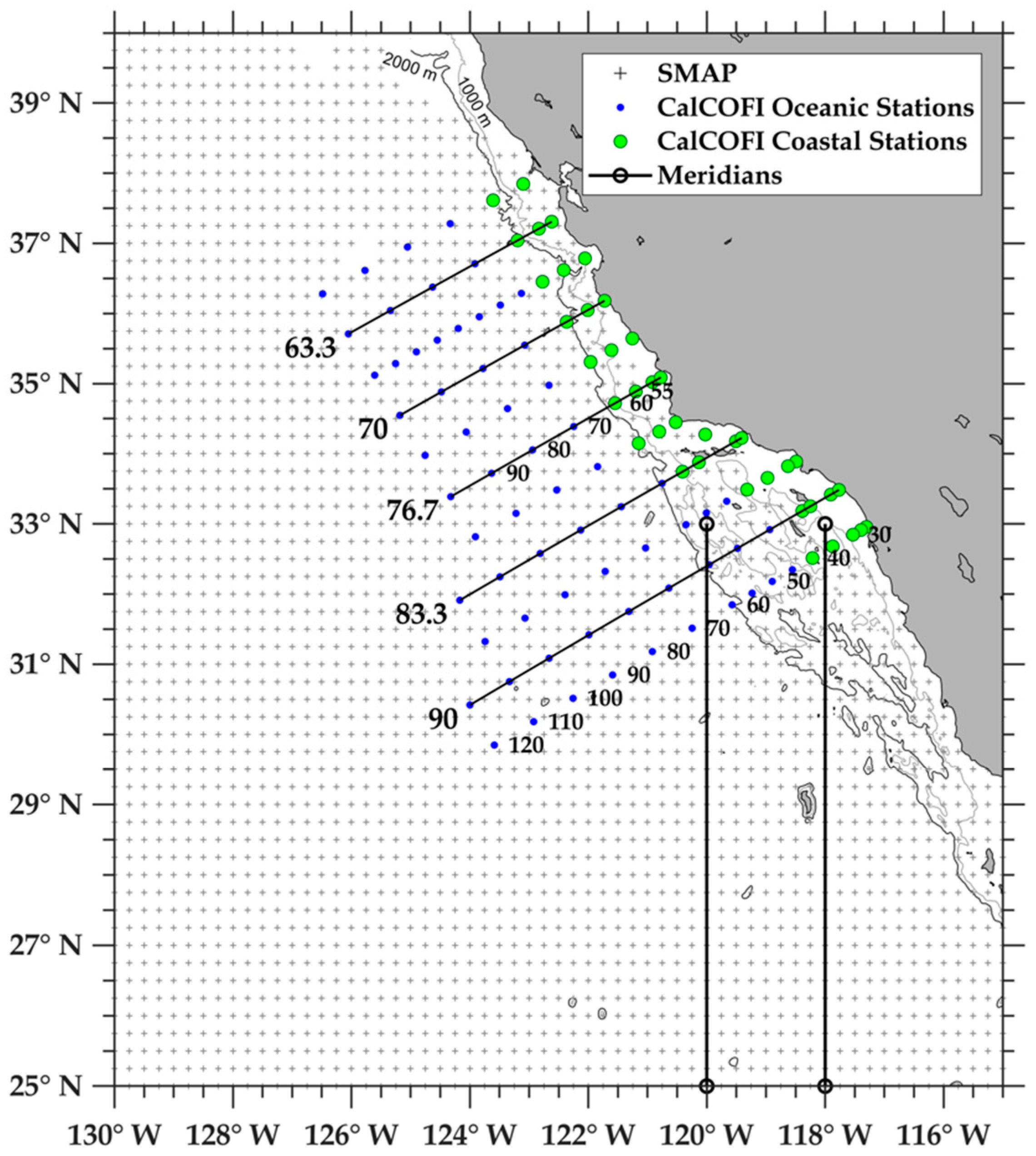
Figure 1 shows the location of the CalCOFI lines used in the study. Along the coast, the CalCOFI monitoring program spans the California Coastline. The stations’ plan also extends several hundred kilometers offshore. We analyzed all the lines shown in Figure 1. The lines 76.7, 83.3 and 90 had the highest occupations during the period 2003–2016.
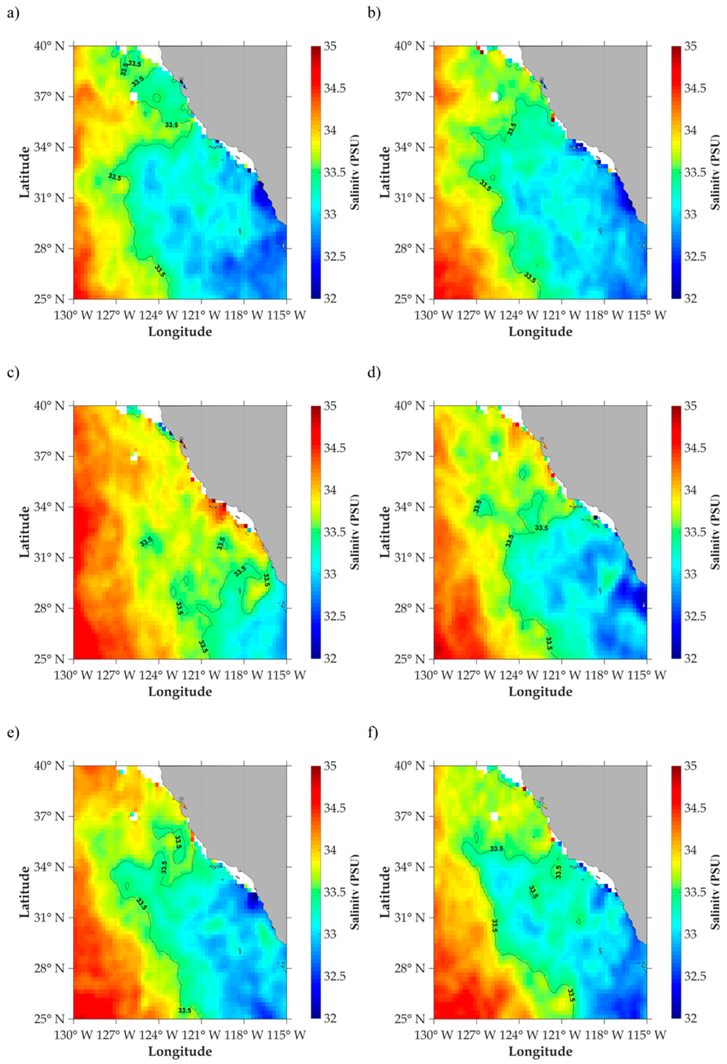
Figure 2a–f shows the monthly averaged values for SMAP for (a) April 2015, (b) April 2016, (c) July 2015, (d) July 2016, (e) November 2015 and (f) November 2016. The most prominent differences are clearly seen in July and November. July of 2015 clearly shows the saltier water along the coast associated with the seasonal upwelling. The work in [15] outlined three periods of upwelling off the Central to Northern California; April–June is associated with the intensification of upwelling due to alongshore Equatorward Winds. For July–September, one sees a relaxation of the upwelling associated with the weakening of the alongshore winds. November through March is considered the storm season and a transitional period. These patterns are consistent with the variability seen in Figure 2. Thus, the observed seasonal cycle in the SMAP SSS is consistent with the historical analysis. November of 2016 shows fresher waters along the coast, specifically between 30°N and 35°N. Overall, the SMAP SSS shows freshening from 2015–2016, with a clear impact along the coast and the upwelling signal seen in July. To our knowledge, this is the first time salinity data from SMAP have been used to observe the coastal upwelling signal off California that is associated with the 2014–2016 warm anomaly.
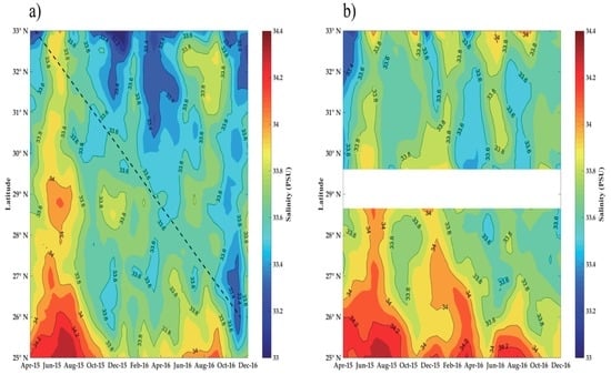
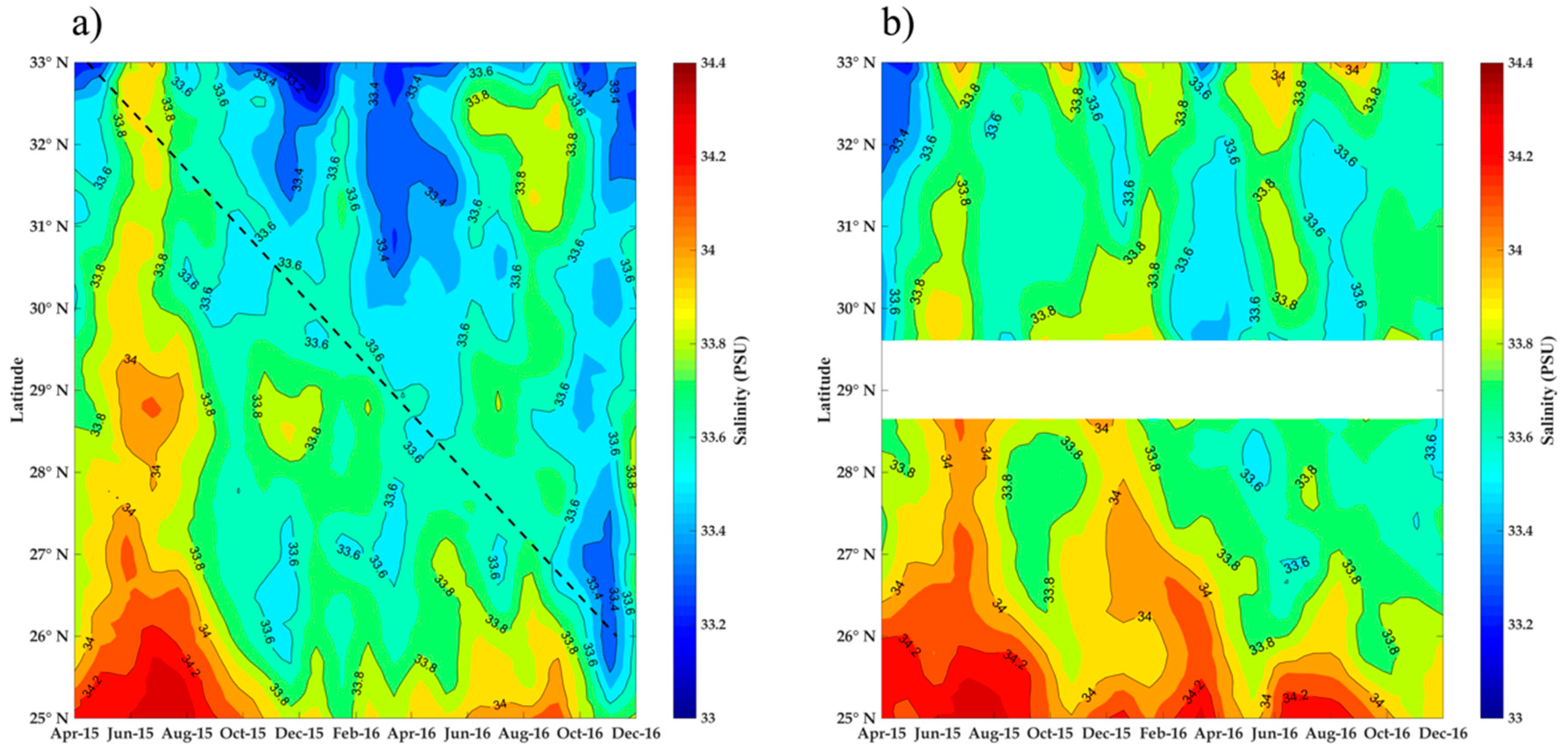
Figure 3a,b illustrates further the space-time variability of SSS from SMAP using Hovmöller diagrams at 120°W (a) and 118°W (b). Upwelling scales in this region can be variable, and the two longitudes were chosen based on work by [21]. The work in [21], for similar latitudes, chose 119°W to be representative of the coastal upwelling. Thus, the two longitudes were simply chosen to determine if there were changes in the propagation of the north-south freshening based on closeness to shore. At 120°W (further offshore), one clearly sees the propagation of freshwater from north to south, except during the summer and the seasonal upwelling season. From April 2015–December 2016, freshwater had propagated from 33°N–25°N. The dashed line in Figure 3a indicates a north-south propagation of approximately 2 cm/s. This is consistent with the observed effects of the warming off the Baja California Coast [22]. The work in [23] observed the propagation of the SST signal reaching the Baja California Coast. Freshening is also observed closer to the coast at 118°W, but the signal in 2015 is dominated by an annual/semiannual component, most likely due to the coastal upwelling signal. One still sees a semiannual component closer to the coast, but localized further south at approximately 25°N. The freshening has impacted the coastal waters and likely weakened the upwelling signal. The observed gap in data at approximately 29°N in Figure 3b is due to the island of Guadalupe. The results are consistent with [1] and [2] in showing that the warming along the coast abated during the spring upwelling season. Overall, the results are consistent in showing that although the impacts of the warming were felt along Southern California, and the maxima impact of SST and SSS were seen north of 35°N. Additionally, the saltier water seen near the coast for July 2015 is consistent with the 2015 El Niño [10]. To quantify and validate these results, direct comparisons were first made with the salinity at a one-meter depth from the CalCOFI monitoring program.
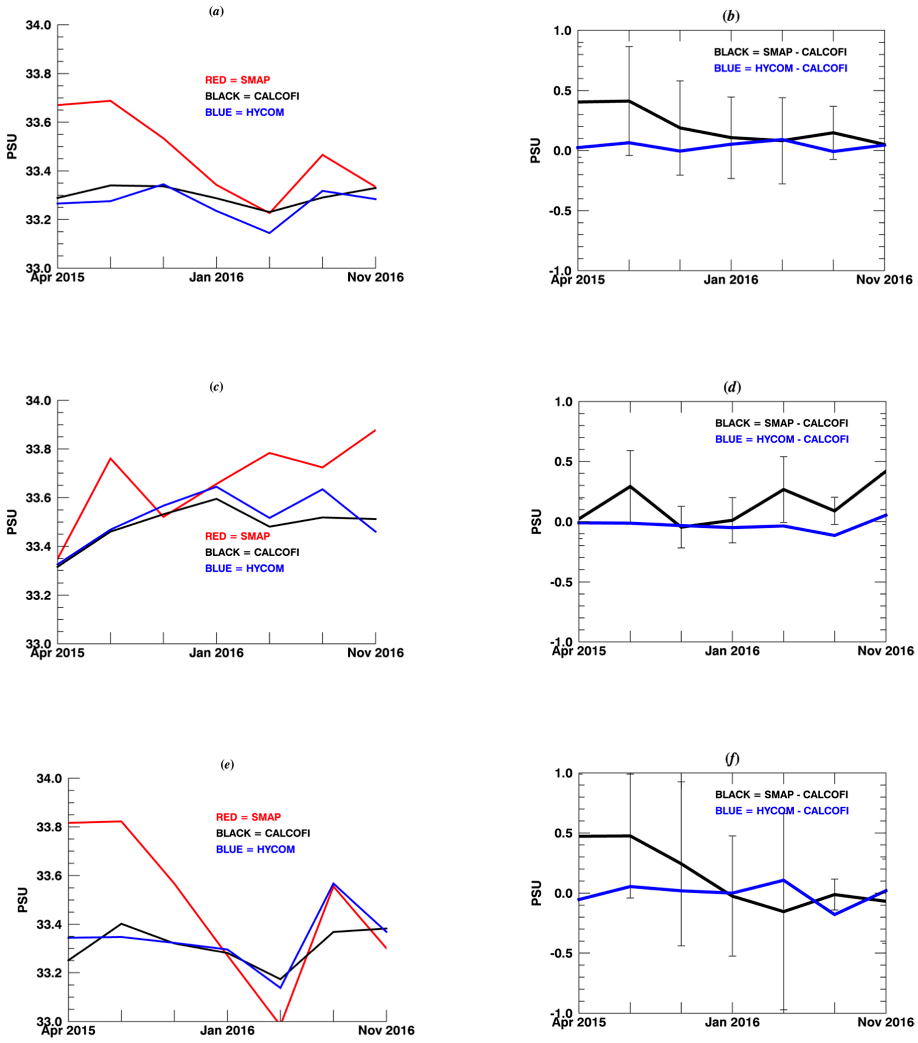
Figure 4 was generated using values of SMAP co-located with the CalCOFI lines from Figure 1. All the CalCOFI data indicated in Figure 1 were used. Results were separated into coastal and open ocean stations (see Figure 1). Figure 4a shows the mean SSS values over the entire CalCOFI region for April 2015, July 2015, November 2015, January 2016, April 2016 and November 2016. Over the entire region for 2015, values for SMAP SSS (red) were saltier than either HYCOM (blue) or CalCOFI (black). Values show SMAP SSS saltier by almost 0.4 PSU for 2015. In 2016, SMAP SSS and CalCOFI agreed to less than 0.1 PSU. Over the entire CalCOFI region, all three, SMAP, CalCOFI and HYCOM, showed a freshening from 2015–2016, but the freshening was magnified in SMAP. The freshening in SMAP was approximately 0.3 PSU, while in CalCOFI and HYCOM, the freshening was around 0.1 PSU. Figure 4b shows the bias between SMAP-CalCOFI (black) and HYCOM-CalCOFI (blue). Biases between HYCOM-CalCOFI were consistently smaller than 0.1 PSU over the entire region. Biases defined as SMAP-CalCOFI showed the saltier SMAP bias of 0.4 PSU for 2015 decreasing to less than 0.1 PSU in 2016. Thus, over the entire region, SMAP SSS was saltier than CalCOFI for 2015, almost reaching zero in 2016. Figure 4c is the same as Figure 4a, but for the area between 30°N and 33°N and using only the coastal stations (see Figure 1). The intent here was to focus on the upwelling region where also saltier SSS values were observed in July 2016 (see Figure 2). The latitudes 30°N and 33°N were chosen to capture the upwelling region (saltier) identified in Figure 2. Close to the coast (Figure 4c) in the Southern CCS region, all three: SMAP, CalCOFI, and HYCOM, showed fresher values in 2015, becoming slightly saltier in 2016. This is consistent with upwelling conditions returning to normal in mid–late 2016. SMAP shows an increase in saltiness by about 0.3 PSU, while CalCOFI and HYCOM show an increase of about 0.1 PSU. Figure 4e shows the SMAP, CalCOFI and HYCOM values for the region between 34°N and 38°N for the coastal stations only. All three datasets show an increase in freshening in 2016 with minimum values seen in April of 2016. However, the freshening in SMAP is even more pronounced, greater than 0.4 PSU. After April of 2016, all three datasets showed trends of increasing saltiness. Biases (Figure 4f) are reflective of the saltiness of SMAP in 2016. The change in the SSS trends between 30°N and 38°N would be consistent with the difference upwelling conditions associated with the California Coast. Error bars in Figure 4b,d,f show consistent RMS differences that are reduced to less than 0.3 PSU for 2016. Overall biases between the HYCOM SSS and CalCOFI SSS were <0.1 PSU. Based on Figure 4, the large salty bias in the SMAP SSS when compared with the CalCOFI in situ salinity will be addressed.
The saltier values of SMAP in 2015 may be understood in terms of the stratification of the water column. Previous studies comparing SMAP with ARGO data have shown that there are no significant changes in the biases between 2015 and 2016 [24]. There is also no indication that such biases exist in the CalCOFI data. Biases in satellite-derived SSS have other possible causes. Other possible explanations for the biases could be due to sea surface temperature [23]. However, the sea surface temperature biases dominate at cold temperatures [25]. This is due to the decreased sensitivity of salinity to changes in brightness temperatures. This bias would be minimized along the California Coast. Additionally, the bias would have a dominant seasonal cycle. As the largest biases occurred during the warmer waters of 2015, warm SST-induced biases effecting SSS are inconsistent with cold temperatures and a seasonal component. Thus, the sea surface temperature bias is an unlikely explanation for the differences seen between SMAP and CalCOFI. Another possible cause of biases is due to land contamination. However, maxima biases occurred at distances >100 km from the coast (open ocean), a distance that would not be associated with possible land contamination. Thus, another explanation must be found for the observed differences between 2015 and 2016. This will be discussed further in the next section with respect to the stratification of the water column and air-sea coupling. Overall results using the CalCOFI data showed increased stratification of the water column in 2015, with saltier values.
3.2. Salinity Variations Induced by Precipitation and Evaporation
Table 1 shows the year-to-year salinity changes associated with the rate of change of precipitation minus the evaporation factor. The change in salinity is based on using Equation 1. The maximum salinity change occurred in the fall and the minimum in summer. Because the evaporation rate was greater than precipitation rate, the salinity changes are mainly associated with the former. Table 1 reveals that the salinity changes in 2015 induced by the evaporation reached −0.6 PSU in April of 2015 and were greater than −2.2 PSU in November. The results are consistent with the saltier values derived from SMAP in 2015. The increased evaporation is also consistent with the increased stratification in 2015. This will be discussed more in later sections.
3.3. CalCOFI Observations
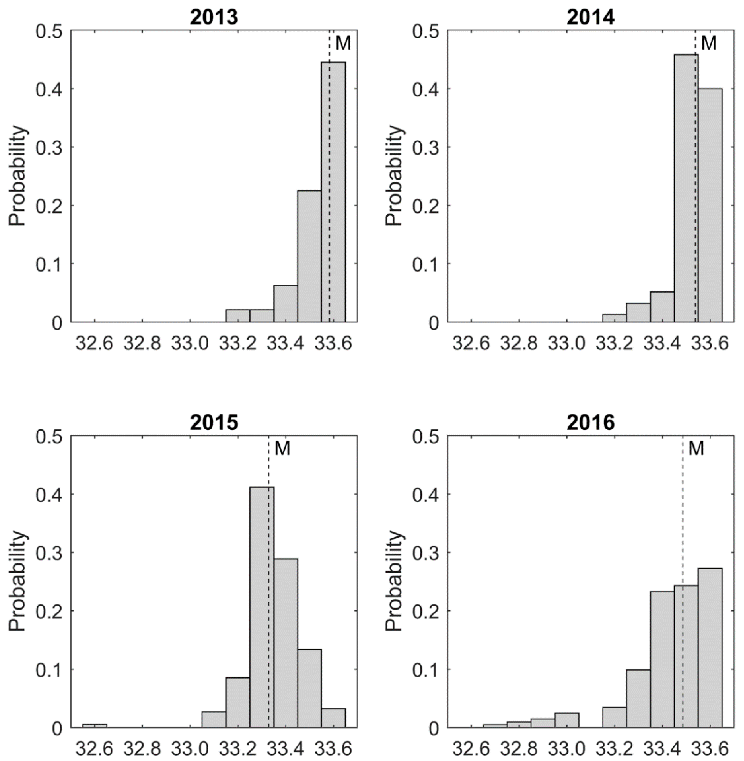
Figure 5 shows the histograms of the salinity distribution for the coastal zone at a 1-m depth for the four-year period 2013–2016. Station 60 of each line was used as the delimiter between the coastal and the oceanic zone. Because the arithmetic mean is sensitive to outliers, we used the median as the central tendency and higher central moments such as kurtosis and skewness to evaluate the dispersion. A positive kurtosis corresponds to a sharper peak, while the skewness is a measure of the asymmetry of the distribution. Whenever the distribution is extended more to the left of the mean value, it will always be a sign of a negative skew.
In 2013, the range of salinity was between 33.2 and 33.9 PSU with a skewness of −0.50 and a kurtosis of 4.9, while the median stood at 33.6 PSU (Table 2). In 2014, the range of the salinity was the same as in 2103, the skewness was −1.12, and the kurtosis was 5.1. In 2015, the range changed; it moved toward low values. The skewness value decreased, and the kurtosis increased, with the median decreasing. Finally, in 2016, the measures of central tendency and dispersion followed the same pattern as in 2015. The 2013–2014 period was saltier than the 2015–2016 period. It is also worth mentioning that the kurtosis was higher in the second period (2015–2016).
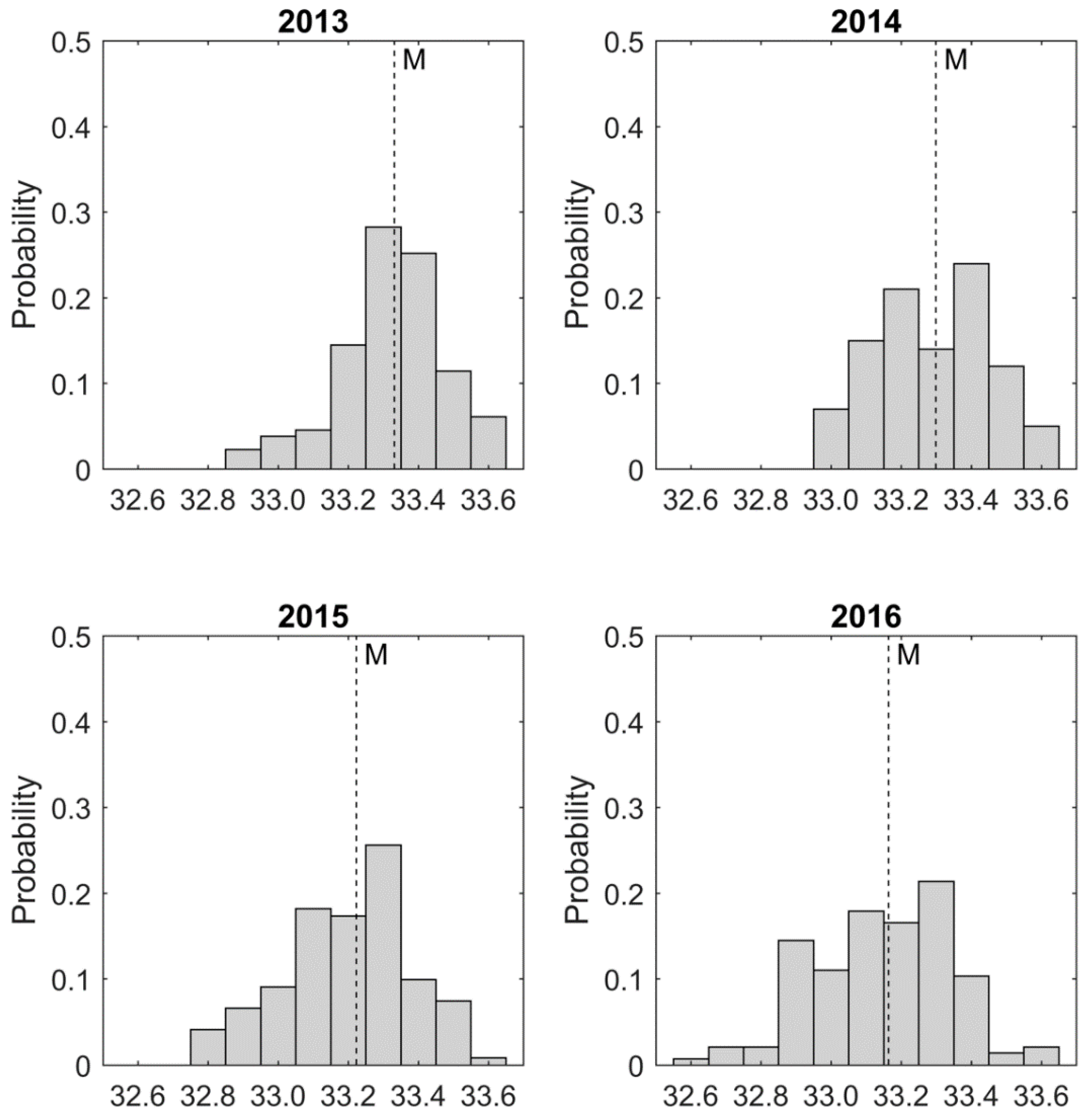
Figure 6 shows the histograms of the salinity distribution for the oceanic zone at a 1-m depth for the same four-year period. For the oceanic zone, these histograms show clearly the freshening from 2014 to the 2015–2016 period. In 2013, the range of salinity was between 32.8 and 33.7 PSU with a skewness of −0.30 and a kurtosis of 3.4, while the median stood at 33.3 PSU (Table 3). In 2014, the range of the salinity was the same as in 2013; the kurtosis was positive, and the median was larger than in 2013. In 2015, the range changed to 32.7–33.7 PSU; the skewness was −0.12, and the kurtosis increased to 2.3. In this case, the median decreased to 33.2 PSU. Finally, in 2016, the range of salinity was between 32.5 and 33.6 PSU; the skewness was −0.25; the kurtosis was 2.8; and the median decreased to 33.1.
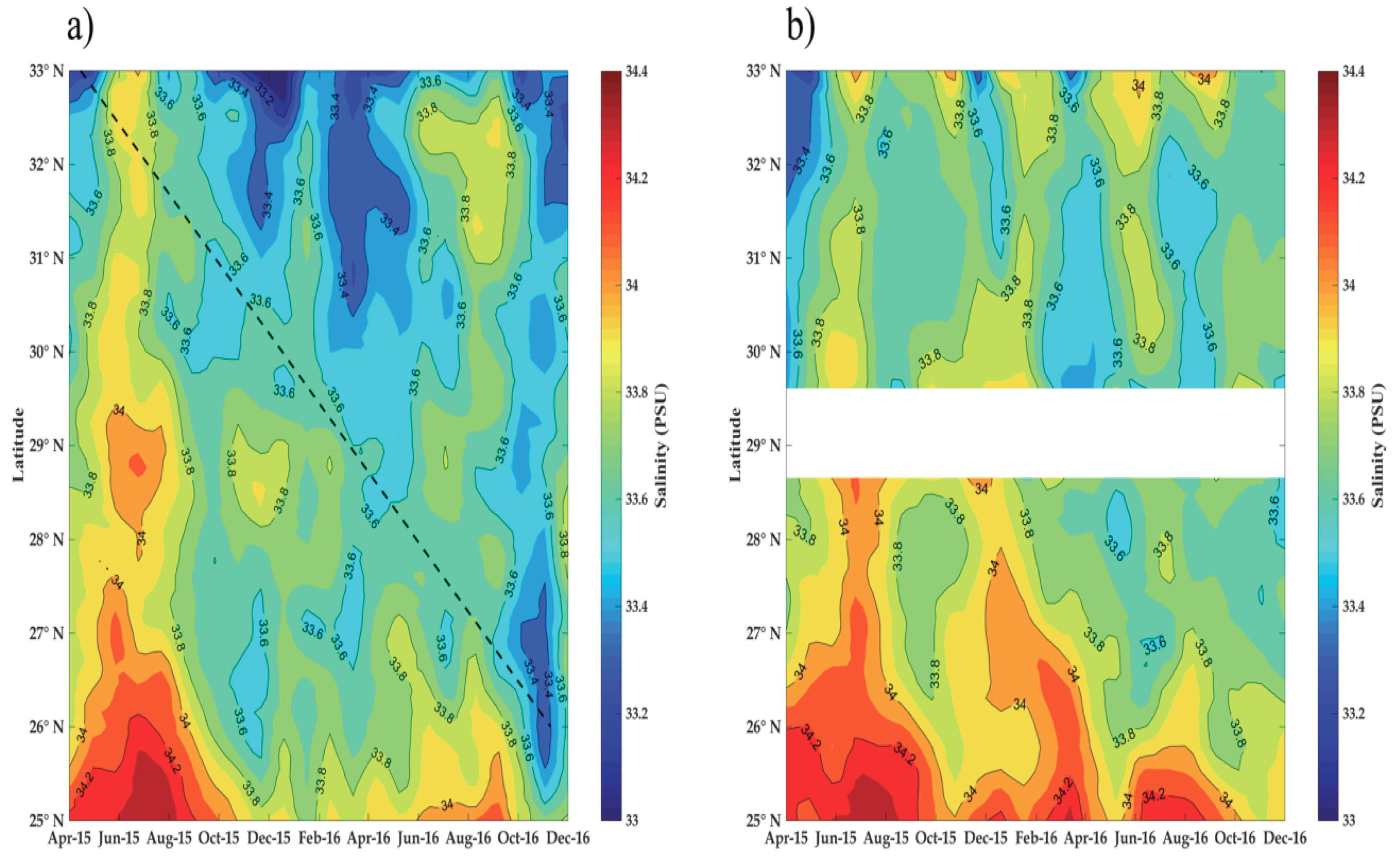
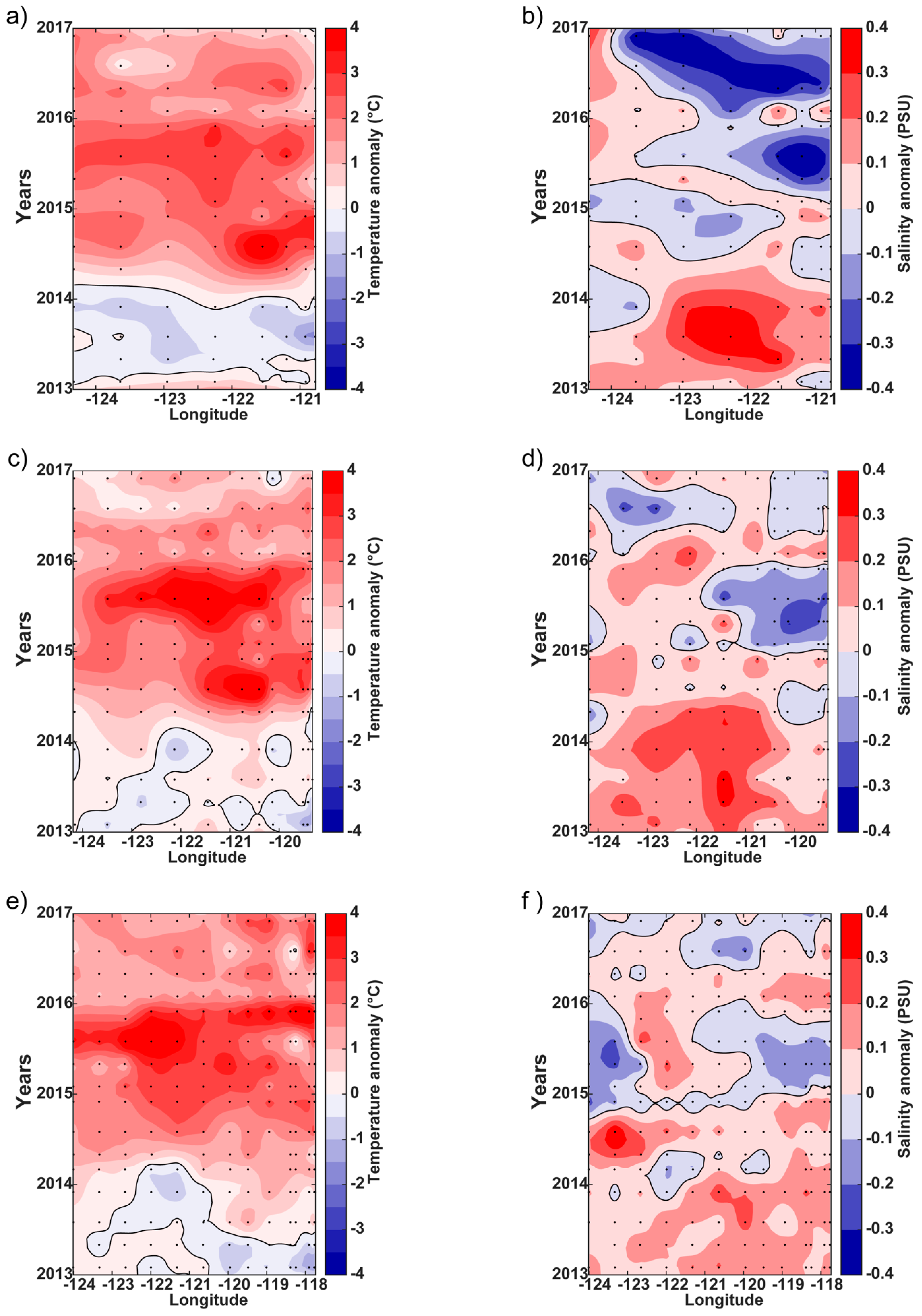
CalCOFI data at a 1-m depth registered the 2014–2016 warm anomaly (Figure 7a,c,e). In the CalCOFI region, the warming started in 2014 and was most pronounced in 2015 when the positive anomalies were around 4 °C.
The geographic distribution of SSS anomalies in the CalCOFI region was irregular during the period 2014–2016 (Figure 7b,d,f)), which is an indication that SSS was responsive to local dynamics and air-sea fluxes. Near the coast, negative SSS anomalies prevailed in 2015 at the three CalCOFI lines. In the northern part of the CalCOFI region (Line 76.7), negative SSS anomalies (less than −0.2 PSU) occurred in 2016 almost over the entire line, while for the rest of the CalCOFI lines’ negative SSS anomalies were of lesser magnitude. The minimum anomaly (−0.4 PSU) occurred in 2016 along Line 76.7. The freshening associated with the 2014–2016 warm anomaly was evident in the SSS anomalies.
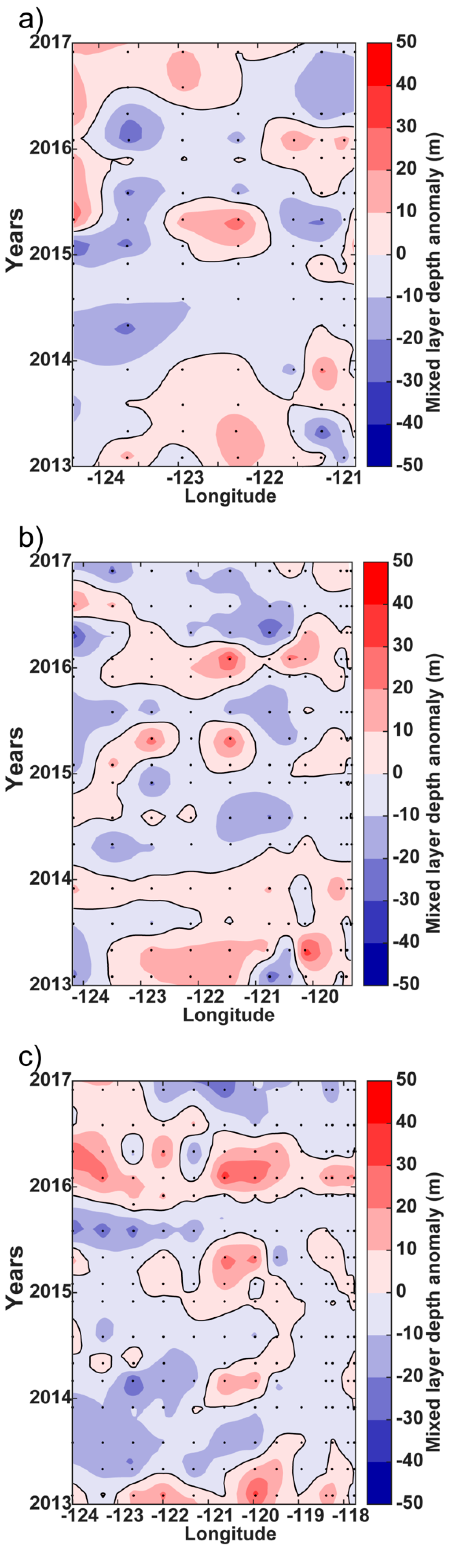
The Mixed Layer Depth (MLD) is an indication of the degree of stratification; the smaller the MLD, the greater the stratification. During the 2014–2016 warm anomaly, MLD was overall anomalously negative in the CalCOFI region (Figure 8a–c). At Line 76.7, the negative MLD anomalies prevailed during 2014–2015, when the highest number of negative anomalies occurred further from the coast. In exchange, the negative anomalies occurred near the coast in 2016. As for Line 83.3 the negative MLD anomalies also prevailed during 2014–2015, but not in the winter season. Meanwhile, at Line 90, the negative MLD anomalies were less abundant than the other lines. This would also be consistent with results from Figure 4, which showed that between 30°N and 33°N, the large biases between SMAP SSS and CalCOFI salinity were minimized, with both showing a trend to increasing saltiness in 2016.
4. Discussion
Results illustrate and compare both the surface salinity signal as measured by SMAP and the 1-m depth salinity signal as determined by CalCOFI during the 2014–2016 warm anomaly. Unique results are presented using SMAP SSS to observe the variability of salinity in a coastal region. Results are consistent with the CalCOFI 1-m depth salinity and the known stratification during that period of time.
Freshening was observed in the CalCOFI region throughout 2015 and 2016. The freshening was observed to be greater in the open ocean in both the CalCOFI and SMAP data. In the SMAP SSS, freshening offshore appears in 2015, spreading throughout the entire region in 2016. Offshore SMAP SSS shows freshening of 0.5 PSU starting in the north in 2015, but then extending south through 2016. The magnitude of the freshening, approximately 0.5 PSU, is most likely driven by the increased stratification in 2015. The stratification is consistent with MLD derivations for the same time period. Freshening is also observed in the CalCOFI lines, but at a decreased magnitude. Maximum freshening appears at Line 76.7 (north) in 2016 with anomalies, based on the CalCOFI climatology at one-meter depth, reaching 0.4 PSU. Further south, freshening is reduced with anomalies of 0.2 PSU appearing along the coast in 2015. The differences in SMAP SSS and CalCOFI salinity between 2015 and 2016 can be explained by the stratification of the water column. Stratification occurred in 2015 and 2016, but had a maximum in 2015. Biases between SMAP SSS and CalCOFI were larger than 0.4 PSU during 2015, but reduced to less than 0.1 PSU in 2016. The difference is consistent with the increased stratification in 2015. Results are consistent with [4], who showed that during the 2014–2015 period, local anomalous heat flux and wind strength led to the warming in the region. During the period of greater mixing and decreased stratification, differences between the SMAP SSS and CalCOFI were minimal. The stratification is consistent with increased evaporation rates in 2015 and changes in surface salinity.
Close to shore, both SMAP and CalCOFI show a trend towards saltier values between 2015 and 2016. This is consistent with the increasing strength of the upwelling signal in 2016. Results are consistent with [1] and [2].
Results are extremely important in showing that both satellite-derived SSS and in situ salinity are needed to monitor changes in the stratification of the water column associated with air-sea interactions. There are predominately two reasons for this. First, satellites measure a response at the surface of the ocean, while in situ measurements are at depth. Thus, differences between the two measurements would reflect the stratification of the water column, as they are related to the air-sea coupling. A second validation using in situ data is important in assessing the quality of the satellite data. Once validated, the satellites give enhanced spatial and temporal coverage not possible with in situ data. Off the California Coast, upwelling scales, along with fronts, can change on weekly to monthly time scales. The agreement between SMAP SSS and CalCOFI in the region is very encouraging for using SMAP SSS in coastal regions. Biases of less than 0.1 PSU would allow for monitoring of changes in salinity in critical ocean regions associated with coastal upwelling. SMAP is consistent in showing that near the coast, freshening was minimized. In 2015, the observed signal in freshening is consistent with a weakening of coastal upwelling [1,3].
Summarizing, direct comparisons between the SMAP SSS and salinity derived from the CalCOFI array showed that biases were observed with the SMAP SSS saltier than CalCOFI for 2015. During 2016, biases between SMAP SSS and CalCOFI were reduced to less than 0.1 PSU. One of the goals of the work was to determine the primary reason behind the observed differences between 2015 and 2016 and relate them to salinity differences between SMAP and CalCOFI caused by possible ocean conditions. Biases between the SMAP SSS and CalCOFI salinity could not be attributable to sea surface temperature and/or possible land contamination.
The 2015 differences between SMAP SSS and CalCOFI were found to be associated with the stratification of the water column. Based on the derivation, Figure 8 indicates a stronger stratification in 2015, consistent with an increase in salinity at the surface observed by the SMAP satellite. Differences in salinity between the two measurements are consistent with the results in [8].
5. Conclusions
Several key results were found from using the SMAP SSS. Overall, this should be considered an important step forward in applying satellite-derived salinity to coastal processes and their connection to basin-scale changes. We identified four major conclusions in the study. First, the SMAP SSS can be used to monitor the freshening in a coastal region associated with a major warming event. SMAP observed the freshening extending to the Baja California Coast. Second, using the SMAP SSS, freshening due to the Northeast Pacific heat wave was observed to propagate and reach the Baja California Coast. Third, the SMAP SSS identifies changes in salinity associated with a coastal upwelling system. Fourth, coastal station-based programs, such as CalCOFI, are critical for fully understanding and validating satellite-derived SSS. In periods of low stratification, biases between the SMAP-derived SSS and CalCOFI were less than 0.1 PSU, increasing to greater than 0.4 during periods of high stratification.
Parameters that identify the air-sea coupling are critical for a comprehensive understanding of the differences between satellite-derived and in situ surface salinities. This study shows that in situ data are not only needed for validation purposes, but also to understand fully the issues of stratification and mixing that may lead to differences between satellite-derived SSS and buoy salinity. Using both SMAP and CalCOFI leads to further evidence of the increased stratification during the 2014–2016 Northeast Pacific Warm Anomaly.
Future research should focus on validation efforts of SMAP in other coastal regions where upwelling is pronounced. This includes the Peru/Chile Coast, the Canarias, Benguela and Western Australia.
Supplementary Materials
Supplementary File 1Author Contributions
J.V.-C. carried out the work at the Jet Propulsion Laboratory as part of the Salinity Calibration/Validation effort. J.G.-V. carried out the work while on sabbatical at the Jet Propulsion Laboratory/California Institute of Technology from the Centro de Investigación Científica y de Educación Superior de Ensenada, Baja California. CONACyT supported the preparation of this paper through Contract No. 257125 to J.G.-V.
Funding
The lead author was funded through a contract with the National Aeronautics and Space Administration at the Jet Propulsion Laboratory/California Institute of Technology.
Acknowledgments
The research was carried out at the Jet Propulsion Laboratory, California Institute of Technology, under a contract with the National Aeronautics and Space Administration. The SMAP data are accessible through the Physical Oceanography Distributed Active Archive Center (https://podaac.jpl.nasa.gov/dataset/SMAP_JPL_L3_SSS_CAP_8DAY-RUNNINGMEAN_V3). CalCOFI data are available through http://calcofi.org/data.html. Luis E. Miranda, at the Centro de Investigación Científica y de Educación Superior de Ensenada (CICESE), gave computing and technical support to the project.
Conflicts of Interest
The authors declare no conflict of interest.
References
- Gentemann, C.L.; Fewings, M.L.; Garcia-Reyes, M. Satellite sea surface temperature along the West Coast of the United States during the 2014–2016 northeast Pacific marine heat wave. Geophys. Res. Lett. 2016, 44, 312–319. [Google Scholar] [CrossRef]
- Ryan, J.P.; Kudela, R.M.; Birch, J.M.; Blum, M.; Bowers, H.A.; Chavez, F.P.; Doucette, G.J.; Hayashi, K.; Marin, R., III; Mikulski, C.M.; Pennington, J.T.; et al. Causality of an extreme harmful algal bloom in Monterey Ba, California, during the 2014-2016 northeast Pacific warm anomaly. Geophys. Res. Lett. 2017, 44, 5571–5579. [Google Scholar] [CrossRef]
- Peterson, W.T.; Fisher, J.L.; Strub, P.T.; Du, X.; Risien, C.; Peterson, J.; Shaw, C.T. The pelagic ecosystem in the Northern California Current off Oregon during the 2014-2016 warm anomalies within the context of the past 20 years. J. Geophys. Res. Oceans 2017, 122. [Google Scholar] [CrossRef]
- Zaba, K.D.; Rudnick, D.L. The 2014–2015 warming anomaly in the Southern California Current System observed by underwater gliders. Geophys. Res. Lett. 2016, 43, 1241–1248. [Google Scholar] [CrossRef]
- Jacox, M.G.; Hazen, E.L.; Zaba, K.D.; Rudnick, D.L.; Edwards, C.A.; Moore, A.M.; Bograd, S.J. Impacts of the 2015–2016 El Niño on the California Current System. Early assessment and comparison to past events. Geophys. Res. Lett. 2006, 43, 7072–7080. [Google Scholar] [CrossRef]
- Fournier, S.; Reager, J.T.; Lee, T.; Vazquez-Cuervo, J.; David, C.H.; Gierach, M.M. SMAP observes flooding from land to sea: The Texas event of 2015. Geophys. Res. Lett. 2016, 43. [Google Scholar] [CrossRef]
- Pares-Escobar, F.; Lavaniegos, B.E.; Ambriz-Arreola, I. Interannual variability in oceanic euphausiid communities off the Baja California western coast during 1998–2008. Progr. Oceanogr. 2018, 160, 53–67. [Google Scholar] [CrossRef]
- Boutin, J.; Chao, Y.; Asher, W.E.; Delcroix, T.; Drucker, R.; Drushka, K.; Kolodziejczyk, N.; Lee, T.; Reul, N.; Reverdin, G.; et al. Satellite and in situ salinity: Understanding near-surface stratification and sub-footprint variability. Bull. Am. Meteorol. Soc. 2016. [Google Scholar] [CrossRef]
- Leising, A.W.; Schroeder, I.D.; Bograd, S.J.; Abell, J.; Durazo, R.; Gaxiola-Castro, G.; Bjorkstedt, E.P.; Field, J.; Sakuma, K.; Robertson, R.R.; et al. State of the California Current 2014–15: Impacts of the warm-water “blob”. Calif. Coop. Fish. Investig. Rep. 2015, 56, 31–68. [Google Scholar]
- McClatchie, S.; Goericke, R.; Leising, A.; Auth, T.D.; Bjorkstedt, E.; Robertson, R.R.; Brodeur, R.D.; Du, X.; Daly, E.A.; Morgan, C.A.; et al. State of the California Current 2015–2016: Comparisons with the 1997–98 El Niño. Calif. Coop. Fish. Investig. Rep. 2016, 57, 5–61. [Google Scholar]
- Wells, B.K.; Schroeder, I.D.; Bograd, S.J.; Hazen, E.L.; Jacox, M.G.; Leising, A.; Mantua, N.; Santora, J.A.; Fisher, J.; Peterson, W.T.; et al. State of the California Current 2016–17: Still anything but “normal” in the north. Calif. Coop. Fish. Investig. Rep. 2017, 58, 1–55. [Google Scholar]
- McClain, C.R. A decade of satellite ocean color observations. Annu. Rev. Mar. Sci. 2008, 1, 19–42. [Google Scholar] [CrossRef] [PubMed]
- Sato, O.T.; Polito, P.S.; Liu, W.T. Importance of salinity measurement in the heat storage estimation from TOPEX/POSEIDON. Geophys. Res. Lett. 2000, 27, 549–551. [Google Scholar] [CrossRef]
- Bograd, S.J.; Lynn, R.J. Long-term variability in the Southern California Current System. Deep-Sea Res. II 2003, 50, 2355–2370. [Google Scholar] [CrossRef]
- Garcia-Reyes, M.; Largier, J.L. Seasonality of coastal upwelling off central and northern California: New insights, including temporal and spatial variability. J. Geophys. Res. 2012, 117, C03028. [Google Scholar] [CrossRef]
- Torres, H.S.; Gomez-Valdes, J. Coastal Circulation driven by short-period upwelling-favorable winds in the northern Baja California region. Deep-Sea Res. I 2015, 98, 31–42. [Google Scholar] [CrossRef]
- Feng, M.; Hacker, P.; Lukas, R. Upper ocean heat and salt balances in response to a westerly wind burst in the western equatorial Pacific during TOGA COARE. J. Geophys. Res. 1998, 103, 10289–10311. [Google Scholar] [CrossRef] [Green Version]
- Fore, A.; Yueh, S.; Tang, W.; Hayashi, A. SMAP Salinity and Wind Speed Data User’s Guide; version 3; Jet Propulsion Laboratory/California Institute of Technology: Pasadena, CA, USA, 2016.
- Yu, L.; Jin, X.; Weller, R.A. Multidecadal Global Flux Datasets from the. Objectively Analyzed Air-sea Fluxes (OAFlux) Project: Latent and Sensible Heat Fluxes,. Ocean Evaporation, and Related Surface Meteorological Variables (OAFlux Project Technical Report OA-2008-01); Woods Hole Oceanographic Institution: Woods Hole, MA, USA, 2008; p. 64. [Google Scholar]
- Wentz, F.J. SSM/I Version-7 Calibration Report; RSS Technical Report 011012; Remote Sensing Systems: Santa Rosa, CA, USA, 2013; p. 46. [Google Scholar]
- Schwing, F.B.; O’Farrell, M.; Steger, J.M.; Baltz, K. Coastal Upwelling Indices West Coast of North America 1946-95; NOAA Technical Memorandum, NMFS, NOAA-TM-NMFS-SWFSC-231; United States Department of Commerce: Washington, DC, USA, 1996.
- Gómez-Ocampo, E.; Gaxiola-Castro, G.; Durazo, R.; Beier, E. Effects of the 2013–2016 warm anomalies on the California Current Phytoplankton. Deep-Sea Res. II 2017. [Google Scholar] [CrossRef]
- Di Lorenzo, E.; Mantua, N. Multi-year persistence of the 2014/15 North Pacific marine heat wave. Nat. Clim. Chang. 2016, 6. [Google Scholar] [CrossRef]
- Tang, W.; Fore, A.; Yueh, S.; Lee, T.; Hayashi, A.; Sanchez-Franks, A.; Martinez, J.; King, B.; Baranowski, D. Validating SMAP SSS with in situ measurements. Remote Sens. Environ. 2017, 200, 326–340. [Google Scholar] [CrossRef]
- Meissner, T.; Wentz, F.J.; Scott, J.; Vazquez-Cuervo, J. Sensitivity of Ocean Surface Salinity Measurements from Spaceborne L-Band Radiometers to Ancillary Sea Surface Temperature. IEEE Trans. Geosci. Remote Sens. 2016, 54, 7105–7111. [Google Scholar] [CrossRef]
Figure 1.
Map of the study area. Soil Moisture Active Passive Mission (SMAP) data domain (+) and location of the California Cooperative Oceanic Fisheries Investigations (CalCOFI) lines and stations. Coastal stations (<100 km) are denoted by green circles, and oceanic stations (>100 km) are denoted by blue circles. The isobaths for 1000 and 2000 m are contoured. Longitude lines 118°W and 120°W are highlighted.

Figure 2.
SMAP monthly. (a) Map of Sea Surface Salinity (SSS) averaged from SMAP for April 2015; (b) map of SSS averaged from SMAP for April 2016; (c) map of SSS averaged from SMAP for July 2015; (d) map of SSS averaged from SMAP for July 2016; (e) map of SSS averaged from SMAP for November 2015; (f) map of SSS averaged from SMAP for November 2016.

Figure 3.
(a,b) Hovmöller diagrams using SMAP-derived SSS of the latitudinal variation at two ((a) 120°W and (b) 118°W) longitudes. The dashed line shows the approximate propagation of the freshening from north to south.
Figure 3.
(a,b) Hovmöller diagrams using SMAP-derived SSS of the latitudinal variation at two ((a) 120°W and (b) 118°W) longitudes. The dashed line shows the approximate propagation of the freshening from north to south.

Figure 4.
(a) shows SSS averaged for the entire CalCOFI area defined in Figure 1 for coastal and open ocean stations. Salinity for all CalCOFI stations as measured by SMAP = red, CalCOFI = black and Hybrid Coordinate Ocean Model (HYCOM) = blue. (b) shows bias and RMS over the CalCOFI area for SMAP-CalCOFI (black) and HYCOM-CalCOFI (blue). (c) The same as (a), except for coastal stations between 30 and 33°N. (d) The same as (b), except for coastal stations between 30°N and 33°N. (e) The same as (a), except for coastal stations between 34°N and 38°N. (f) The same as (b), except for coastal stations between 34°N and 38°N.

Figure 5.
Histograms of salinity at a 1-m depth for the coastal zone of the CalCOFI sampling region: 2013, 2014, 2015 and 2016. The dashed line indicates the median of the distribution.
Figure 5.
Histograms of salinity at a 1-m depth for the coastal zone of the CalCOFI sampling region: 2013, 2014, 2015 and 2016. The dashed line indicates the median of the distribution.

Figure 6.
Histograms of salinity at a 1-m depth for the oceanic zone of the CalCOFI sampling region: 2013, 2014, 2015 and 2016. The dashed line indicates the median of the distribution.
Figure 6.
Histograms of salinity at a 1-m depth for the oceanic zone of the CalCOFI sampling region: 2013, 2014, 2015 and 2016. The dashed line indicates the median of the distribution.

Figure 7.
(a–f) Hovmöller diagrams of temperature anomalies (°C) at a 1-m depth for Lines 76.7 (a), 83.3 (c) and 90 (d) and salinity anomalies (PSU) at a 1-m depth for Lines 76.7 (b), 83.3 (e) and 90 (f). The anomalies are relative to the 2003–2012 climatology.
Figure 7.
(a–f) Hovmöller diagrams of temperature anomalies (°C) at a 1-m depth for Lines 76.7 (a), 83.3 (c) and 90 (d) and salinity anomalies (PSU) at a 1-m depth for Lines 76.7 (b), 83.3 (e) and 90 (f). The anomalies are relative to the 2003–2012 climatology.

Figure 8.
(a–c) Hovmöller diagrams of mixed layer depth anomalies (m) for Lines 76.7 (a), 83.3 (b) and 90 (c). The anomalies are relative to the 2003–2012 climatology.
Figure 8.
(a–c) Hovmöller diagrams of mixed layer depth anomalies (m) for Lines 76.7 (a), 83.3 (b) and 90 (c). The anomalies are relative to the 2003–2012 climatology.


Table 1.
Year-to-year salinity changes. PSU, Practical Salinity Units.
| Month | 2015–2016 (Units Are PSU) |
|---|---|
| January | −1.3 |
| April | −0.6 |
| July | 0.1 |
| November | −2.2 |
Table 2.
Year-to-year measures of central tendency and dispersion of the salinity distribution at a 1-m depth from the CalCOFI data for the coastal zone. Units are PSU.
Table 2.
Year-to-year measures of central tendency and dispersion of the salinity distribution at a 1-m depth from the CalCOFI data for the coastal zone. Units are PSU.
| Year | Range | Median | Skewness | Kurtosis |
|---|---|---|---|---|
| 2013 | 33.2–33.9 | 33.6 | −0.5 | 4.9 |
| 2014 | 33.2–33.6 | 33.5 | −1.1 | 5.1 |
| 2015 | 32.6–33.6 | 33.3 | −1.3 | 10.7 |
| 2016 | 32.3–33.7 | 33.5 | −2.3 | 10.0 |
Table 3.
Same as Table 2, except for the oceanic zone.
Table 3.
Same as Table 2, except for the oceanic zone.
| Year | Range | Median | Skewness | Kurtosis |
|---|---|---|---|---|
| 2013 | 32.8–33.7 | 33.33 | −0.30 | 3.48 |
| 2014 | 32.9–33.7 | 33.73 | −0.18 | 2.41 |
| 2015 | 32.7–33.7 | 33.22 | −0.12 | 2.67 |
| 2016 | 32.5–33.6 | 33.16 | −0.25 | 2.78 |
© 2018 by the authors. Licensee MDPI, Basel, Switzerland. This article is an open access article distributed under the terms and conditions of the Creative Commons Attribution (CC BY) license (http://creativecommons.org/licenses/by/4.0/).
Share and Cite
MDPI and ACS Style
Vazquez-Cuervo, J.; Gomez-Valdes, J. SMAP and CalCOFI Observe Freshening during the 2014–2016 Northeast Pacific Warm Anomaly. Remote Sens. 2018, 10, 1716. https://doi.org/10.3390/rs10111716
AMA Style
Vazquez-Cuervo J, Gomez-Valdes J. SMAP and CalCOFI Observe Freshening during the 2014–2016 Northeast Pacific Warm Anomaly. Remote Sensing. 2018; 10(11):1716. https://doi.org/10.3390/rs10111716
Chicago/Turabian StyleVazquez-Cuervo, Jorge, and Jose Gomez-Valdes. 2018. "SMAP and CalCOFI Observe Freshening during the 2014–2016 Northeast Pacific Warm Anomaly" Remote Sensing 10, no. 11: 1716. https://doi.org/10.3390/rs10111716
Note that from the first issue of 2016, this journal uses article numbers instead of page numbers. See further details here.