Intercomparison of In-Situ and Remote Sensing Salinity Products in the Gulf of Mexico, a River-Influenced System

Abstract

The recent emergence of satellite-based sea surface salinity (SSS) measurements provides new opportunities for oceanographic research on freshwater influence in coastal environments. Several products currently exist from multiple observing platforms and processing centers, making product selection for different uses challenging. Here we evaluate four popular SSS datasets in the Gulf of Mexico (GoM) to characterize the error in each product versus in-situ observations: Two products from NASA’s Soil Moisture Active Passive (SMAP) mission, processed by Remote Sensing Systems (REMSS) (40 km and 70 km); one SMAP 60 km product from the Jet Propulsion Laboratory (JPL); and one 60 km product from ESA’s Soil Moisture Ocean Salinity (SMOS) mission. Overall, the four products are remarkably consistent on seasonal time scales, reproducing dominant salinity features. Towards the coast, 3 of the 4 products (JPL SMAP, REMSS 40 km SMAP, and SMOS) show increasing salty biases (reaching 0.7–1 pss) and Root Mean Square Error (RMSD) (reaching 1.5–2.5 pss), and a decreasing signal to noise ratio from 3 to 1. REMSS 40 km generally shows a lower RMSD than other products (~0.5 vs. ~1.1 pss) in the nearshore region. However, at some buoy locations, SMOS shows the lowest RMSD values, but has a higher bias overall (>0.2 vs. <0.1 pss). The REMSS 70km product is not consistent in terms of data availability in the nearshore region and performs poorly within 100 km of the coast, relative to other products. Additional analysis of the temporal structure of the errors over a range of scales (8/9-day to seasonal) shows significantly decreasing RMSD with increasing timescales across products.

1. Introduction

Salinity dynamics are a critical component of marine systems that shape the physical environment and consequently influence ecosystem function by indirectly mediating biogeochemical processes. The structure and evolution of salinity patterns often have a significant role in setting stratification levels as well as influencing circulation patterns by affecting density gradients. This is particularly true in regions that are strongly influenced by river discharge. For example, freshwater associated with river plumes can have an influence on air–sea interaction through the formation of barrier layers, a layer near the surface with salinity stratification, but uniform temperature [1,2]. Barrier layers separate the density mixed layer above from the thermocline below, thus limiting the vertical mixing of heat between the mixed layer and the thermocline [3,4]. Rivers also supply a large amount of nutrients to the ocean, which can have an impact on biogeochemistry, ecology, and the carbon cycle [5,6]. As a result, improving the understanding of the impacts of river discharge on continental shelves and adjacent open ocean represent an active area of research in the oceanographic community.

Due to the importance of the upper ocean salinity structure, there have been notable efforts to improve the ability to map salinity patterns in the global ocean. In particular, satellite missions have provided unprecedented mapping capabilities of sea surface salinity (SSS) with spatiotemporal resolutions far beyond traditional in-situ measurement programs. Since 2010, SSS observations have been available from the European Space Agency’s (ESA’s) Soil Moisture and Ocean Salinity (SMOS) mission. During the period 2011–2015, the NASA’s Aquarius/SAC-D satellite mission was providing SSS measurements as well. Finally, since 2015, NASA’s Soil Moisture Active Passive (SMAP) mission also provides continuous SSS observations. From these satellite missions, several data products using different retrieval algorithms are currently available, with a range of spatial and temporal resolutions.

These products have been traditionally validated with in-situ data primarily in open ocean environments, for example, the Argo drifter program. Previous studies on the validation of SSS have focused on global validation using in-situ data [7,8,9]. Overall, Tang et al. [7] found that, on a monthly time scale, the Root Mean Square Error (RMSD) of SMAP SSS, when compared with Argo data, was approximately 0.2 pss. This is consistent with the global study of Lee, [8] which showed an accuracy of 0.2 pss for Aquarius SSS. Reference [9] also shows that the precision of the monthly SMOS SSS measurements is on the order of 0.2 pss globally. However, these statistics are based on global comparisons and there are only a few regional studies that evaluate the SSS observations with in-situ data in a coastal, river-influenced environment.

There have been some limited efforts to evaluate the capability of satellite SSS measurements in a few basin-scale studies. Reference [9] presents comparisons done in the Mediterranean with thermosalinograph (TSG) data and shows an average regional RMSD of 0.52 pss for SMOS SSS. Reference [10] evaluates SMAP SSS measurements in the Bay of Bengal and finds an average regional RMSD of 0.54 pss and a correlation coefficient of 0.81 when comparing SMAP to in-situ values. They also found the RMSD was dependent on distance from the coast, with RMSD increasing to 2 pss near the coast. Reference [11] also compares an early version of SMAP SSS measurements with in-situ data in the Gulf of Mexico (GoM) and finds an average regional RMSD of 1.36 pss over only a few months in 2015. Some other regional studies assessed SSS by comparison with other remote sensing datasets, such as altimetry, as well as in-situ data [12]. Reference [13] directly compares measurements of SMOS derived SSS with sea surface temperature from the National Oceanographic and Atmospheric Administration’s (NOAA’s) Advanced Very High-Resolution Radiometer in the Agulhas Retroflection Region. The comparison was done to examine the responses of salinity and sea surface temperature at the interannual time scales. Despite being less common, the regional evaluation of these products is critically needed, as modern research efforts push the limits of these products from global scale to regional and coastal science applications. However, to our knowledge, no regional study evaluates and intercompares different SSS products and their error characteristics for a river-influenced region.

With the current availability of remote sensing datasets that measure SSS, it is imperative to conduct regional validations that allow users to make decisions about the dataset which is best for their application. Here, we focus on assessing contemporary SSS products in a representative river-influenced system, namely the GoM. The GoM presents an opportunity to evaluate these products in a semi-enclosed basin with large temporal and spatial variability due to river discharge and advection from regional circulation. Typical of many riverine influence systems, the strong salinity gradients and highly variable conditions present in the GoM represent a markedly different environment than open ocean conditions that have slower temporal scales and larger spatial scales of variability. We highlight the performance of different satellite derived SSS data products from the SMAP and SMOS missions versus in-situ data over the period 2015–2017 in the GoM. In particular, this study assesses how well all the products reproduce the known seasonal and interannual cycles associated with river runoff and if there is a relationship between the quality of the SSS retrievals and distance from shore. This type of validation exercise, and its relationship to applications, are part of the crucial documentation needed by the user community for both research and applications to ensure the use of the most desirable dataset for their needs. Furthermore, understanding the performance of SSS products in the GoM is an important undertaking for regional interests, but more generally, it serves as an assessment of SSS product performance in a representative marine system strongly influenced by river discharge. The goal of this work is to provide statistics that can be used to conclude what products perform well for specific applications in the study region of the GoM.

Study Region

The GoM is a region that is influenced by large sources of both fresh and salty waters, resulting in large seasonal and interannual variability as well as strong horizontal and vertical salinity gradients within the system. The predominant source of freshwater in the northern GoM is the Mississippi River outflow, being the 6th large river system in the world [14]. In addition, there are other large freshwater sources across the northern GoM, including the Atchafalaya River, the Mobile Bay river system, the Apalachicola River, as well as numerous smaller rivers from Texas to Florida that can individually and collectively impact the freshwater inputs into the coastal ocean region [15,16,17]. For example, the effects of the Mississippi River discharge on the transport and fate of oil from the Deepwater Horizon Oil Spill have been a major topic of interest in the Gulf of Mexico [18]. On the opposite end of the salinity spectrum, the Loop Current brings high salinity waters (>35 pss) into the GoM at the southern boundary of the system via the channel between the Yucatan Peninsula and Cuba [19]. While the Loop Current flow path is generally in the eastern portion of the GoM, the system does shed westward propagating eddies, typically every 6–11 months [20,21]. As a result, the high salinity inputs from the Loop Current can impact large areas of the GoM. The interaction between coastal sources of freshwater and the Loop Current (and its associated eddies) leads to highly variable salinity fields that change over time at temporal scales of days to weeks to months [10,11,22,23]. Furthermore, this region of the ocean is typically underrepresented by the Argo drifter program, which has limited the SSS community’s ability to assess the quality of data products that are readily available. Overall, the different physical phenomena that affect salinity in the GoM make it an ideal basin for the validation of SSS products in a semi-enclosed basin.

2. Materials and Methods

2.1. Data

Our study focuses on SSS from a SMAP mission which is relatively new (beginning in 2015), and the longer term-SMOS satellite mission (2010–present) in our analysis to provide a comparison between different sensor products. In total, we examine 4 different satellite SSS products during the period 2015–2017 and details on each of these products are provided below. In addition, in-situ measurements of SSS from buoys and the World Ocean Database are also used as ground truth data in assessing the quality of the satellite SSS products. While there are inherent differences in the satellite SSS and the in-situ measurements, for example, depth of measurement (satellite SSS represent salinity in the top few cm of the ocean while in-situ salinity measurements are typically deeper than 1 m), spatial foot print, and so on, the combination of these two datasets provides a reasonable means of evaluating SSS product performance [12].

2.1.1. REMSS 40 km SMAP and REMSS 70 km SMAP

We used the Remote Sensing Systems SMAP Data Version 2.0 [24] from April 2015 to December 2017, distributed by Remote Sensing Systems (REMSS). Two versions of this data were used, a 40 km resolution product, and a 70 km resolution product, named REMSS SMAP 40 km and REMSS 70 km SMAP respectively in the following. Both products come as 8-day running means combining both ascending and descending orbits gridded on a 0.25 × 0.25 grid. More details on this SMAP product can be found in [24]. Briefly, the difference between the 40 km and 70 km is based on the smoothing radius. The smoothing is applied to the level 2 data and these values are then gridded onto the same 0.25° grid as the 40 km data. Global comparisons with HYCOM indicate that biases and RMSD are reduced in the 40 km dataset to 0 and 0.26 pss [24]. However, differences may exist regionally. Thus, both of these datasets were implemented in the validation study.

2.1.2. JPL SMAP

A third SMAP SSS product used in this study is the Level 3 Version 4.0, 8-day running mean SMAP SSS product distributed by the Jet Propulsion Laboratory, named JPL SMAP in the following. This product is a combination of ascending and descending orbits and also comes gridded on a 0.25 × 0.25 grid with an effective resolution of 60 km. More information on the data and their use may be found in the user’s guide [25], but the primary differences between this product and the REMSS 40 km relates to the application of different approaches to land contamination and smoothing of the overall product. The JPL SMAP product uses a land climatology to flag values for possible land contamination. As the GoM is an enclosed basin, this could lead to potential differences between the datasets. Quality flagging, gridding schemes based on the fore and aft views are also different between the two datasets. In the dual-view geometry, there is a forward scan from the satellite ground track position as well as an aft scan. Both scans are used to derive salinity measurements.

2.1.3. SMOS

We used the L3_DEBIAS_LOCEAN_v3 SMOS Sea Surface Salinity, produced by LOCEAN/IPSL (UMR CNRS/UPMC/IRD/MNHN) laboratory and ACRI-st company that participate in the Ocean Salinity Expertise Center (CECOS) of (French Ground Segment for the SMOS Level 3 and Level 4 data) Centre Aval de Traitement des Donnees SMOS (CATDS). This product is distributed by the Ocean Salinity Expertise Center (CECOS) of the CNES-IFREMER Centre Aval de Traitement des Donnees SMOS (CATDS), at IFREMER, Plouzane (France) [26]. The 0.25-degree maps are provided every 4 days from January 2010 to December 2017 and are derived from a combination of ascending and descending orbits. Debiased SSS are temporally averaged using a slipping Gaussian kernel with a full width at half maximum of 9 days. A median filtering over nearest neighbors is applied. Based on the smoothing and filtering, the effective resolution of the SMOS is 60 km, similar to the JPL SMAP product. This similarity in smoothing is important for interpreting the statistical comparisons with the buoys and the World Ocean Database (WOD).

2.1.4. In-Situ Data

The availability of coastal in-situ data is critical for these types of comparisons. In regional basins, the temporal and spatial coverage of the Argo drifter program is often not sufficient to resolve shelf and shelf-open ocean processes. As a result, this study focuses on two sets of in-situ data, measurements from continuous surface buoys, as well as observations of opportunity from the WOD, which address, to some extent, the limitation of typical SSS validation efforts. The buoy data are collected from 7 buoys in the eastern and western shelves of the GoM. Measurements were made every 0.5–1.0 h, from which daily averages were produced for comparisons with the satellite SSS data. The data are part of the NOAA National Data Buoy Center (NDBC) and may be retrieved from (https://www.ndbc.noaa.gov/) and the Texas Automated Buoy System (TABS) (http://tabs.gerg.tamu.edu/). The west Florida shelf buoys acquire data at 1 m deep and the Texas buoys at 1.8 m [27]. In the following we refer to these buoy data as buoy SSS.

Data from the WOD were retrieved directly from NOAA’s National Oceanographic Data Center (NODC) (now part of the National Centers for Environmental Information (NCEI) https://www.nodc.noaa.gov/OC5/WOD/pr_wod.html). Data from the WOD include conductivity/temperature/depth (CTDs), gliders, profilers, and drifting buoys and provide a unique opportunity for validation in a coastal/regional basin. Here, we use the salinity in-situ measurements from the 1–9 m depth range in order to have more in-situ near-surface observations. In the following, we refer to these WOD in-situ near-surface measurements as WOD SSS. The WOD2013 contains the full set of quality controls. Updates from April 2013 to the present implement the initial quality controls.

2.2. Methodology

To get a broad sense of the systematic performance between products, means and their associated standard deviations are derived from the REMSS 40 km SMAP, REMSS 70 km SMAP, JPL SMAP, and SMOS products. Record-length and seasonal means are calculated from the start of the SMAP mission in April 2015 through the end of 2017. Winter is defined as the monthly averages for January, February, and March; spring as the monthly averages for April, May, and June; summer as the monthly averages for July, August, and September; fall as the monthly averages for October, November, and December. Standard deviations are calculated based on the same periods of time.

To validate the accuracy of the satellite SSS products, comparisons were made directly with the seven buoys and data from the WOD. Figure 1 shows a map of the density of the WOD SSS from April 2015 through the end of 2017. Most available data are located in the northern part of the GoM and the density is higher along the shelf. Overlaid on the map are the locations of the 7 buoys, 4 on the Texas shelf and 3 along the coast of Florida.

We collocated the 7 buoys with satellite SSS using the nearest neighbor location. Comparisons between the SSS products and the buoys were made at three-time scales: Daily/8-day, 31-day, and 91-day time scales. SMAP SSS data have a temporal resolution (repeat orbit) of 8-day. SMOS has a temporal resolution of 9-day. It has an exact repeat of 149 days with a subcycle of 18 days and a revisit time of 3 to 5 days. Nine days was chosen because it is half of the SMOS subcycle and close to one week.

These were compared with the daily buoy SSS data, as the complete coverage of satellite SSS is completed in 8–9 days. For the 31- and 91-day time scales, SSS and buoys SSS data were smoothed using a running mean with a window of +/−15 and +/−45 days, respectively. Statistics were then calculated for the daily/8-day running means, as well as 31-day and 91-day smoothed results. The rationale for different averaging schemes was to examine whether smoothing over the monthly and seasonal time scales significantly change product quality.

Concerning the WOD SSS, the subsetting capability was used to extract all the data that overlapped from the start of the SMAP mission data availability (April 2015) through the end of 2017. All the data were extracted in the region from 18°N to 32°N and 100°W to 80°W. The co-location between satellite and WOD in-situ SSS was made using a nearest neighbor approach as well. Note that near-surface salinity stratification in the upper few meters can contribute to differences between satellite (for the top cm) and in-situ SSS at these depths [12].

Below are the definitions we used for the root mean square difference (RMSD) and signal to noise ratio. RMSD was based on the co-located satellite derived products and in-situ data. RMSD is then calculated as:

$$RMSD=\sqrt{\frac{\sum {\left(satellite SSS-in situ SSS\right)}^2}{n total}}$$

(1)

where n total is the total number of points for the summation. The signal to noise ratio (SN) can then be defined as:

$$SN=\frac{STDs}{RMSD}$$

(2)

where STDs is the standard deviation of the satellite product defined as:

$$STDs=\sqrt{\frac{\sum {\left(satellite-mean sat\right)}^2}{n total}}$$

(3)

where mean sat is the mean of the SSS derived from the satellite product over the n total points. It is important that we used the STD of the satellite product to define the signal. As defined by the variability measured by the satellite, the signal will not include missing subpixel scale variability. It will include, of course, noise in the data, due to instrument error, land contamination, and other factors in determining SSS from the satellite. Thus, the signal to noise estimate is a best estimate, based on using the satellite measurements and the WOD.

Figure 1 shows the density of the WOD salinity data. A considerable amount of the northern GoM is covered for the period of time between April 2015 and December 2017. Overlaid on the map are also 7 independent buoys that are used in comparisons with the 4 SSS products. Following the naming convention of the buoys, the 7 buoys are labeled C10, C12, C13, F, X, V, and K. Each buoy consists of a time series of surface salinity, which spanned the 2015–2017 time frame. However, the starting time, as well as data gaps, vary for each buoy. As a result, the 3 buoys (2 western and 1 eastern gulf locations) with the most complete time records are highlighted in the section below. However, the overall statistics for all the buoys are shown in

Table 1. Statistics of the comparisons between each satellite product (SMOS, JPL SMAP, REMSS SMAP, and REMSS SMAP 70 km) and buoy salinity data. The locations of the buoys are indicated in Figure 6.

Buoy	Satellite Dataset	Bias (pss)	RMSD (pss)	Correlation
Buoy C10	JPL 8-day	0.24	0.78	0.62
	JPL 31-day	0.24	0.66	0.67
	JPL 91-day	0.26	0.50	0.69
	REMSS 40 km 8-day	−0.23	0.61	0.13
	REMSS 40 km 31-day	−0.24	0.42	0.30
	REMSS 40 km 91-day	−0.10	0.35	0.50
	REMSS 70 km 8-day	N/A	N/A	N/A
	REMSS 70 km 31-day	N/A	N/A	N/A
	REMSS 70 km 91-day	N/A	N/A	N/A
	SMOS 9-day	N/A	N/A	N/A
	SMOS 31-day	N/A	N/A	N/A
	SMOS 91-day	N/A	N/A	N/A
Buoy C12	JPL 8-day	−0.21	0.44	0.89
	JPL 31-day	−0.21	0.26	0.94
	JPL 91-day	−0.20	0.19	0.95
	REMSS 40 km 8-day	−0.12	0.49	0.86
	REMSS 40 km 31-day	−0.12	0.33	0.92
	REMSS 40 km 91-day	−0.11	0.25	0.93
	REMSS 70 km 8-day	−0.10	0.62	0.69
	REMSS 70 km 31-day	−0.09	0.51	0.74
	REMSS 70 km 91-day	−0.08	0.37	0.80
	SMOS 9-day	−0.01	0.43	0.90
	SMOS 31-day	−0.02	0.19	0.98
	SMOS 91-day	−0.01	0.12	0.99
Buoy C13	JPL 8-day	−0.13	0.40	0.81
	JPL 31-day	−0.13	0.25	0.91
	JPL 91-day	−0.12	0.20	0.92
	REMSS 40 km 8-day	−0.09	0.47	0.72
	REMSS 40 km 31-day	−0.09	0.31	0.75
	REMSS 40 km 91-day	−0.07	0.23	0.88
	REMSS 70 km 8-day	−0.09	0.54	0.56
	REMSS 70 km 31-day	−0.09	0.40	0.68
	REMSS 70 km 91-day	−0.08	0.25	0.83
	SMOS 9-day	−0.03	0.33	0.85
	SMOS 31-day	−0.03	0.19	0.94
	SMOS 91-day	−0.02	0.14	0.95
Buoy F	JPL 8-day	0.43	1.25	0.91
	JPL 31-day	0.45	0.58	0.97
	JPL 91-day	0.51	0.43	0.98
	REMSS 40 km 8-day	0.04	0.90	0.85
	REMSS 40 km 31-day	0.02	0.65	0.87
	REMSS 40 km 91-day	0.13	0.89	0.75
	REMSS 70 km 8-day	N/A	N/A	N/A
	REMSS 70 km 31-day	N/A	N/A	N/A
	REMSS 70 km 91-day	N/A	N/A	N/A
	SMOS 9-day	0.57	1.12	0.87
	SMOS 31-day	0.60	0.61	0.96
	SMOS 91-day	0.66	0.39	0.96
Buoy K	JPL 8-day	0.25	1.13	0.80
	JPL 31-day	0.28	0.54	0.93
	JPL 91-day	0.29	0.45	0.90
	REMSS 40 km 8-day	0.23	1.10	0.83
	REMSS 40 km 31-day	0.21	0.52	0.94
	REMSS 40 km 91-day	0.14	0.60	0.89
	REMSS 70 km 8-day	−0.06	1.23	0.68
	REMSS 70 km 31-day	−0.25	0.25	0.94
	REMSS 70 km 91-day	−0.25	0.45	0.70
	SMOS 9-day	−0.16	1.04	0.83
	SMOS 31-day	−0.15	0.33	0.97
	SMOS 91-day	−0.13	0.26	0.97
0.Buoy V	JPL 8-day	−0.43	0.78	0.88
	JPL 31-day	−0.43	0.54	0.93
	JPL 91-day	−0.43	0.39	0.93
	REMSS 40 km 8-day	−0.22	0.87	0.87
	REMSS 40 km 31-day	−0.22	0.61	0.92
	REMSS 40 km 91-day	−0.23	0.45	0.93
	REMSS 70 km 8-day	−0.25	0.77	0.89
	REMSS 70 km 31-day	−0.25	0.53	0.94
	REMSS 70 km 91-day	−0.25	0.38	0.94
	SMOS 9-day	−0.66	0.59	0.93
	SMOS 31-day	−0.66	0.29	0.98
	SMOS 91-day	−0.66	0.20	0.98
Buoy X	JPL 8-day	−0.18	0.37	0.30
	JPL 31-day	−0.19	0.27	0.50
	JPL 91-day	−0.18	0.24	0.56
	REMSS 40 km 8-day	0.07	0.33	0.38
	REMSS 40 km 31-day	0.06	0.21	0.55
	REMSS 40 km 91-day	0.05	0.25	0.42
	REMSS 70 km 8-day	−0.17	0.39	−0.01
	REMSS 70 km 31-day	−0.19	0.25	−0.30
	REMSS 70 km 91-day	−0.16	0.22	−0.57
	SMOS 9-day	−0.50	0.24	0.69
	SMOS 31-day	−0.55	0.14	0.88
	SMOS 91-day	−0.64	0.18	0.77

. Results will be elaborated on in the Discussion section. The issue of the quality of retrievals based on proximity to land will also be addressed in the Discussion section. The issue of stratification and biases in the SMOS data has been addressed by Reference [12]. Results here build on those presented in Reference [28] in the Gulf of Mexico.

3. Results

3.1. Climatologies and Seasonal Variability

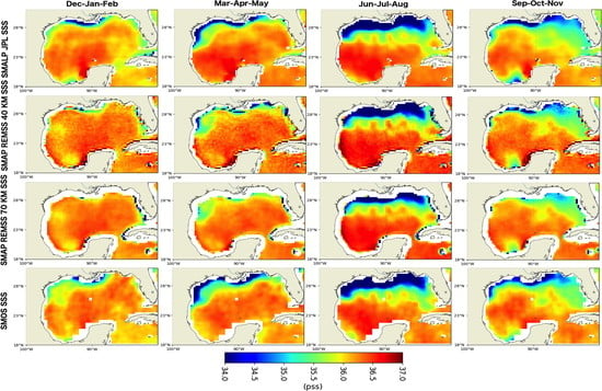
Figure 2 and Figure 3 show the seasonal means and standard deviations of the REMSS 40 km and 70 km SMAP, JPL SMAP, and SMOS products, respectively, for the four datasets in winter, spring, summer, and fall (see Materials and Methods section). All four datasets clearly show maximum freshening in the northern GoM in the summer time frame. The seasonal cycle is consistent with previous results reported by Fournier et al. [11]. Freshening starts in the spring, reaching its maximum in summer, with a large tongue of freshwater extending offshore in the eastern GoM associated with the Mississippi River plume. However, differences in the datasets do exist primarily in the coastal regions. Freshening is clearly visible, starting in the spring time frame for the JPL SMAP, REMSS SMAP 40 km and 70 km, and SMOS. However, freshening in spring is difficult to identify in the REMSS 70 km SMAP product. This can be explained by the smoothing that occurs in the REMSS 70 km SMAP product and the proximity to land. White in the images indicates missing data in the product due to land contamination. The area associated with land contamination in the REMSS 70 km SMAP product extends further from the coast, thus masking the majority of spring time freshening. The same issue is seen in the fall means, where the fresher conditions along the northern GoM coast are masked out. Overall, all four datasets show remarkably good comparisons.

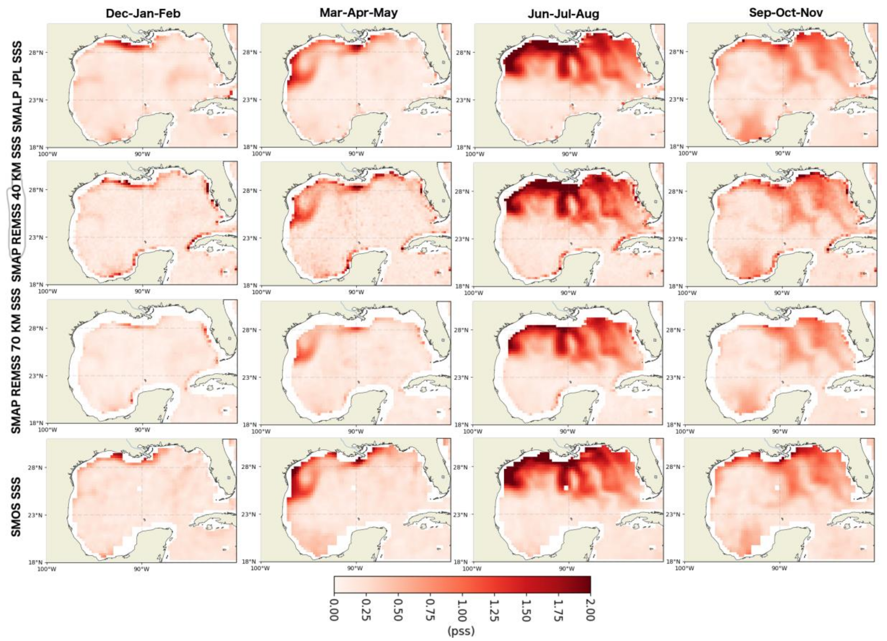
Figure 3 shows standard deviation (STD) for the seasonal means. The dominant features occur during spring through fall with a maximum variability extending offshore in summer. All four datasets show three large areas of variability, corresponding to several river plumes associated with multiple river basins, such as the Mississippi River Basin, the Mobile Bay river system basin, and the Texas river basin [28]. The largest differences are again seen closest to the coast. However, all four datasets are consistent in showing climatological variability. For example, there is a high variability in the winter in the western GoM, as well as a high variability in both summer and fall that covers much of the central and western GoM.

The remarkable consistency of the mean and STD seasonal means between the four datasets is a confirmation that, on the seasonal time scale, they are all reproducing the dominant features associated with salinity changes in the GoM, especially those associated with river discharge. Both the mean and STD establish that these datasets are consistent in reproducing climatological temporal and spatial variability, and so these datasets were further examined for possible biases and RMSD when compared with in-situ SSS from independent buoys and the WOD.

3.2. Comparisons with Buoys

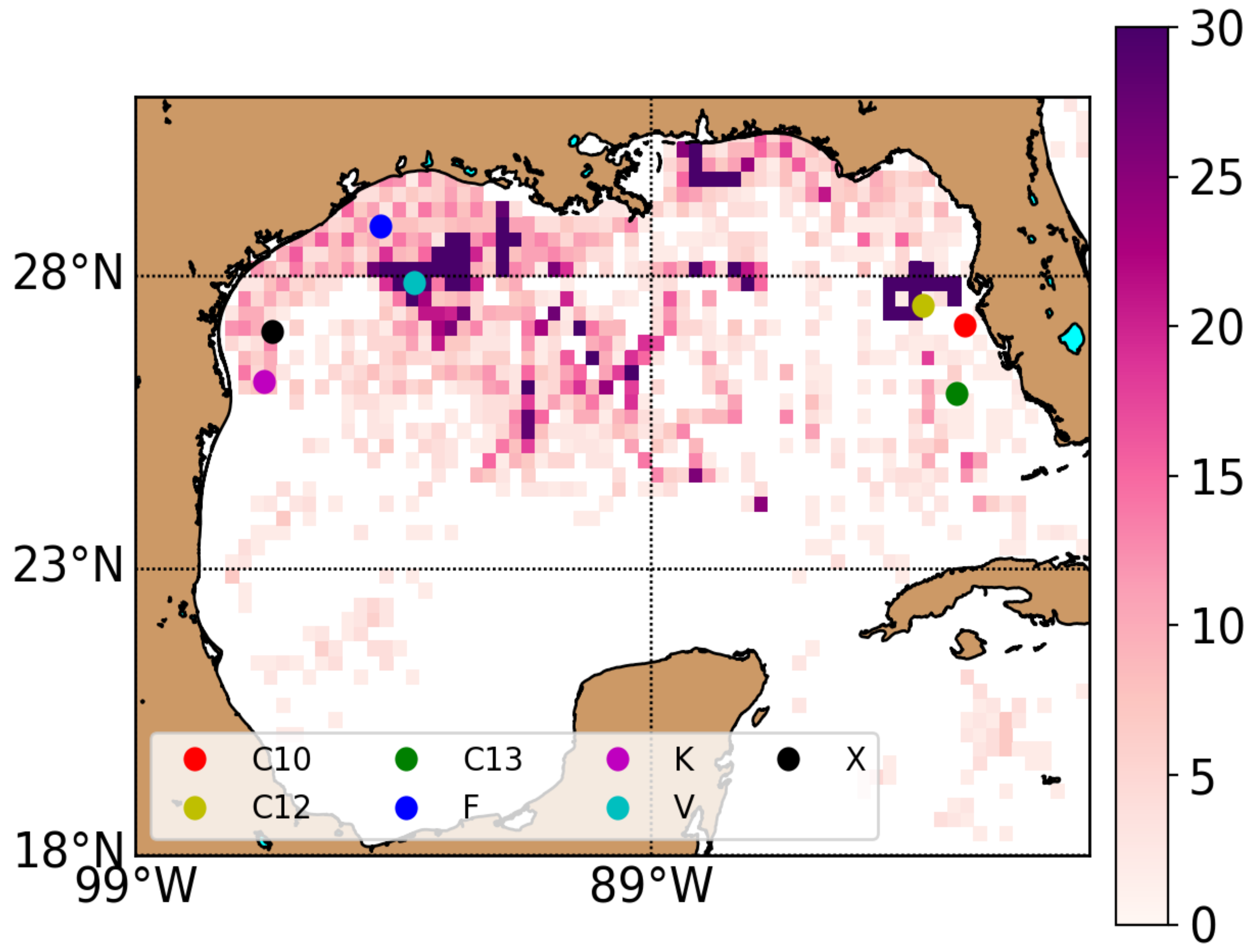
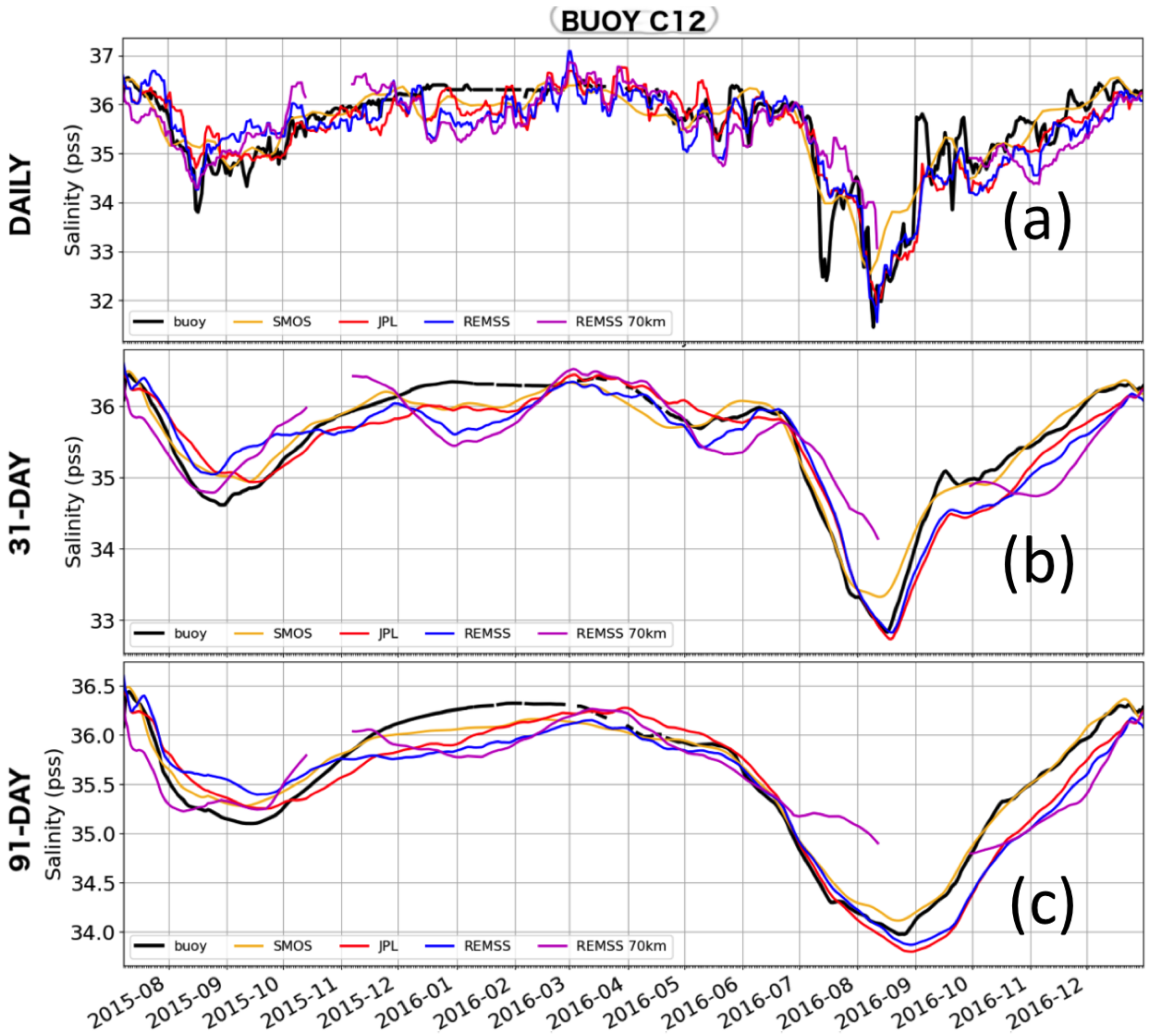
In Figure 4, Figure 5 and Figure 6, we present comparisons between satellite SSS and buoy SSS at selected buoys for three different time scales. Figure 4a–c shows the time series at buoy C12 for the 4 SSS products JPL SMAP, REMSS 40 km SMAP, REMSS 70 km SMAP, and SMOS. Figure 4 shows (a) the daily/8-day time series, (b) averaged monthly, and (c) averaged seasonally. Referencing Figure 1, buoy C12 is located approximately 100 km offshore from the west Florida coast. All the datasets show a freshening of approximately 2 pss in the summer to fall of 2016. Figure 4b,c shows similar results for smoothing at 31-day running means and 91-day running means. Results on the statistics are summarized in Table 1.

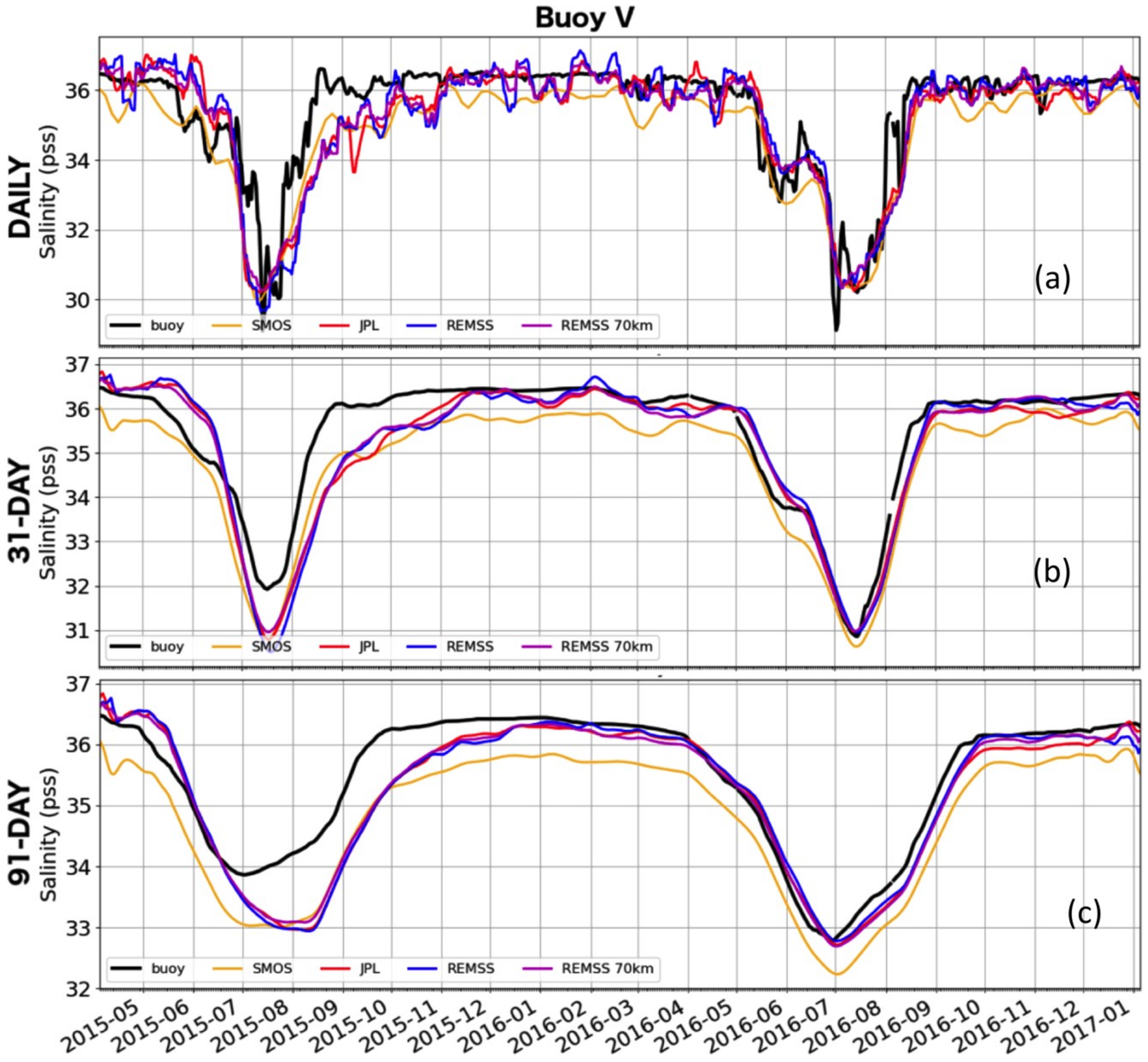
Figure 5a–c shows similar results for Buoy V, which is located approximately 400 km offshore of the Texas Coast. As with buoy C12, all four SSS datasets show the large freshening event in summer to fall of 2015 and 2016, reproducing the seasonal cycle due to river discharge [11]. Figure 5a shows the daily time series, Figure 5b the monthly means, and Figure 5c the seasonal means. The freshening seen at Buoy V of approximately 4 pss is consistent with previous reports by [11] on the extreme freshening event of 2015 associated with the flood along the Texas Coast. Similar results are shown in Figure 6a–c for Buoy F, which is located approximately 100 km from the Texas Coast. All datasets show a freshening in the summer of 2016 of approximately 5 pss.

Statistics for all the buoys are presented in Table 1. For buoy C10, it is the REMSS 40 km product that shows the best results, with fresh biases of 0.1 pss and RMSD of 0.35 at the seasonal time scale, while the JPL SMAP product has a 0.2 pss bias and a RMSD decreasing from 0.78 to 0.5 pss at seasonal time scales. Neither the REMSS 70 km product or the SMOS product have co-locations retrieved for the C10 buoy.

At buoy C12, overall SMOS shows the best results, with biases close to zero and RMSD reduced to 0.1 pss at the seasonal time scale from 0.43 pss at 9-day, similar to the JPL SMAP product. However, the JPL SMAP product shows larger fresh biases of 0.2 pss. The REMSS 40 km SMAP product has fresh biases of 0.1 pss, with RMSD reduced to 0.25 pss at the seasonal time scale from 0.5 pss. At buoy C12, the REMSS 70 km SMAP product shows slightly reduced fresh biases (approximately 0.09 pss), but the REMSS 70 km SMAP product has larger RMSD at the 8-day, monthly, and seasonal time scales (0.6, 0.5 and 0.37 pss respectively).

At buoy C13, overall SMOS has the best results, with biases close to zero, with RMSD reduced to 0.1 pss at the seasonal time scale from 0.3 pss at 9-day. The two REMSS products perform similarly, with biases close to zero and RMSD reduced to 0.25 at the seasonal time scale from 0.5 pss at 8-day. The JPL SMAP product shows fresh biases of 0.1 pss, with RMSD reduced to 0.2 pss at the seasonal time scale from 0.4 pss at 8-day.

In the western GoM, results are shown for Buoys K, F, V, and X with buoys K, F, and X being close to shore. At Buoy F, SMOS and SMAP JPL show larger salty biases of approximately 0.6 and 0.5, respectively, and similar large RMSD from 1.1 and 1.2 pss at 8 and 9-day, respectively, which reduce to 0.39 and 0.43 pss at the seasonal time scale. The REMSS 40 km SMAP product shows biases close to zero pss for the 8-day and monthly time scales, increasing to 0.1 pss at seasonal time scale. RMSD reduces from 0.9 pss at the 8-day time scale to 0.6 at the monthly time scale, before increasing to 0.89 pss at the seasonal time scale. No values are retrieved for the REMSS 70 km SMAP product, with the buoy being too close to land. Overall, the REMSS 40 km SMAP has the lowest bias whatever the time scale and the lowest RMSD at 8-day, while JPL SMAP and SMOS have lower RMSD at monthly and seasonal time scales.

At buoy K, SMOS performs better, with a fresh bias of 0.1 pss and RMSD decreasing from 1 pss at 9-day to 0.26 pss at seasonal scale. Both REMSS 40 km SMAP and JPL SMAP have biases around 0.2 pss at 8-day and monthly time scales and RMSD decreasing from 1.1 to 0.5 pss. However, while the JPL SMAP RMSD decreases to 0.4 pss at seasonal time scales, the REMSS 40 km SMAP increases to 0.6 pss. Similarly, the REMSS 70 km SMAP increases to 0.45 pss at seasonal scales from a low RMSD of 0.25 pss at monthly time scales.

At buoy V, SMOS has a large fresh bias of 0.66 pss, while JPL SMAP has an 0.4 pss fresh bias and REMSS 40 and 70 km have a fresh 0.2 pss bias. SMOS has the lowest RMSD values at every time scale, from 0.6 pss at 9-day to 0.2 pss at seasonal time scales. The three SMAP products have larger RMSD around 0.8–0.9 pss at 8-day, 0.5–0.6 at monthly and 0.4 pss at seasonal time scales.

At buoy X, the furthest offshore, SMOS shows the best results in terms of RMSD, with values of 0.24 pss at 9-day decreasing to 0.14 and 0.18 pss at monthly seasonal time scales. However, like buoys V and F, SMOS has a large fresh bias of 0.5–0.6 pss. REMSS 40 km SMAP, REMSS 70 km SMAP, and JPL SMAP products show similar results, with RMSD decreasing from 0.3–0.4 pss at 8-day to 0.25 pss at seasonal time scales. However, the REMSS SMAP product shows a bias close to zero, whereas the JPL SMAP and REMSS SMAP 70 km products show biases close to 0.2 pss.

3.3. Comparisons with the WOD

In addition to the time series, the WOD allows us to perform comparisons between satellite and in-situ SSS at many point locations, covering a large span of the GoM over different seasons. The point locations do not allow for a spatial variability study of the GoM. However, they do allow for direct comparisons with the SSS products. Figure 1 shows that the density of the WOD measurements is not sufficient to resolve the subpixel scale variability (<25 km). This type of analysis has been done by Boutin et al. [12]. Thus, interpretations of the statistics must be done considering the natural variability of the GoM. The WOD extended dataset does allow us to study the biases and RMSD of the four SSS datasets, depending on the distance from the coast or time of year or salinity range. 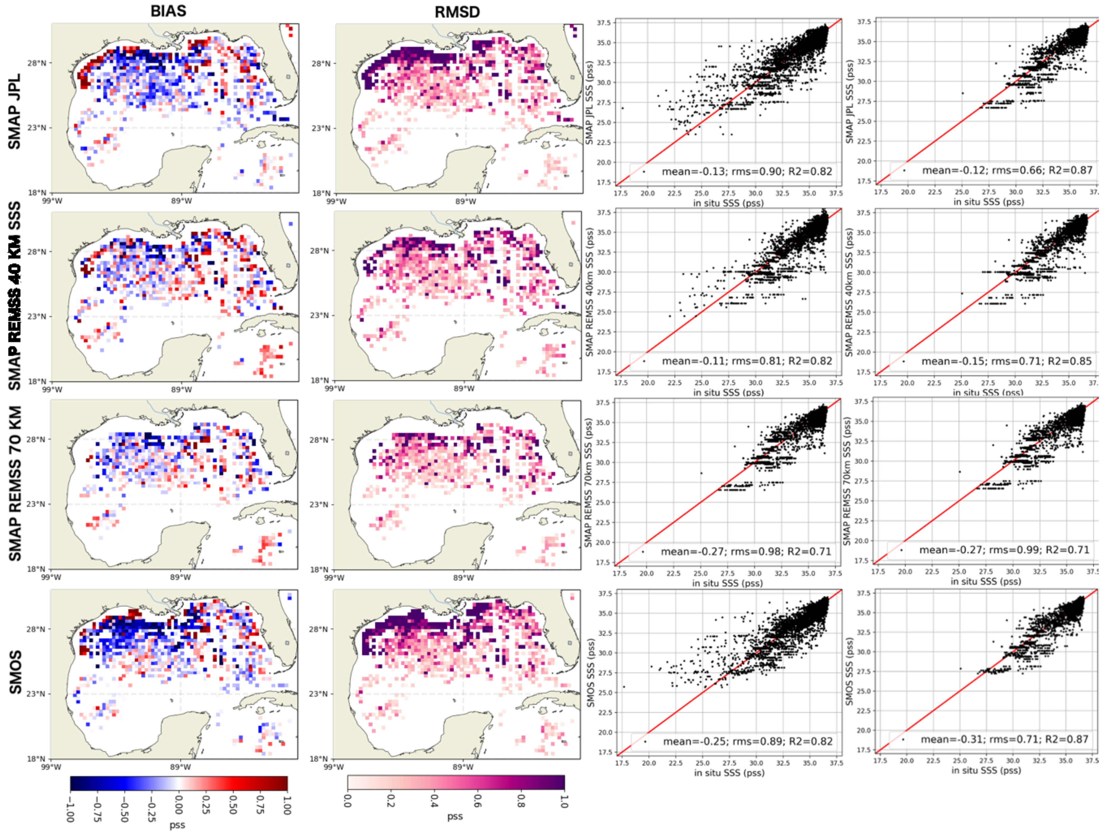Figure 7 shows the spatial distribution of the bias (first column), root mean square difference (RMSD) (second column), and scatter plots for the four SSS datasets co-located with the WOD (third and fourth columns). Overall correlations for the three products, JPL SMAP, REMSS 40 km SMAP, and SMOS had similar correlations of approximately 0.80. The REMSS 70 km SMAP product had lower correlations of 0.70. Because one cannot attribute the differences to errors due to unresolved spatial variability, the statistics have been labeled as root mean square differences (RMSD). For the WOD data comparison, there were two options available in terms of the intercomparison of multiple data sets. We chose to explore both options, namely a validation based on the temporally and spatially co-located in-situ data for each individual satellite product, as well as a validation based only on co-locations common to all of the satellite products. Thus, two scatter plots are presented: One for the analysis that takes into account the co-locations for each separate dataset (third column) and the other for the analysis based on only the common co-locations (fourth column).

Overall, when considering only the co-locations common to all datasets, RMSD values are very similar across the datasets, with a value of 0.7 for REMSS 40 km SMAP, JPL SMAP, and SMOS and 0.99 for REMSS 70 km SMAP. The bias is larger for SMOS (0.3 pss), whereas it is lower for REMSS 70 km SMAP (0.27 pss), JPL SMAP (0.25 pss), and REMSS 40 km SMAP (0.15 pss), biases being fresher in all cases. When considering all the co-locations possible for each individual dataset, the RMSD increases to 0.9 for JPL SMAP and SMOS, and to 0.8 for REMSS 40 km SMAP. The fresh biases also decrease to 0.25 for SMOS and JPL SMAP and 0.11 for REMSS 40 km SMAP. An interesting feature is the difference in the statistics based on using all the co-locations and only those common to all the products. This indicates that the major differences in the statistics (confirmed later) are occurring close to land where the dominant differences in the number of co-locations are found. Additionally, the lower correlations for the SMAP 70 km product are most likely reflective of the smoother product not resolving mesoscale and submesoscale variability associated with the Gulf of Mexico. Overall, the JPL SMAP and SMOS products had the highest correlation. This will also be discussed later in the context of the signal to noise ratio.

The top panels of Figure 7 show the bias, RMSD, and scatter plots for the JPL SMAP product. Overall, the largest biases and differences are seen close to shore. Nearshore biases reach 1 pss, with the JPL SMAP product being saltier than the WOD. RMSD reaches 1 pss in the nearshore area. The second and third panels from the top show the statistics for the REMSS 40 km SMAP and REMSS 70 km SMAP products, respectively. The same general trend exists with saltier biases and larger RMSD near the coast. In the spatial distribution plots, one notices that the 70 km product lacks values nearer to the coast than those of the REMSS 40 km SMAP or JPL SMAP products. A reason for the possible differences in the biases between the 40 km and 70 km product is most likely a combination of both the mesoscale variability in the GoM and the REMSS 40 km SMAP product resolving features closer to land. The bottom panel shows the statistics for the SMOS product. SMOS data show large negative biases (1 pss) along the coast, consistent with the large RMSD in the other SMAP datasets. However, SMOS data show slightly more values closer to the coast. RMSD are also greater than 1 pss close to the coast.

The selection of only the co-located values common to all of the datasets generally impacts the RMSD, which decreases to approximately 0.7 pss from the individual comparisons, mostly due to the elimination of stations within 70 km of the coast. The results (which will be discussed in the next section) appear to indicate that the largest discrepancies across satellite data products appear close to land or at low salinity during summer (when the region is mostly influenced by riverine waters). To fully understand the impact of the distance from land on the statistics, the next step was to derive the statistics from the WOD based on distance to land, salinity values, and period of the year. In the GoM, as in other regional basins, assessing the quality of the SSS near to land is critical for quantifying the effects of river discharge on seasonal to interannual time scales.

Summarizing, three major contributors to the differences between the SSS products and in-situ data may be evaluated based on the comparisons of the satellite products with the buoys and the WOD SSS: (1) How different do the four SSS products behave close to land? (2) Are there seasonal or discharge event effects on product performance? (3) What is the impact of faster time-scale processes on apparent error in salinity products? These questions address critical information needed for understanding SSS applications for coastal processes and dynamics. Here we highlight key differences between the four products, with the goal of helping future science users to better understand the existing SSS products. To address these questions, one needs to examine in more detail the four SSS products and their relationship to the WOD and buoy data. The Discussion section will address the three above issues.

4. Discussion

4.1. Impact of Distance from Land on Differences

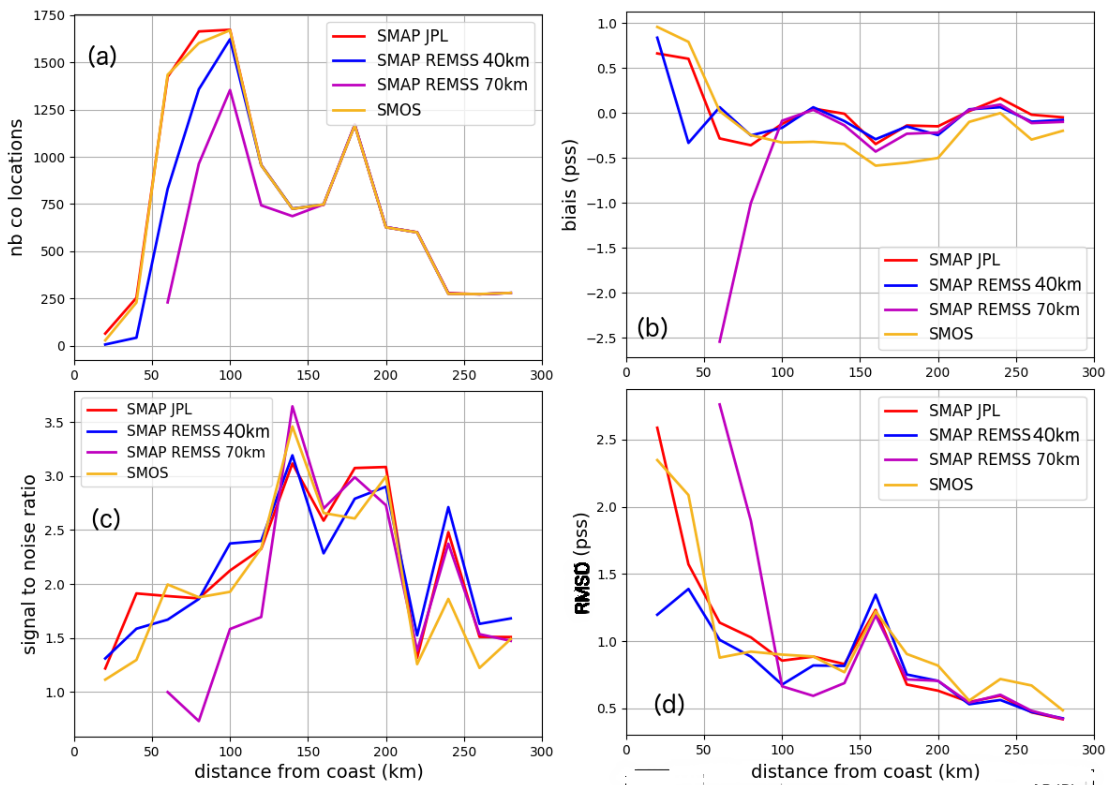
We quantify the dependence of bias and RMSD of the four SSS products with respect to distance from shore (Figure 8). The top left panel (Figure 8a) shows the number of co-locations for each of the products. As expected, the REMSS 70 km SMAP product has the fewest number of co-locations. Additionally, the 70 km product does not retrieve values closer to land than 70 km, consistent with the spatial distribution maps. SMOS and SMAP JPL have the maximum number of co-locations within the first 100 km, while REMSS 40 km SMAP has fewer co-locations, suggesting that there are fewer product data near the coast. The maximum number of co-locations occurs at approximately 100 km from shore, decreasing in both the shoreward and offshore directions. At distances greater than 100 km from shore, the JPL SMAP, REMSS 40 km SMAP, and SMOS converge on the number of co-locations. This is consistent with the decreasing influence of land contamination on the three different products. Additionally, it shows that a large percentage of the WOD is concentrated close to land, consistent with Figure 7.

Figure 8b, the top right panel, shows the bias as a function of distance from shore for the four SSS products. All the products, for distances less than 100 km, show increasing biases. For JPL SMAP, REMSS 40 km SMAP, and SMOS, saltier biases occur close to land, indicating the satellite-based products are saltier than the WOD, which is consistent with what is seen on the scatter plots in Figure 7. SMOS has biases that increase to 1 pss near the coast (based on location of in-situ data). The JPL SMAP and REMSS 40 km products overall have smaller biases, approximately 0.6 and 0.7 pss. The REMSS 70 km SMAP product, however, shows large fresh biases, reaching 2.5 pss within 70 km from shore. Negative biases would be consistent with possible land contamination. However, an explanation for this is beyond the scope of this article, but should be explored in future work. For distances greater than 100 km from the coast, all four products converge to fresh biases of less than 0.5 pss. The change in the statistics at 100 km is very similar to results found by Fournier et al. [10].

Figure 8c shows the signal to noise ratio as a function of distance from the coast. For all four products, the signal to noise ratio reaches a maximum of approximately 3–3.5 at 140 km from shore, decreasing to 1–2 closer to shore for SMOS, JPL SMAP, and REMSS 40 km SMAP. The REMSS 70 km SMAP product shows the smallest signal to noise ratio of less than 1 within the first 100 km. At less than 70 km, the JPL SMAP and SMOS products have the largest signal to noise ratios. SMOS has the largest signal to noise of approximately 2.0 at distances less than 100km while the JPL SMAP has a signal to noise ratio of approximately 1.5.

Figure 8d shows the RMSD as a function of distance from shore. Close to shore, less than 100 km, the REMSS 40 km SMAP has maximum values of 1.4 pss, whereas SMOS and JPL SMAP have significantly larger RMSD values of 0.9–2.5 pss. From 50 km and further, the RMSD values of SMAP JPL, REMSS 40 km SMAP, and SMOS converge. REMSS 70 km SMAP, however, has larger RMSD values up to 100 km from the coast, reaching 2.7 pss at around 70 km. At distances greater than 100 km, all four products converge to values between 0.5 pss and 1.0 pss. Thus, comparing the RMSD with the signal to noise ratio indicates that the larger SMOS and JPL SMAP signal to noise ratios are likely due to larger STD values of the individual products and ability of the SMOS and JPL SMAP to resolve features closer to land. This is also consistent with the JPL SMAP and SMOS having the overall highest correlations.

Considering the comparisons of satellite SSS to the in-situ SSS from the buoys (statistics presented in Table 1), the buoys that are closest to shore (buoys C10, K, F, and X) show the largest biases and RMSD. REMSS 40 km SMAP has the lowest RMSD values (0.6 pss) at buoys C10, the closest to shore, while neither SMOS nor REMSS 70 km SMAP retrieve data. At buoys K and X, SMOS has the lowest RMSD values of 1 and 0.24 pss, respectively. However, at buoy X, SMOS has the largest bias, which is consistent with Figure 8b. On the Florida shelf, buoy C12 is further from the coast and showed improved statistics over buoy C10 for every product. Similarly, on the Texas shelf, buoy V, further offshore than buoy F, shows improvements in biases and RMSD values for all the products.

Overall, all three JPL SMAP, REMSS 40 km SMAP, and SMOS products behave comparably as a function of the distance from the coast, with larger biases and RMSD closer to the coast and lower signal to noise ratios. SMOS has, however, the largest bias closer to the coast, while REMSS 40 km SMAP has a lower RMSD value. At some locations, SMOS has lower RMSD values, even close to the coast, as shown by comparisons with buoys. All four products have a maximum in the signal to noise ratio at approximately 150 km from shore.

4.2. Impact of Riverine Freshwater on Differences

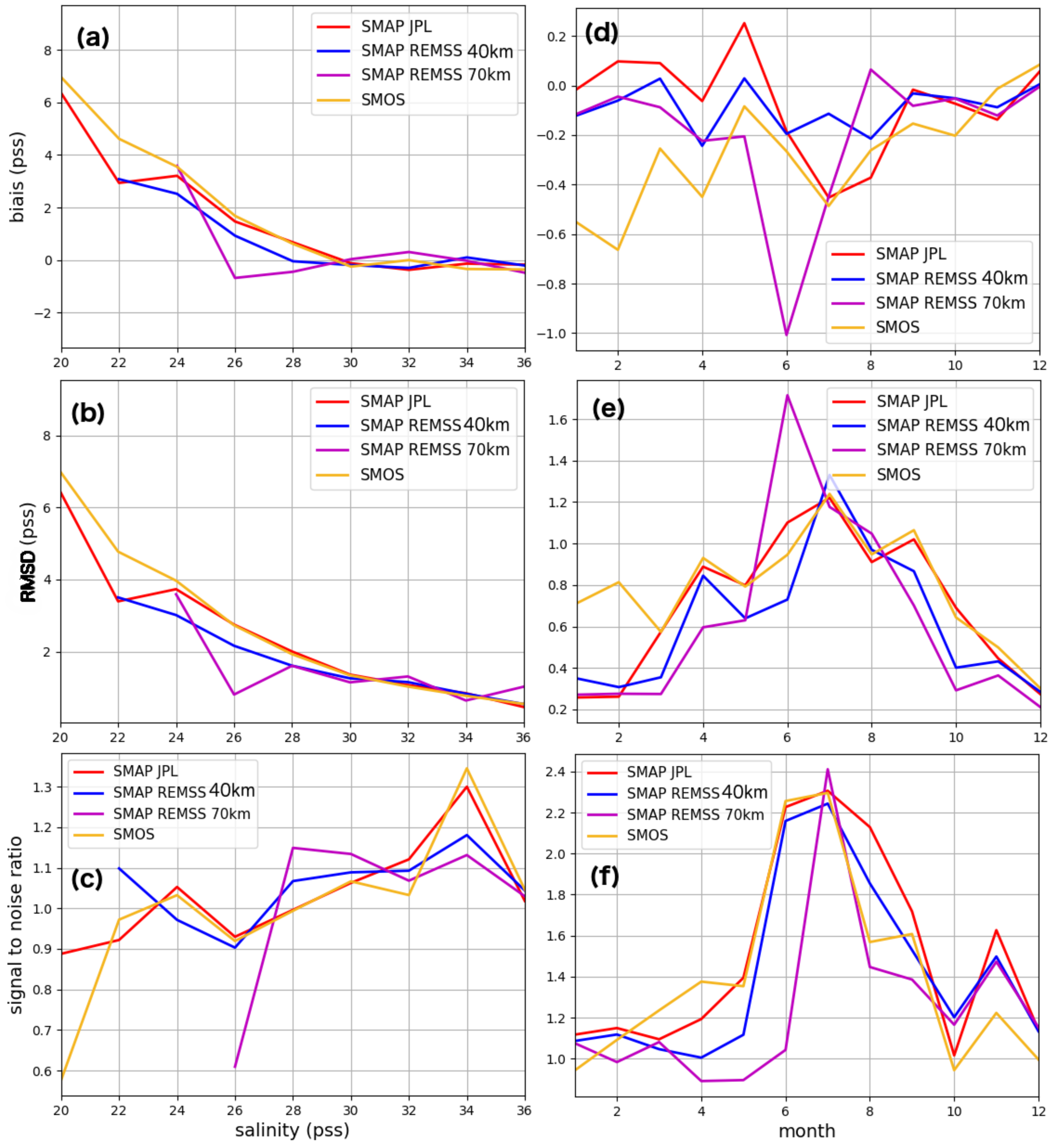
A remaining question is how the errors might be related to riverine freshwater discharge into the GoM. Figure 9 shows the statistics based on the same datasets used as Figure 8, but as a function of salinity (first column) and time of year (second column). Figure 9 confirms what is shown in Figure 8, which is that REMSS 40 and 70 km do not capture the lowest salinity near the coast. While REMSS 40 km SMAP does not capture any salinity lower than 22 pss (20 pss for JPL SMAP and SMOS), REMSS 70 km SMAP only captures salinity higher than 26 pss. Because a majority of the WOD database in the area are CTDs, point measurements, an analysis of the spatial variability is not feasible and beyond the scope of the work. Future work, incorporating new measurements, would help to quantify the differences that are due to the spatial variability of the GoM.

From Figure 9a, all four products show significant saltier biases of greater than 2 pss for salinity values less than 25 pss and can reach as high as 6–7 pss. For salinity values greater than 26 pss, biases are reduced to near 0 pss. Figure 9d shows the bias as a function of the time of year, May to September being the period of time after the maximum Mississippi River discharge. Overall, the JPL SMAP and REMSS 40 km show no significant differences based on time of year, with biases of less than 0.2 pss. SMOS tends to exhibit a larger bias in winter from January to April (−0.6 in January and February against −0.1 to 0.1 for the other three products). The REMSS 70 km SMAP product has a significant large fresh bias of 1 pss during the summer time frame (when the region is impacted by riverine fresh water). One possible explanation is that the smoother resolution is not fully resolving the spatial scales of the discharge. A more detailed explanation needs to be examined in future work.

Figure 9b shows the same results for the RMSD. For salinity values less than 25 pss, RMSD values increase rapidly to greater than 3 pss (reaching 6–7 pss), with RMSD being slightly lower for the REMSS 40 km SMAP product than for the others. Figure 9e shows that the REMSS 70 km SMAP product has a maximum RMSD of greater than 1.6 pss in June, while the other three products reach maxima of 1.2 pss in July. Thus, all four products show maxima in RMSD during seasonal maxima in freshwater discharge. Large biases in the REMSS 70 km SMAP in June are also consistent with a maximum in the RMSD. Here, the RMSD values are also slightly lower for REMSS 40 km SMAP all year long except in June, during the peak RMSD value.

Figure 9c,f shows similar results, but for the signal to noise ratio. There is a slight trend of increasing signal to noise ratio with increasing salinity for the three products, JPL SMAP, REMSS 40 km SMAP, and SMOS. The REMSS 70 km SMAP shows a sharp minimum of 0.6 signal to noise ratio at 25 pss and has, overall, a lower signal to noise ratio all year long. All four products show a shared maximum of 2.4 in the signal to noise ratio in July.

Overall, all the products indicate that RMSD, biases, and signal to noise ratio depend on the salinity values and time of year. Large freshwater biases, large RMSD, and lower signal to noise ratio occur in the summer time frame, when the area is affected by riverine freshwater. While JPL SMAP, REMSS 40 km SMAP, and SMOS have comparable results, the REMSS 70 km SMAP product has larger biases and RMSD associated with the summertime freshwater river discharge.

4.3. Impact of Temporal Sampling on Differences

Because co-located satellite and in-situ observations may not truly be co-located at a precise spatial point and may also have different sampling frequencies, it is possible that the undersampling of high-frequency variability in either data source may lead to a type of “aliasing” noise, which decreases the skill of a specific validation. While we are limited in the format of the available data, we can look more closely at the possible temporal effects on our results. These effects could indicate results or trends in validation that may be influenced by forces commonly referred to as “luck”. As such, we examine temporally smoothed results to check for consistency and to examine the gross behavior of the products and their ability to capture major dominant signals. Overall, interpreting the smoothing impact on the statistics is critical for understanding the possible impacts of spatial variability on the statistics. This is especially true in the GoM, where mesoscale and sub-mesoscale variability can dominate during the formation of the loop current and associated eddy detachments.

Table 1 summarizes the comparison statistics of the JPL SMAP, REMSS 40 km SMAP, REMSS 70 km SMAP, and SMOS with the 7 buoys at three different time scales. Overall, with temporal smoothing from 8/9-day to monthly to seasonal time scales, there is a significant improvement in the RMSD for all the products. On average, at 8/9-day across products, the RMSD is about 0.7 pss, whereas it decreases to 0.4 at monthly and 0.3 at seasonal time scales.

From 8/9-day to monthly time scales, the improvement in RMSD extends across products, with a decrease of 0.1 reaching 1 pss, with an average of 0.28 pss. The largest improvements are seen at buoys F and K near shore on the Texas shelf, with a decrease of 1 pss for REMSS 70 km, 0.7 pss for SMOS, 0.6 pss for REMSS 40 km SMAP, and 0.55 pss for JPL SMAP at buoy K. JPL SMAP RMSD improves, with a decrease of 0.65 pss at buoy F, and SMOS RMSD with a decrease of 0.5 pss. From monthly to seasonal time scales, the improvement in RMSD is lower, with a decrease of 0.05 to 0.3 pss and an average of 0.1 pss. However, for the REMSS 40 and 70 km, there is an increase in the RMSD of 0.3 pss at buoy F and 0.1 pss at buoy K for REMSS 40 km SMAP and an increase of 0.2 pss at buoy K for REMSS 70 km. Consistent improvement also occurred with respect to correlations in going from the 8-day to seasonal time scale, indicative of the reduction in noise. The overall trend shows the JPL SMAP and SMOS products had the highest correlations. The SMOS product showed a correlation of 0.98 at Buoy V (furthest offshore) for the seasonal time scale. REMSS 70 km SMAP had negative correlations (consistent with the large negative biases near land) at Buoy X.

5. Conclusions

This work examines the performance of several satellite SSS products in a representative marine system that is significantly impacted by river discharge. The comparisons of four satellite derived SSS products (REMSS 40 km SMAP, REMSS 70 km SMAP, JPL SMAP, and SMOS) in the GoM demonstrate that these products generally perform well compared to in-situ observations in a basin that has large temporal and spatial variability in the surface salinity structure. In interpreting the results, it is important to consider not only how the differences between the satellite products and in-situ data affect the correlations and signal to noise ratio, but also how the inherent spatial variability of the GoM might not be resolved by the individual products, depending on smoothing. The remarkable consistency of the seasonal mean and STD between the four datasets confirms that, on the seasonal time scales, they are all reproducing the dominant features associated with salinity changes in the GoM, especially those associated with river discharge.

The satellite datasets were compared with buoys salinity data on the Florida and Texas shelves and with a large amount of diverse in-situ measurements from the WOD. We computed biases, RMSD, and signal to noise ratio to address three issues: (1) The impact of distance from shore, (2) the impact of freshwater river discharge, and (3) the impact of temporal variability.

Overall, JPL SMAP, REMSS 40 km SMAP, and SMOS products are comparable, independent of distance from the coast, when compared with WOD in-situ data. Within the first 100 km from the coast, the three products showed increasing biases and RMSD and a decrease in the signal to noise ratio towards the shore. Saltier biases close to shore are likely due to some residual land contamination and possible overestimation of the land correction. Additional error arises due to the fact that, closer to the coast, larger horizontal and vertical salinity gradients can be observed, altering the comparison between a 40 to 70 km satellite footprint with a point-location from an in-situ measurement. These three products exhibit a similar low signal to noise ratio close to shore that peaks at 150 km from the coast. They also show a larger RMSD within the first 100 km from the coast, before decreasing to 0.5–1.5 pss further than 100 km.

Even if the products behave similarly overall, some differences can be observed between the products near the coast. The REMSS 40 km SMAP product shows the lowest bias overall (−0.15 pss against −0.25 for JPL SMAP and −0.31 for SMOS). It also shows the lowest RMSD (1.2 to 1.4 pss) within the first 60 km, while the SMOS and JPL SMAP product show a RMSD of 1.5 to 2.5 pss. However, REMSS 40 km SMAP retrieves fewer data closer to the coast than JPL SMAP and SMOS do and may not support an equivalent comparison. This might be due to more stringent land corrections applied.

The SMOS product exhibits the largest RMSD values near the coast and at low salinities. It also exhibits the largest bias overall (−0.31 pss), especially at low salinity and during winter independent of the distance from the coast. However, our results on the comparisons with buoys suggest that at some locations, even near the coast, SMOS has the lowest RMSD values of all of the products. However, at buoys on the Texas shelf, SMOS exhibits the largest bias, reaching 0.7 pss against a bias of 0 to 0.4 for the other products. These results are important to consider in light of the fact that the SMOS product provides the longest satellite SSS record currently available. The JPL SMAP product gets similar results to the SMOS product when compared with the WOD, especially near the coast. However, SMAP JPL doesn’t exhibit large bias values (−0.25 overall versus −0.31 for SMOS).

Because of the required spatial smoothing, the REMSS 70 km SMAP product does not offer any data within 70 km of the coast, reducing its usefulness in coastal applications. Moreover, within the first 100 km of the coast, this product exhibits a much larger bias, reaching −2.5 pss. It also exhibits a lower signal to noise ratio within the first 140 km of the coast and a higher RMSD value. Results are consistent with assumed error characteristics based on the smoothness of the REMSS 70 km SMAP product that reduces accuracy close to land.

Temporal variability demonstrates a clear effect on error characteristics across the products. At seven buoys located in the eastern and western GoM, smoothing over the 8/9-day to seasonal time scales decreased the RMSD significantly, with an average RMSD at 8/9-day across the product of 0.7 pss, 0.4 pss at monthly, and 0.3 pss at seasonal time scales. While temporal sampling is clearly a factor for each of the products tested, the validation results described above hold and are consistent in terms of which products perform best even after temporal smoothing is applied, with performance generally improved at longer timescales.

Because of the number of SSS products now available, the goal of this study was to present a validation in a coastal region based on independent in-situ data. The results are presented here in a format that we hope will give the users an overall assessment of what datasets are best for different applications in the GoM. Generally, close to land (less than 100 km), the REMSS 40 km SMAP product performs well and exhibits the smallest RMSD values. However, it has fewer co-locations, suggesting that there are fewer product data near the coast, likely due to some filtering of lower quality, nearshore observations. Additionally, at some specific locations, when compared with buoys, SMOS shows lower RMSD values whatever the distance from the coast. JPL SMAP and SMOS have similar overall RMSD values near the coast, with JPL SMAP having a much lower bias value.

The broadening of the footprint of in-situ ocean observing systems, as well as the increased archival efforts required by many funding agencies, is increasing the availability of data, and we hope this work can serve as a template for other such regional comparisons in a coastal, semi-enclosed basin. Future work should focus on applying similar methodologies to other regions, while taking advantage of coastal datasets.