Long-Term Surface Water Dynamics Analysis Based on Landsat Imagery and the Google Earth Engine Platform: A Case Study in the Middle Yangtze River Basin


Abstract
:1. Introduction
2. Materials and Methods
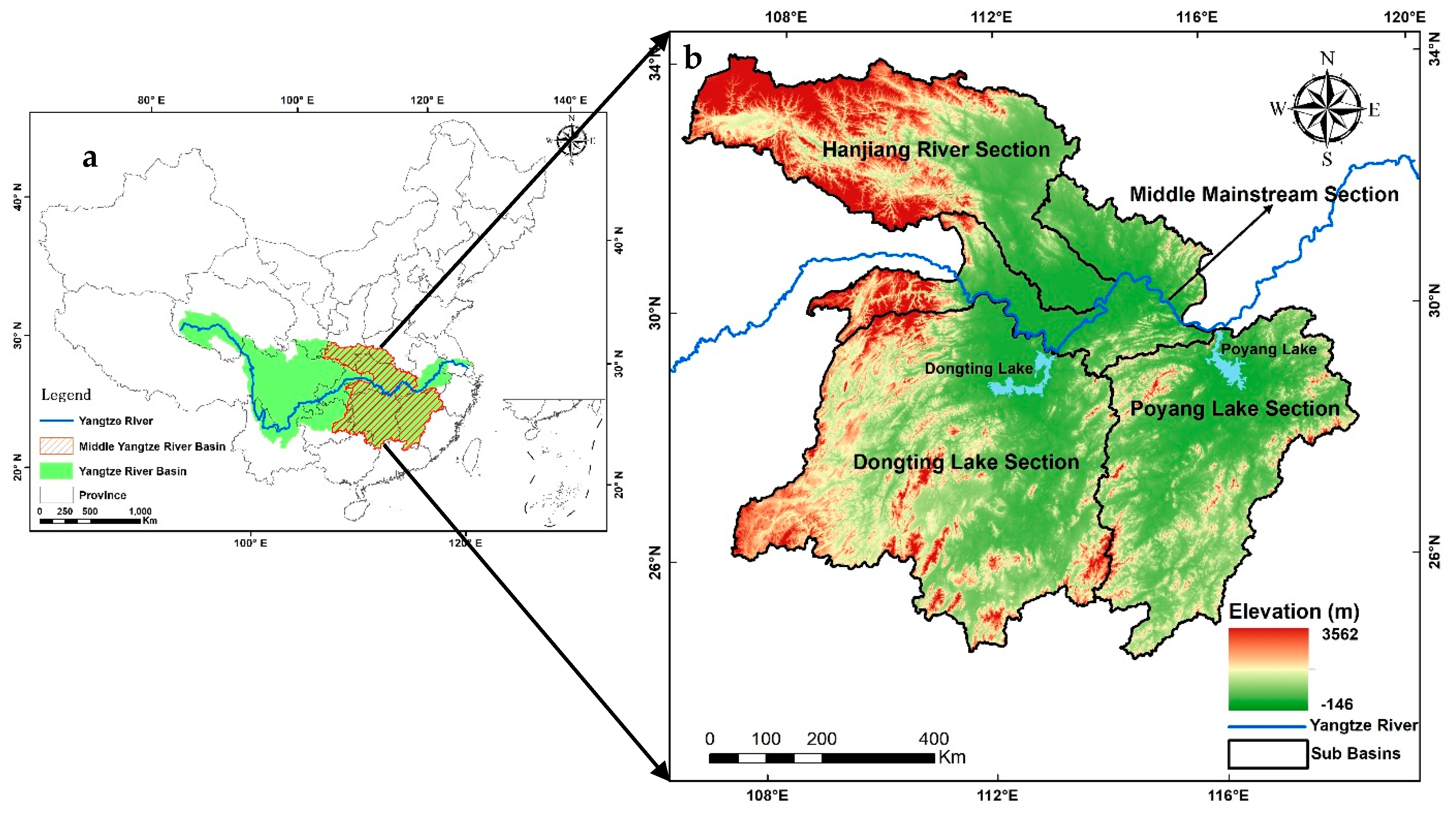
2.1. Study Area
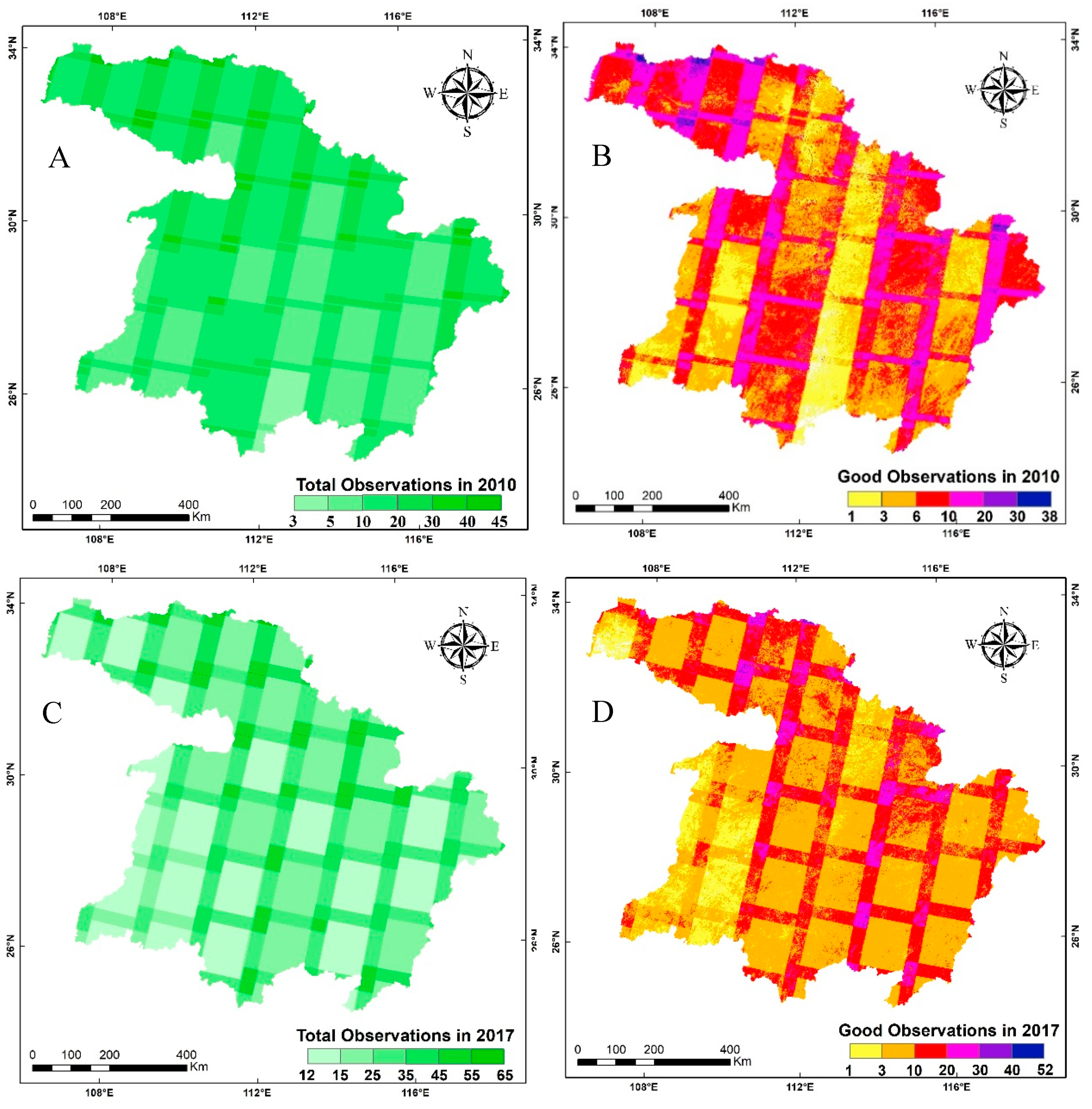
2.2. Data Preparation
2.3. Methodology
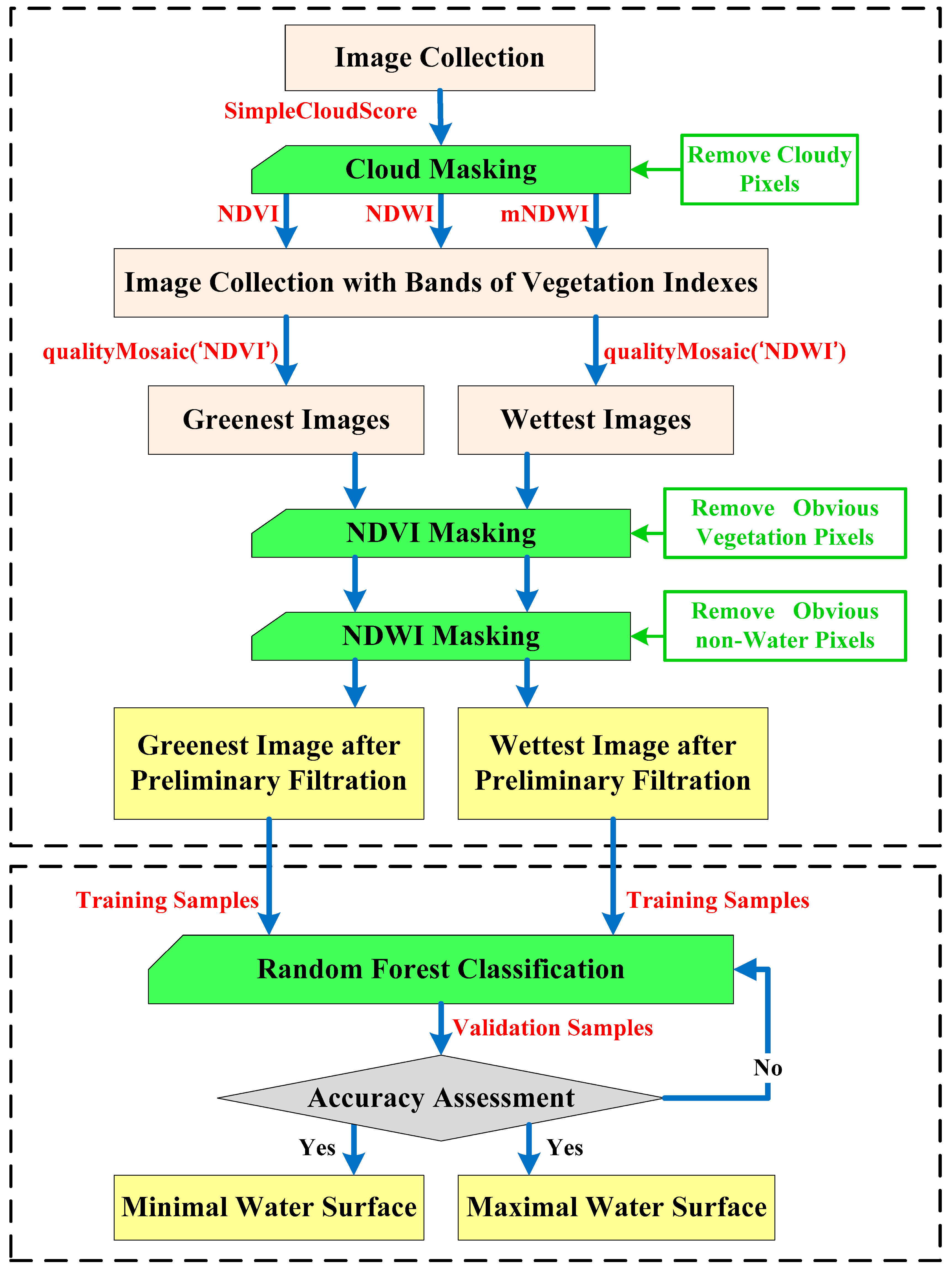
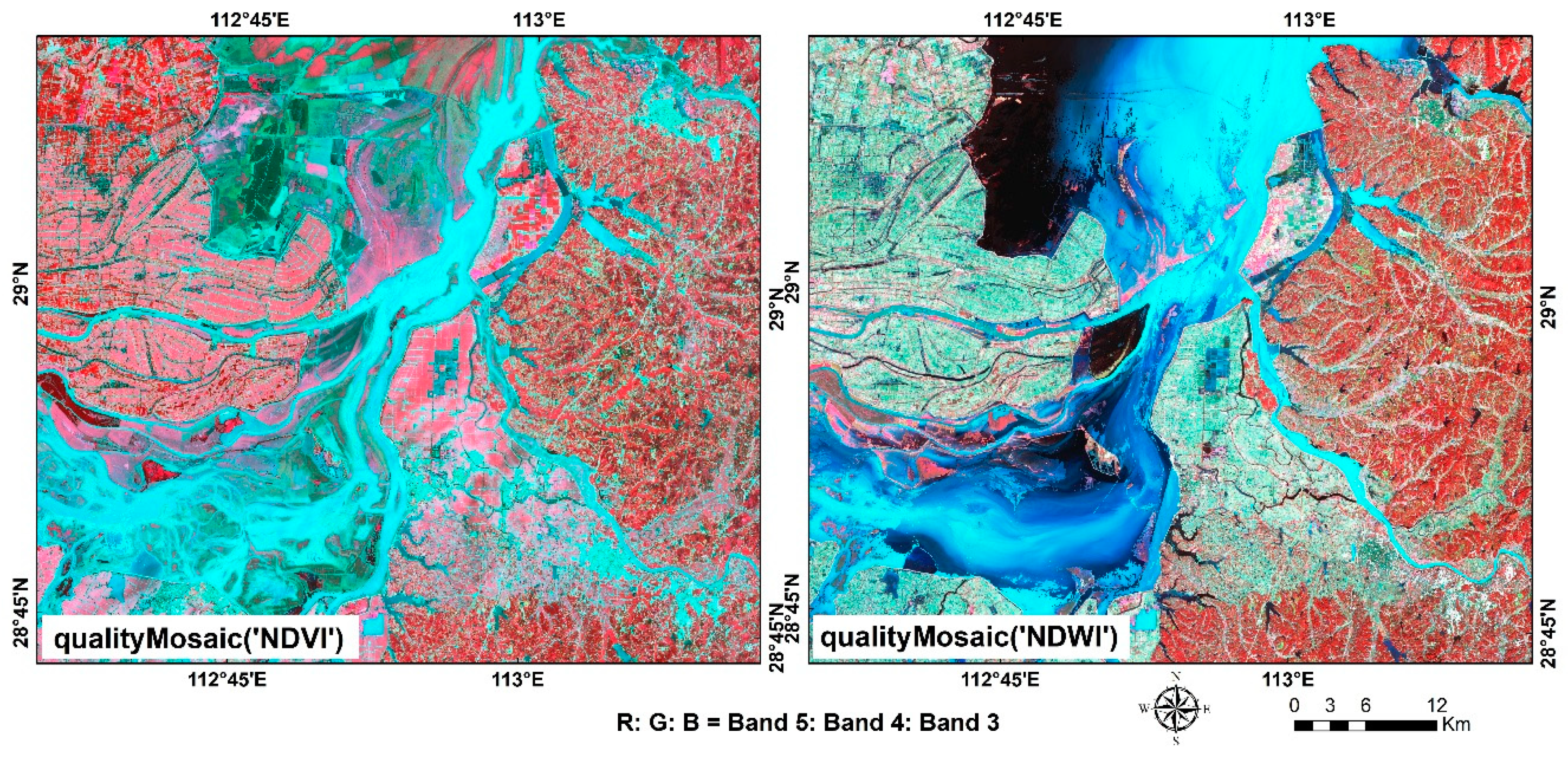
2.3.1. Removing Obvious Non-Water Pixels by Normalized Difference Indexes
2.3.2. Further Extracting Surface Water Pixels by Random Forest (RF)
3. Results
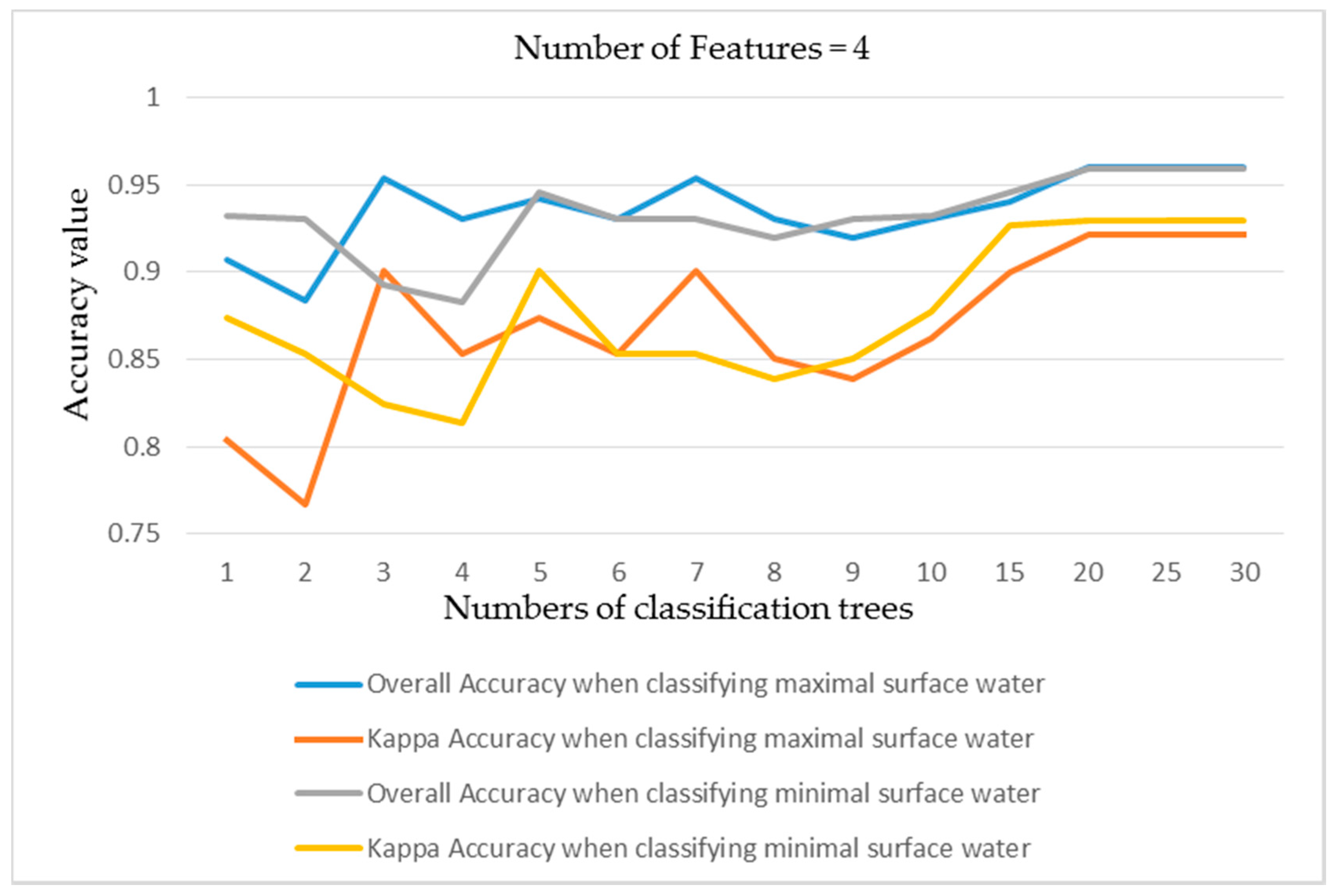
3.1. Accuracy Assessment
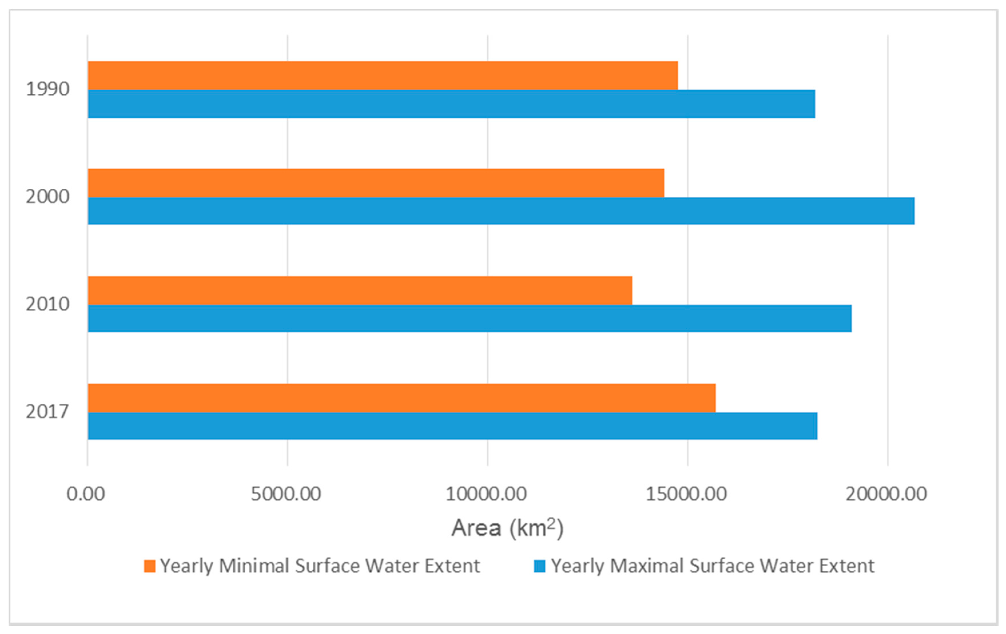
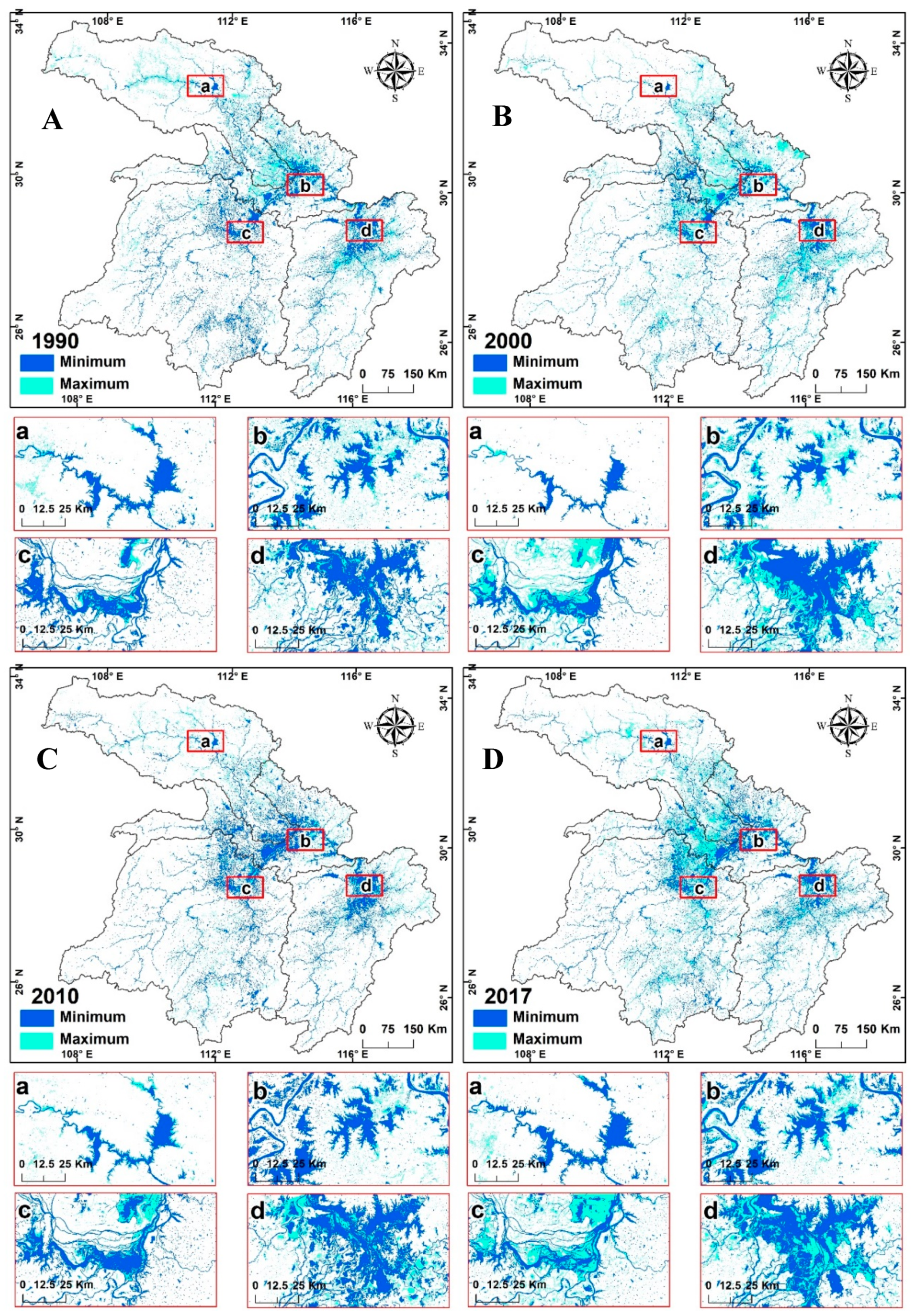
3.2. Area and Distrubution of Surface Water in the MYRB from 1990 to 2017
4. Discussion
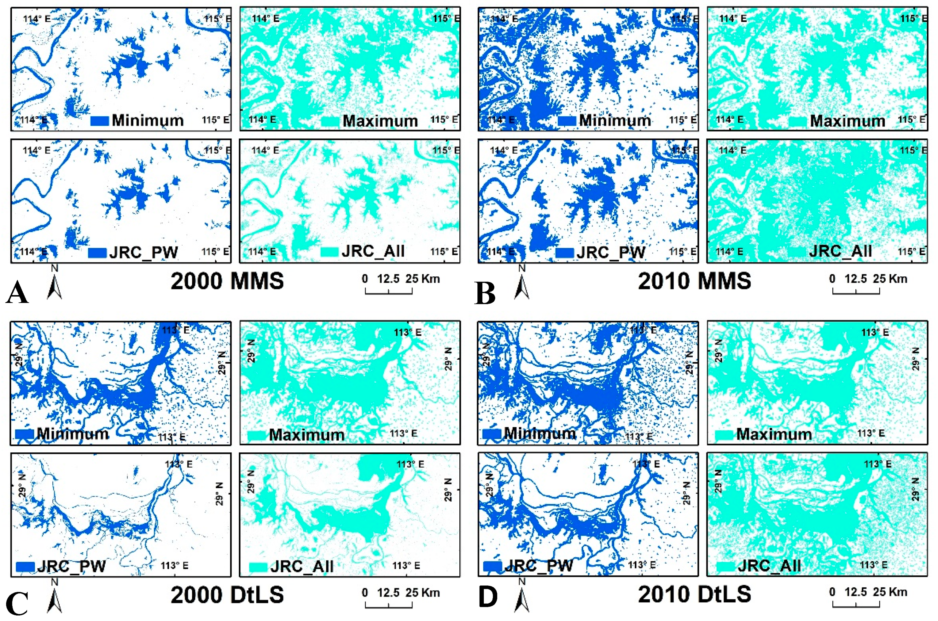
4.1. Comparison with JRC Yearly Water Classification History
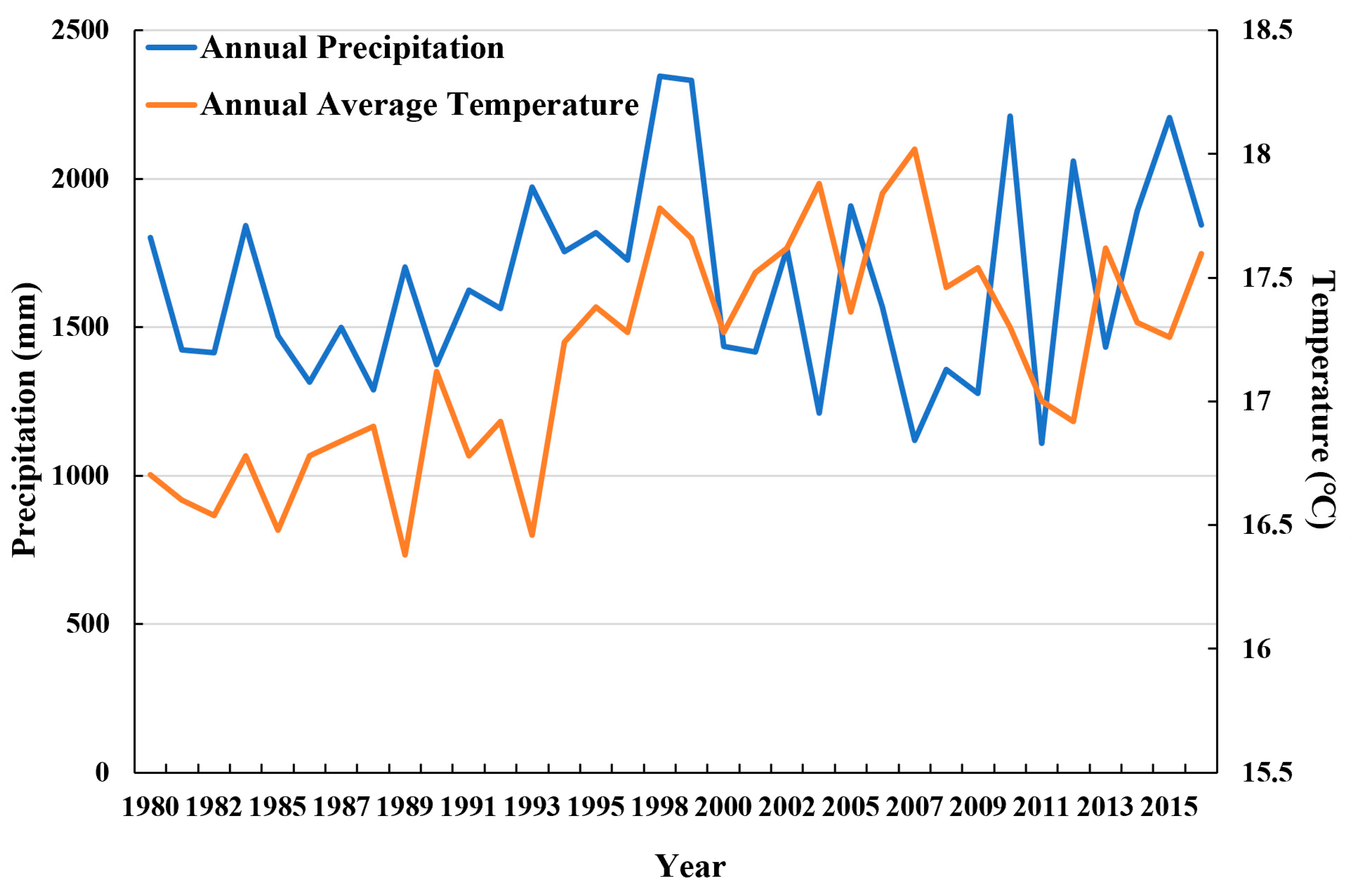
4.2. Surface Water Changes Influenced by Natural and Human Factors
4.3. Advantages and Limitations of Using GEE
5. Conclusions
Supplementary Materials
Author Contributions
Funding
Acknowledgments
Conflicts of Interest
References
- United Nations Educational, Scientific and Cultural Organization. The UN World Water Development Report 2015, Water for a Sustainable World. Available online: http://www.unesco.org/new/en/natural-sciences/environment/water/wwap/wwdr/2015-water-for-a-sustainable-world/ (accessed on 19 July 2018).
- Carroll, M.; Wooten, M.; DiMiceli, C.; Sohlberg, R.; Kelly, M. Quantifying surface water dynamics at 30 m spatial resolution in the north american high northern latitudes 1991–2011. Remote Sens. 2016, 8, 622. [Google Scholar] [CrossRef]
- Goldblatt, R.; You, W.; Hanson, G.; Khandelwal, A.K. Detecting the boundaries of urban areas in india: A dataset for pixel-based image classification in google earth engine. Remote Sens. 2016, 8, 634. [Google Scholar] [CrossRef]
- Koning, C.O. Vegetation patterns resulting from spatial and temporal variability in hydrology, soils, and trampling in an isolated basin marsh, new hampshire, USA. Wetlands 2005, 25, 239–251. [Google Scholar] [CrossRef]
- Robledano, F.; Esteve, M.A.; Farinós, P.; Carreño, M.F.; Martínez-Fernández, J. Terrestrial birds as indicators of agricultural-induced changes and associated loss in conservation value of mediterranean wetlands. Ecol. Indic. 2010, 10, 274–286. [Google Scholar] [CrossRef]
- Pekel, J.-F.; Cottam, A.; Gorelick, N.; Belward, A.S. High-resolution mapping of global surface water and its long-term changes. Nature 2016, 540, 418–422. [Google Scholar] [CrossRef] [PubMed]
- Li, L.; Vrieling, A.; Skidmore, A.; Wang, T.; Turak, E. Monitoring the dynamics of surface water fraction from modis time series in a mediterranean environment. Int. J. Appl. Earth Obs. Geoinf. 2018, 66, 135–145. [Google Scholar] [CrossRef]
- Colwell, R.N. Remote sensing of natural resources. Sci. Am. 1968, 218, 54–71. [Google Scholar] [CrossRef]
- Planet, W.G. Some comments on reflectance measurements of wet soils. Remote Sens. Environ. 1970, 1, 127–129. [Google Scholar] [CrossRef]
- Sharma, K.; Singh, S.; Singh, N.; Kalla, A. Role of satellite remote sensing for monitoring of surface water resources in an arid environment. Hydrol. Sci. J. 1989, 34, 531–537. [Google Scholar] [CrossRef] [Green Version]
- Chahine, M.T. The hydrological cycle and its influence on climate. Nature 1992, 359, 373. [Google Scholar] [CrossRef]
- Gillies, R.R.; Carlson, T.N. Thermal remote sensing of surface soil water content with partial vegetation cover for incorporation into climate models. J. Appl. Meteorol. 1995, 34, 745–756. [Google Scholar] [CrossRef]
- Mattikalli, N.M.; Richards, K.S. Estimation of surface water quality changes in response to land use change: Application of the export coefficient model using remote sensing and geographical information system. J. Environ. Manag. 1996, 48, 263–282. [Google Scholar] [CrossRef]
- Kite, G.; Pietroniro, A. Remote sensing of surface water. In Remote Sensing in Hydrology and Water Management; Springer: Berlin, Germany, 2000; pp. 217–238. [Google Scholar]
- Alsdorf, D.E. Water storage of the central amazon floodplain measured with gis and remote sensing imagery. Ann. Assoc. Am. Geogr. 2003, 93, 55–66. [Google Scholar] [CrossRef]
- McFeeters, S.K. The use of the normalized difference water index (ndwi) in the delineation of open water features. Int. J. Remote Sens. 1996, 17, 1425–1432. [Google Scholar] [CrossRef]
- Han-Qiu, X. A study on information extraction of water body with the modified normalized difference water index (mndwi). J. Remote Sens. 2005, 5, 589–595. [Google Scholar]
- Alsdorf, D.E.; Rodriguez, E.; Lettenmaier, D.P. Measuring surface water from space. Rev. Geophys. 2007, 45. [Google Scholar] [CrossRef] [Green Version]
- Salomon, J.; Hodges, J.C.; Friedl, M.; Schaaf, C.; Strahler, A.; Gao, F.; Schneider, A.; Zhang, X.; El Saleous, N.; Wolfe, R.E. Global Land-Water Mask Derived from Modis Nadir Brdf-Adjusted Reflectances (Nbar) and the Modis Land Cover Algorithm. In Proceedings of the 2004 IEEE International Geoscience and Remote Sensing Symposium, 2004. IGARSS’04, Anchorage, AK, USA, 20–24 September 2004. [Google Scholar]
- Carroll, M.L.; Loboda, T.V. Multi-decadal surface water dynamics in north american tundra. Remote Sens. 2017, 9, 497. [Google Scholar] [CrossRef]
- Mueller, N.; Lewis, A.; Roberts, D.; Ring, S.; Melrose, R.; Sixsmith, J.; Lymburner, L.; McIntyre, A.; Tan, P.; Curnow, S.; et al. Water observations from space: Mapping surface water from 25 years of landsat imagery across australia. Remote Sens. Environ. 2016, 174, 341–352. [Google Scholar] [CrossRef]
- Feng, M.; Sexton, J.O.; Channan, S.; Townshend, J.R. A global, high-resolution (30-m) inland water body dataset for 2000: First results of a topographic–spectral classification algorithm. Int. J. Digit. Earth 2016, 9, 113–133. [Google Scholar] [CrossRef]
- Halabisky, M.; Moskal, L.M.; Gillespie, A.; Hannam, M. Reconstructing semi-arid wetland surface water dynamics through spectral mixture analysis of a time series of landsat satellite images (1984–2011). Remote Sens. Environ. 2016, 177, 171–183. [Google Scholar] [CrossRef]
- Heimhuber, V.; Tulbure, M.G.; Broich, M. Modeling 25 years of spatio-temporal surface water and inundation dynamics on large river basin scale using time series of earth observation data. Hydrol. Earth Syst. Sci. 2016, 20, 2227–2250. [Google Scholar] [CrossRef]
- Tulbure, M.G.; Broich, M.; Stehman, S.V.; Kommareddy, A. Surface water extent dynamics from three decades of seasonally continuous landsat time series at subcontinental scale in a semi-arid region. Remote Sens. Environ. 2016, 178, 142–157. [Google Scholar] [CrossRef]
- Pham-Duc, B.; Prigent, C.; Aires, F. Surface water monitoring within cambodia and the vietnamese mekong delta over a year, with sentinel-1 sar observations. Water 2017, 9, 366. [Google Scholar] [CrossRef]
- Brisco, B.; Touzi, R.; van der Sanden, J.J.; Charbonneau, F.; Pultz, T.J.; D’Iorio, M. Water resource applications with radarsat-2—A preview. Int. J. Digit. Earth 2008, 1, 130–147. [Google Scholar] [CrossRef]
- Deng, J. Study on the automatic extraction of water body information from spot- 5 images using decision tree algorithm. J. Zhejiang Univ. (Agric. Life Sci.) 2005, 31, 171–174. [Google Scholar]
- Dekker, A.G.; Vos, R.J.; Peters, S.W.M. Analytical algorithms for lake water tsm estimation for retrospective analyses of tm and spot sensor data. Int. J. Remote Sens. 2002, 23, 15–35. [Google Scholar] [CrossRef]
- Sawaya, K. Extending satellite remote sensing to local scales: Land and water resource monitoring using high-resolution imagery. Remote Sens. Environ. 2003, 88, 144–156. [Google Scholar] [CrossRef]
- Alonso, A.; Muñoz-Carpena, R.E.; Kennedy, R.; Murcia, C. Wetland landscape spatio-temporal degradation dynamics using the new google earth engine cloud-based platform: Opportunities for non-specialists in remote sensing. Trans. ASABE 2016, 59, 1331. [Google Scholar]
- Gorelick, N.; Hancher, M.; Dixon, M.; Ilyushchenko, S.; Thau, D.; Moore, R. Google earth engine: Planetary-scale geospatial analysis for everyone. Remote Sens. Environ. 2017, 202, 18–27. [Google Scholar] [CrossRef]
- Earth Engine Code Editor. Available online: https://code.earthengine.google.com/ (accessed on 21 August 2018).
- Trianni, G.; Angiuli, E.; Lisini, G.; Gamba, P. Human settlements from landsat data using google earth engine. In Proceedings of the 2014 IEEE International Geoscience and Remote Sensing Symposium (IGARSS), Quebec City, QC, Canada, 13–18 July 2014; pp. 1473–1476. [Google Scholar]
- Johansen, K.; Phinn, S.; Taylor, M. Mapping woody vegetation clearing in Queensland, Australia from landsat imagery using the google earth engine. Remote Sens. Appl. Soc. Environ. 2015, 1, 36–49. [Google Scholar] [CrossRef]
- Dong, J.; Xiao, X.; Menarguez, M.A.; Zhang, G.; Qin, Y.; Thau, D.; Biradar, C.; Moore, B. Mapping paddy rice planting area in northeastern asia with landsat 8 images, phenology-based algorithm and google earth engine. Remote Sens. Environ. 2016, 185, 142–154. [Google Scholar] [CrossRef] [PubMed]
- Chen, B.; Xiao, X.; Li, X.; Pan, L.; Doughty, R.; Ma, J.; Dong, J.; Qin, Y.; Zhao, B.; Wu, Z. A mangrove forest map of China in 2015: Analysis of time series landsat 7/8 and sentinel-1a imagery in google earth engine cloud computing platform. Int. J. Photogramm. Remote Sens. 2017, 131, 104–120. [Google Scholar] [CrossRef]
- Patel, N.N.; Angiuli, E.; Gamba, P.; Gaughan, A.; Lisini, G.; Stevens, F.R.; Tatem, A.J.; Trianni, G. Multitemporal settlement and population mapping from landsat using google earth engine. Int. J. Appl. Earth Obs. Geoinf. 2015, 35, 199–208. [Google Scholar] [CrossRef]
- Surface Water Changes (1985–2016). Available online: http://aqua-monitor.deltares.nl (accessed on 17 July 2018).
- Donchyts, G.; Baart, F.; Winsemius, H.; Gorelick, N.; Kwadijk, J.; van de Giesen, N. Earth’s surface water change over the past 30 years. Nat. Clim. Chang. 2016, 6, 810–813. [Google Scholar] [CrossRef]
- Du, Y.; Xue, H.-p.; Wu, S.-j.; Ling, F.; Xiao, F.; Wei, X.-h. Lake area changes in the middle Yangtze region of China over the 20th century. J. Environ. Manag. 2011, 92, 1248–1255. [Google Scholar] [CrossRef] [PubMed]
- Notice of the National Development and Reform Commission on Issuing the Development Plan for the City Cluster along the Middle Yangtze River Basin. Available online: http://www.ndrc.gov.cn/zcfb/zcfbtz/201504/t20150416_688229.html (accessed on 23 January 2018).
- Yin, H.; Liu, G.; Pi, J.; Chen, G.; Li, C. On the river–lake relationship of the middle Yangtze reaches. Geomorphology 2007, 85, 197–207. [Google Scholar] [CrossRef]
- Overview of the Yangtze River. Available online: http://www.cjw.gov.cn/zjzx/cjyl/ (accessed on 15 January 2018).
- Su, B.; Xiao, B.; Zhu, D.; Jiang, T. Trends in frequency of precipitation extremes in the Yangtze river basin, China: 1960–2003/tendances d’évolution de la fréquence des précipitations extrêmes entre 1960 et 2003 dans le bassin versant du fleuve Yangtze (chine). Hydrol. Sci. J. 2005, 50, 479–492. [Google Scholar] [CrossRef]
- Chen, Z.; Li, J.; Shen, H.; Zhanghua, W. Yangtze river of China: Historical analysis of discharge variability and sediment flux. Geomorphology 2001, 41, 77–91. [Google Scholar] [CrossRef]
- Lai, X.; Jiang, J.; Liang, Q.; Huang, Q. Large-scale hydrodynamic modeling of the middle Yangtze river basin with complex river–lake interactions. J. Hydrol. 2013, 492, 228–243. [Google Scholar] [CrossRef]
- Liu, D.; Chen, N. Satellite monitoring of urban land change in the middle Yangtze river basin urban agglomeration, China between 2000 and 2016. Remote Sens. 2017, 9, 1086. [Google Scholar] [CrossRef]
- Xu, C.-Y.; Gong, L.; Jiang, T.; Chen, D.; Singh, V.P. Analysis of spatial distribution and temporal trend of reference evapotranspiration and pan evaporation in Changjiang (Yangtze river) catchment. J. Hydrol. 2006, 327, 81–93. [Google Scholar] [CrossRef]
- Gu, Q.; Wang, H.; Zheng, Y.; Zhu, J.; Li, X. Ecological footprint analysis for urban agglomeration sustainability in the middle stream of the Yangtze river. Ecol. Model. 2015, 318, 86–99. [Google Scholar] [CrossRef]
- Wilson, A.M.; Jetz, W. Remotely sensed high-resolution global cloud dynamics for predicting ecosystem and biodiversity distributions. PLoS Biol. 2016, 14, e1002415. [Google Scholar] [CrossRef] [PubMed]
- Landsat Algorithms—Google Earth Engine Api. Available online: https://developers.google.com/earth-engine/landsat (accessed on 16 January 2018).
- SimpleCloudScore: An Example of Computing a Cloud-Free Composite. Available online: https://code.earthengine.google.com/dc5611259d9ccab952526b3c2d05ce07 (accessed on 20 July 2018).
- Vleeshouwer, J.; Car, N.J.; Hornbuckle, J. A Cotton Irrigator’s Decision Support System and Benchmarking Tool Using National, Regional and Local Data; Springer International Publishing: Cham, Switzerland, 2015; pp. 187–195. [Google Scholar]
- Okoro, S.U.; Schickhoff, U.; Böhner, J.; Schneider, U.A. A novel approach in monitoring land-cover change in the tropics: Oil palm cultivation in the Niger delta, Nigeria. DIE ERDE-J. Geog. Soc. Berl. 2016, 147, 40–52. [Google Scholar]
- Tucker, C.J. Red and photographic infrared linear combinations for monitoring vegetation. Remote Sens. Environ. 1979, 8, 127–150. [Google Scholar] [CrossRef] [Green Version]
- Stuhler, S.; Leiterer, R.; Joerg, P.; Wulf, H.; Schaepman, M. Technical Report: Generating a Cloud-Free, Homogeneous Landsat-8 Mosaic of Switzerland Using Google Earth Engine. Available online: https://doi.org/10.13140/rg.2.1.2432.0880 (accessed on 21 September 2018).
- Beckschäfer, P. Obtaining rubber plantation age information from very dense landsat tm & etm + time series data and pixel-based image compositing. Remote Sens. Environ. 2017, 196, 89–100. [Google Scholar]
- Xu, H. Modification of normalised difference water index (ndwi) to enhance open water features in remotely sensed imagery. Int. J. Remote Sens. 2006, 27, 3025–3033. [Google Scholar] [CrossRef]
- Feyisa, G.L.; Meilby, H.; Fensholt, R.; Proud, S.R. Automated water extraction index: A new technique for surface water mapping using landsat imagery. Remote Sens. Environ. 2014, 140, 23–35. [Google Scholar] [CrossRef]
- Breiman, L. Bagging predictors. Mach. Learn. 1996, 24, 123–140. [Google Scholar] [CrossRef] [Green Version]
- Breiman, L. Random forests. Mach. Learn. 2001, 45, 5–32. [Google Scholar] [CrossRef]
- Liaw, A.; Wiener, M. Classification and regression by randomforest. R News 2002, 2, 18–22. [Google Scholar]
- Yu, X.; Hyyppä, J.; Vastaranta, M.; Holopainen, M.; Viitala, R. Predicting individual tree attributes from airborne laser point clouds based on the random forests technique. Int. J. Photogramm. Remote Sens. 2011, 66, 28–37. [Google Scholar] [CrossRef]
- Jia, M.; Liu, M.; Wang, Z.; Mao, D.; Ren, C.; Cui, H. Evaluating the effectiveness of conservation on mangroves: A remote sensing-based comparison for two adjacent protected areas in Shenzhen and Hong Kong, China. Remote Sens. 2016, 8, 627. [Google Scholar] [CrossRef]
- Conchedda, G.; Durieux, L.; Mayaux, P. An object-based method for mapping and change analysis in mangrove ecosystems. Int. J. Photogramm. Remote Sens. 2008, 63, 578–589. [Google Scholar] [CrossRef]
- Gislason, P.O.; Benediktsson, J.A.; Sveinsson, J.R. Random forests for land cover classification. Pattern Recogn. Lett. 2006, 27, 294–300. [Google Scholar] [CrossRef]
- Stumpf, A.; Kerle, N. Object-oriented mapping of landslides using random forests. Remote Sens. Environ. 2011, 115, 2564–2577. [Google Scholar] [CrossRef]
- Deng, Y.; Jiang, W.G.; Tang, Z.H.; Li, J.H.; Lv, J.X.; Chen, Z.; Jia, K. Spatio-temporal change of lake water extent in Wuhan urban agglomeration based on landsat images from 1987 to 2015. Remote Sens. 2017, 9, 270. [Google Scholar] [CrossRef]
- Environmental Systems Research Institute (ESRI). ArcGIS 9.3; ESRI: Redlands, CA, USA, 2008. [Google Scholar]
- Zhang, D.; Zhang, Q.; Qiu, J.; Bai, P.; Liang, K.; Li, X. Intensification of hydrological drought due to human activity in the middle reaches of the Yangtze river, China. Sci. Total Environ. 2018, 637–638, 1432–1442. [Google Scholar] [CrossRef] [PubMed]
- Mao, D.; Wang, Z.; Wu, J.; Wu, B.; Zeng, Y.; Song, K.; Yi, K.; Luo, L. China’s wetlands loss to urban expansion. Land Degrad. Dev. 2018, 29, 2644–2657. [Google Scholar] [CrossRef]


| Period | Sensor | Time | Image Count |
|---|---|---|---|
| 1990 | Landsat 4 TM Landsat 5 TM | From 1 January 1990 to 31 December 1990 | 1 297 |
| 2000 | Landsat 5 TM | From 1 January 2000 to 31 December 2000 | 637 |
| 2010 | Landsat 5 TM | From 1 January 2010 to 31 December 2010 | 592 |
| 2017 | Landsat 8 (OLI) | From 1 May 2016 to 30 April 2017 1 | 816 |
| Period | Total Samples | Surface Water | Non-Water | ||
|---|---|---|---|---|---|
| Vegetation | Built-Up Area | Shadow | |||
| 1990 | 823 | 258 | 237 | 176 | 152 |
| 2000 | 835 | 221 | 316 | 165 | 133 |
| 2010 | 851 | 224 | 292 | 189 | 146 |
| 2017 | 915 | 245 | 266 | 201 | 203 |
| Period | Accuracy | Surface Water | Vegetation | Built-Up Area | Shadow |
|---|---|---|---|---|---|
| 1990 | User’s | 0.89 ± 0.0002 | 0.92 ± 0.005 | 0.90 ± 0.003 | 0.85 ± 0.003 |
| Producer’s | 0.84 ± 0.001 | 0.87 ± 0.002 | 0.84 ± 0.0 04 | 0.80 ± 0.007 | |
| Overall | 0.86 ± 0.001 | ||||
| 2000 | User’s | 0.86 ± 0.003 | 0.92 ± 0.004 | 0.86 ± 0.003 | 0.82 ± 0.002 |
| Producer’s | 0.89 ± 0.001 | 0.84 ± 0.005 | 0.94 ± 0.004 | 0.81 ± 0.005 | |
| Overall | 0.88 ± 0.003 | ||||
| 2010 | User’s | 0.93 ± 0.001 | 0.90 ± 0.003 | 0.93 ± 0.0002 | 0.86 ± 0.006 |
| Producer’s | 0.88 ± 0.001 | 0.82 ± 0.0008 | 0.89 ± 0.002 | 0.82 ± 0.0004 | |
| Overall | 0.90 ± 0.004 | ||||
| 2017 | User’s | 0.95 ± 0.001 | 0.93 ± 0.002 | 0.95 ± 0.004 | 0.90 ± 0.003 |
| Producer’s | 0.91 ± 0.005 | 0.87 ± 0.008 | 0.91 ± 0.001 | 0.85 ± 0.007 | |
| Overall | 0.93 ± 0.001 | ||||
| Period | Minimal Surface Water | Maximal Surface Water | ||||||
|---|---|---|---|---|---|---|---|---|
| Large Surface Water | Small Surface Water | Large Surface Water | Small Surface Water | |||||
| Area (km2) | Change Rate (%) | Area (km2) | Change Rate (%) | Area (km2) | Change Rate (%) | Area (km2) | Change Rate (%) | |
| 1990 | 6869.90 | - | 7881.33 | - | 8630.48 | - | 9544.28 | - |
| 2000 | 6944.94 | 1.09 | 7458.54 | −5.36 | 10263.01 | 18.92 | 10408.82 | 9.06 |
| 2010 | 6752.51 | −2.77 | 6848.97 | −8.17 | 8595.81 | −16.24 | 10501.92 | 0.89 |
| 2017 | 9328.19 | 38.14 | 6369.23 | −7.00 | 12284.79 | 42.92 | 5951.16 | −43.33 |
| Period | Minimal (km2) | Maximal (km2) | ||||||
|---|---|---|---|---|---|---|---|---|
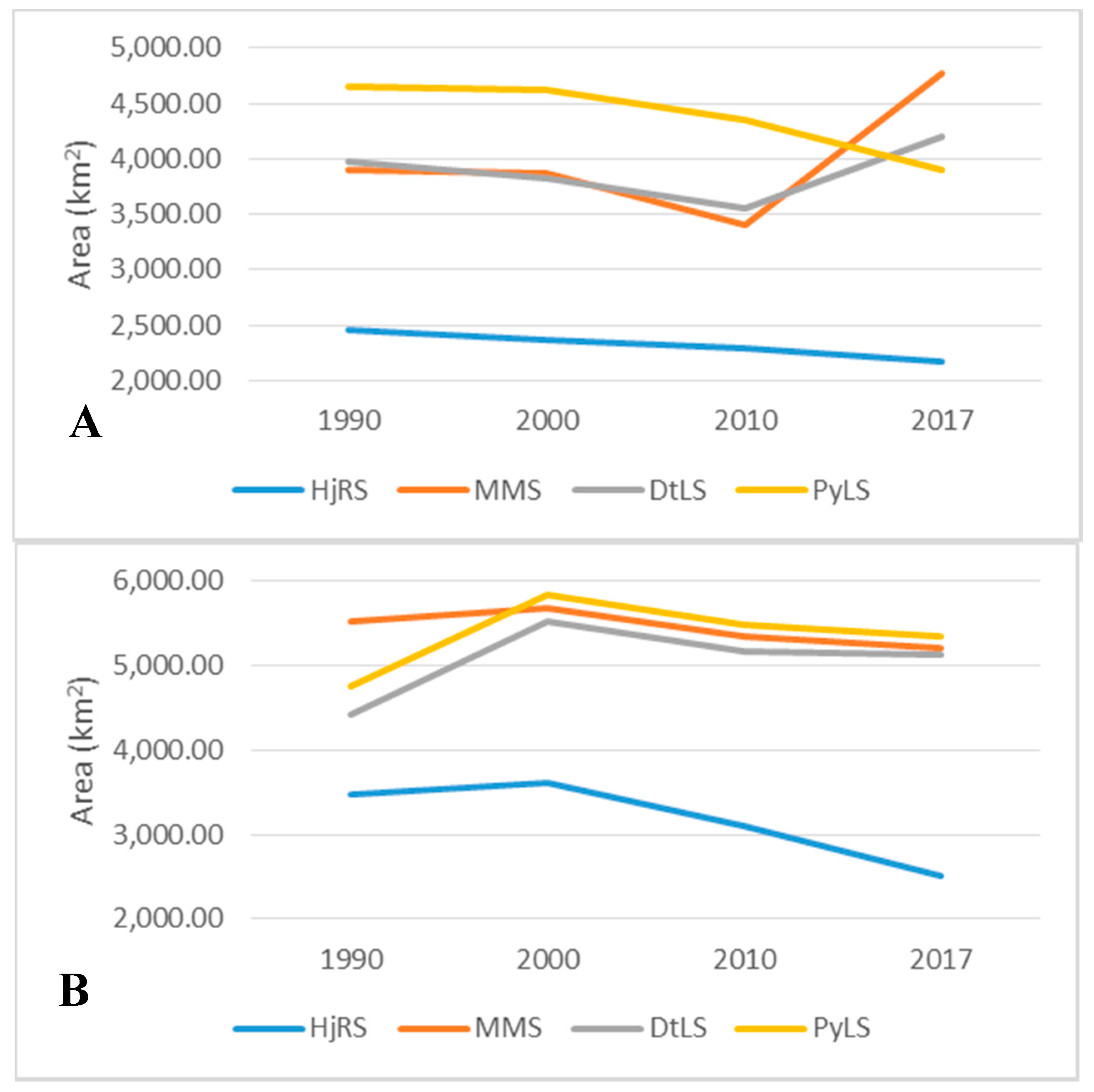
| HjRS | MMS | DtLS | PyLS | HjRS | MMS | DtLS | PyLS | |
| 1990 | 2460.83 | 3905.78 | 3977.60 | 4653.30 | 3480.74 | 5529.63 | 4416.59 | 4747.23 |
| 2000 | 2361.32 | 3864.66 | 3819.39 | 4618.39 | 3622.48 | 5683.64 | 5521.68 | 5842.19 |
| 2010 | 2293.17 | 3408.31 | 3551.97 | 4357.58 | 3092.42 | 5352.60 | 5168.93 | 5483.36 |
| 2017 | 2170.22 | 4768.98 | 4204.66 | 3906.24 | 2519.38 | 5217.12 | 5141.00 | 5357.59 |
© 2018 by the authors. Licensee MDPI, Basel, Switzerland. This article is an open access article distributed under the terms and conditions of the Creative Commons Attribution (CC BY) license (http://creativecommons.org/licenses/by/4.0/).
Share and Cite
Wang, C.; Jia, M.; Chen, N.; Wang, W. Long-Term Surface Water Dynamics Analysis Based on Landsat Imagery and the Google Earth Engine Platform: A Case Study in the Middle Yangtze River Basin. Remote Sens. 2018, 10, 1635. https://doi.org/10.3390/rs10101635
Wang C, Jia M, Chen N, Wang W. Long-Term Surface Water Dynamics Analysis Based on Landsat Imagery and the Google Earth Engine Platform: A Case Study in the Middle Yangtze River Basin. Remote Sensing. 2018; 10(10):1635. https://doi.org/10.3390/rs10101635
Chicago/Turabian StyleWang, Chao, Mingming Jia, Nengcheng Chen, and Wei Wang. 2018. "Long-Term Surface Water Dynamics Analysis Based on Landsat Imagery and the Google Earth Engine Platform: A Case Study in the Middle Yangtze River Basin" Remote Sensing 10, no. 10: 1635. https://doi.org/10.3390/rs10101635
APA StyleWang, C., Jia, M., Chen, N., & Wang, W. (2018). Long-Term Surface Water Dynamics Analysis Based on Landsat Imagery and the Google Earth Engine Platform: A Case Study in the Middle Yangtze River Basin. Remote Sensing, 10(10), 1635. https://doi.org/10.3390/rs10101635