Permafrost Soil Moisture Monitoring Using Multi-Temporal TerraSAR-X Data in Beiluhe of Northern Tibet, China
by
 , , and
Chao Wang
1,2,*, 
Zhengjia Zhang
1,2,3,
Simonetta Paloscia
4,
Hong Zhang
1,*,
Fan Wu
1 and
Qingbai Wu
5 1
Key Laboratory of Digital Earth Science, Institute of Remote Sensing and Digital Earth, Chinese Academy of Sciences, Beijing 100094, China
2
University of Chinese Academy of Sciences, Beijing 100049, China
3
Facaulty of Information Engineering, China University of Geosciences, Wuhan 430074, China
4
Institute of Applied Physics, National Research Council, CNR-IFAC, 50019 Firenze, Italy
5
Northwest Institute of Eco-Environment and Resources, Chinese Academy of Sciences, Lanzhou 730000, China
*
Authors to whom correspondence should be addressed.
Remote Sens. 2018, 10(10), 1577; https://doi.org/10.3390/rs10101577
Submission received: 29 July 2018
/
Revised: 30 August 2018
/
Accepted: 12 September 2018
/
Published: 1 October 2018
(This article belongs to the Special Issue SAR in Big Data Era)
Abstract
:Global change has significant impact on permafrost region in the Tibet Plateau. Soil moisture (SM) of permafrost is one of the most important factors influencing the energy flux, ecosystem, and hydrologic process. The objectives of this paper are to retrieve the permafrost SM using time-series SAR images, without the need of auxiliary survey data, and reveal its variation patterns. After analyzing the characteristics of time-series radar backscattering coefficients of different landcover types, a two-component SM retrieval model is proposed. For the alpine meadow area, a linear retrieving model is proposed using the TerraSAR-X time-series images based on the assumption that the lowest backscattering coefficient is measured when the soil moisture is at its wilting point and the highest backscattering coefficient represents the water-saturated soil state. For the alpine desert area, the surface roughness contribution is eliminated using the dual SAR images acquired in the winter season with different incidence angles when retrieving soil moisture from the radar signal. Before the model implementation, landcover types are classified based on their backscattering features. 22 TerraSAR-X images are used to derive the soil moisture in Beiluhe, Northern Tibet with different incidence angles. The results obtained from the proposed method have been validated using in-situ soil moisture measurements, thus obtaining RMSE and Bias of 0.062 cm3/cm3 and 4.7%, respectively. The retrieved time-series SM maps of the study area point out the spatial and temporal SM variation patterns of various landcover types.
1. Introduction
As the highest plateau in the world, the Qinghai Tibetan Plateau (QTP) affects its surrounding environment and climate directly through atmosphere and hydrological processes [1]. The permafrost state and dynamics in QTP are sensitive indicators of global change. With the increasing trend of the global warming, more efforts in monitoring this fragile ecosystem have been carried out. Soil moisture (SM) in the permafrost region is one of the key parameters influencing the energy flux between the cryosphere and the atmosphere, the ecosystem in the cold region, etc. [2,3]. Therefore, it is important to accurately monitor the soil water-content and analyse the spatial distribution and temporal variation features.
A conventional method of monitoring SM is based on the gathering of in-situ field measurements, which can obtain soil water-content accurately on a regional scale. However, this method is time consuming and cannot provide SM map with high spatial and temporal sampling density. In recent years, remote-sensing techniques have been explored for their potential to retrieve SM. Due to the influence of the cloud and dependence on lighting, optical remote-sensing has severe limitations on SM monitoring. Active and passive microwave sensors due to the high sensitivity to water content and independence of presence of clouds and solar light have been already used for SM estimation for several decades [4,5]. Many research works have been done using synthetic aperture radar (SAR) for SM monitoring due to its high resolutions and wide coverage [6,7]. Currently, a variety of SAR sensors, such as ERS, Radarsat, PALSAR/ALOS, TerraSAR-X, Cosmo-SkyMed, and Sentinel-1, can provide images with high resolution (better than 30 m) for Earth observation and, in particular, for SM monitoring [8,9,10,11,12,13].
It is well known that the radar backscattering coefficient () from the soil surface is a function of soil surface features, which includes soil dielectric permittivity and surface roughness, as well as radar sensor configurations such as wavelength, polarization, and incidence angle [14,15]. The soil water-content is one of the factors determining the soil dielectric permittivity [16]. However, surface roughness also affects the soil dielectric permittivity, making it difficult separate the effects of these two parameters in backscattering coefficients.
SM retrieval methodologies from can be subdivided into two categories: the theoretical model and empirical/semi-empirical methods [17,18,19,20,21,22]. The Integral Equation Model (IEM) and Advanced IEM (AIEM) are widely used theoretical scattering models to retrieve the soil water-content from , covering a wide roughness validity range from very rough, as described by the geometric-optical model (GOM), to smooth surfaces, as described by the small perturbation model (SPM) [17,18,19]. However, those theoretical models are complex and can be applied with difficulty to direct SM estimations.
Another category is to use the empirical and semi-empirical models, which are built by regression of backscattering coefficients from real measurements or simulation and in situ moisture measurements in terms of different polarizations and ranges of incidence angle [20,21,22]. The most popular semi-empirical model is based on linear regressions, which characterize the relation between and SM. Linear regressions have been validated in many agricultural areas using SAR images [7,13,15]. However, those relations are site-dependent, being generally valid in a specific test site, and can therefore be barely exported and applied to other study sites, which limits their applications. Over time, more sophisticated semi-empirical models have been proposed, such as the Oh model and Dubois models [21,23,24]. The Oh model links the ratios and to both volumetric SM and surface roughness, and it is able to separate the SM effect [23,24]. This model has been validated with different band (L, C, and X) SAR images. The Dubois model described surface conditions (soil water-content and surface roughness) and sensor configurations (wavelength, polarization, and incidence angle) by using in HH and VV polarizations [21]. Many studies show that the surface roughness can be estimated more accurately using multi-angular SAR images [13,25,26,27].
Recently, with the launch of several SAR satellites and the rapid development of SAR technology and theory, various methods have been explored using SAR data in multi-modes, such as multi-frequency, multi-polarization, multi-temporal, and interferometric modes [11,28,29,30,31,32]. Meanwhile, SM retrieval from SAR images in permafrost regions is also in progress [33,34,35,36,37]. Soil roughness is one of the most significant parameters affecting SM retrieval from , especially at high frequencies, such as X band. Previous studies demonstrated that for bare agricultural plots with smooth surfaces, the effect of the soil roughness on the TerraSAR-X signal is low, and the radar signal is mainly dependent on moisture content [7,38]. However, in the Tibet plateau area, the surface is not flat and the surface roughness is not homogeneous. The effect of the surface roughness on cannot, therefore, be neglected. There are two main methods for removing the soil roughness effect from the radar signal. The first one is to use physical models, such as GOM and SPM, to simulate the effect of soil roughness. However, some real terrain situations in QTP may not meet the conditions of these models. The other one is to combine data from the physical model with real SAR data to estimate the soil roughness component. Van der Velde et al. [34,36] used three SAR images with different incidence angles and data from IEM to retrieve the soil roughness parameters in the QTP Naqu area.
The objective of this paper is to retrieve SM using multi-temporal TerraSAR-X Staring Spotlight (ST) Mode data in Beiluhe on the Northern Tibet Plateau without the need to measure ancillary data. The time-series of different landcover types has been analyzed. Indeed, a linear model has been used through the combination of the minimum and maximum of the time series SAR images. Moreover, the dual images acquired in winter with different incidence angles are used to eliminate the soil roughness contribution when retrieving soil moisture from radar signal. 22 TerraSAR-X images acquired from June 2014 to August 2016 with different incidence angles have been used for SM monitoring. The retrieved results were validated with the in-situ measured SM on 29 July and 9 August 2016. This method should enable us to retrieve the SM in other areas without the need of auxiliary survey data.
2. Test Site and Datasets
2.1. Test Site
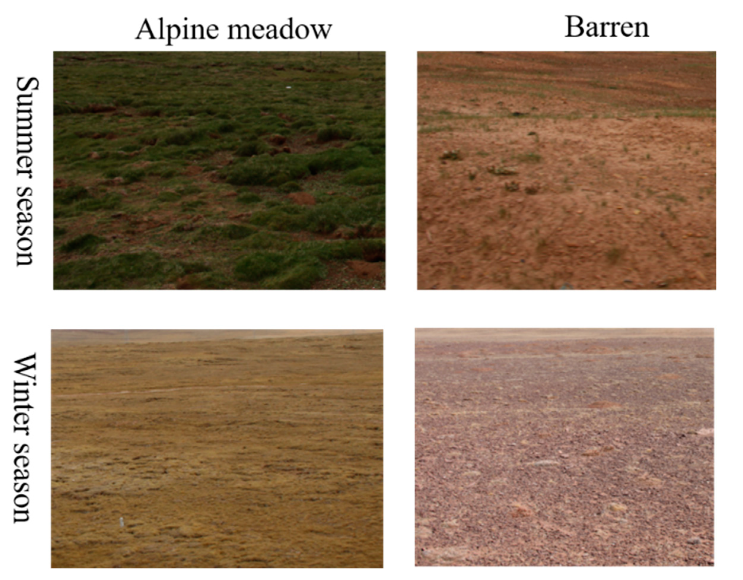
The Beiluhe permafrost region has been selected as the study site, and it is located in the southwest part of the Qinghai Province, western China (Figure 1). In Beiluhe area, elevation of the test site ranges from 4400 m to 4900 m, and the mean annul ground temperature is lower than −0.5 °C. It is low-temperature permafrost region with continuous perennial permafrost and ice-rich active layers. The ground surface is mostly covered by sandy-clay soil with gravels. The landcover types are mainly alpine meadow and alpine desert (see Figure 2) [39]. In Figure 2, it can be seen that from summer to winter season, the surfaces of mountainous slopes and gross desert show small variations, while those of alpine meadow experienced much more variations in surface characteristics. Through field investigation, it is found that most of the study area surfaces are covered with scarce vegetation, which is suitable for SM monitoring. For the alpine barren area, about 70% of the surface is covered with 10 cm gravel and 10~15% of the surface is grass. The soil component is about 15%.
The region is characterized by cold and arid climate conditions with variable annual precipitation between 50 and 400 mm, concentrated in summer season (from May to October). Rainfall and soil moisture (at 10 cm soil depth) data measured at Beiluhe weather station are shown in Figure 3, confirming the relationship between soil moisture and precipitation.
2.2. Ground Measurements
Four field campaigns were performed to collect the ground truth simultaneously to TerraSAR-X passes over the test site. One was on 8–13 March 2016, in winter. The others were on 12 August 2015, and 29 July and 9 August 2016, in summer. The Time Domain Reflectometer (TDR) probes were used to measure the volumetric SM. Soil samples were also taken to get the gravimetric SM measurements for calibrating TDR probes. The locations of the measurement samples are shown in Figure 1 (yellow pins). Those measurement samples were distributed in the study area, covering the landcover types shown in Figure 2. For each training plot, three gravimetric samples were collected at 5 cm-depth to measure the gravimetric SM. The gravimetric measurements were converted to volumetric SM based on bulk density and were used to calibrate the TDR measurements. An average of three soil bulk-density measurements was performed for each test location. The soil bulk density ranges from 1.01 to 1.59. The comparison between the gravimetrically determined SM and the TDR measured volumetric SM results in a well-defined linear relationship with Root Mean Squared Error (RMSE) of 0.039 cm3/cm3 (Figure 4), which shows that the measured SM are convincing. During the TerraSAR-X acquisition on 12 August 2015, it was raining in Beiluhe test site, and the water contents of most samples were high or even saturated. On 8 March 2016, the surface was at its wilting point, with water content around 0.03 cm3/cm3. On 28 July 2016 and 9 August 2016, the soil water-content ranged from 0.01 to 0.3 cm3/cm3.
Surface roughness parameters were measured using a 1 m-long pin profilometer with 1 cm sampling interval (See Figure 5). Eight roughness profiles were sampled for each test field in different directions. Based on those measurements, the soil roughness parameters, such as the root mean square surface height (Hrms) and the correlation length (Lc), were obtained. The Hrms values range from 0.5 cm to 1.6 cm, and the correlation length (Lc) varies from 4 to 19 cm. The soil roughness profiles were acquired only once, assuming that the surface roughness did not change during the whole observation period. The error in the soil roughness measurements is influenced mainly by the roughness profile length and sampling interval of the profiles.
2.3. SAR Datasets
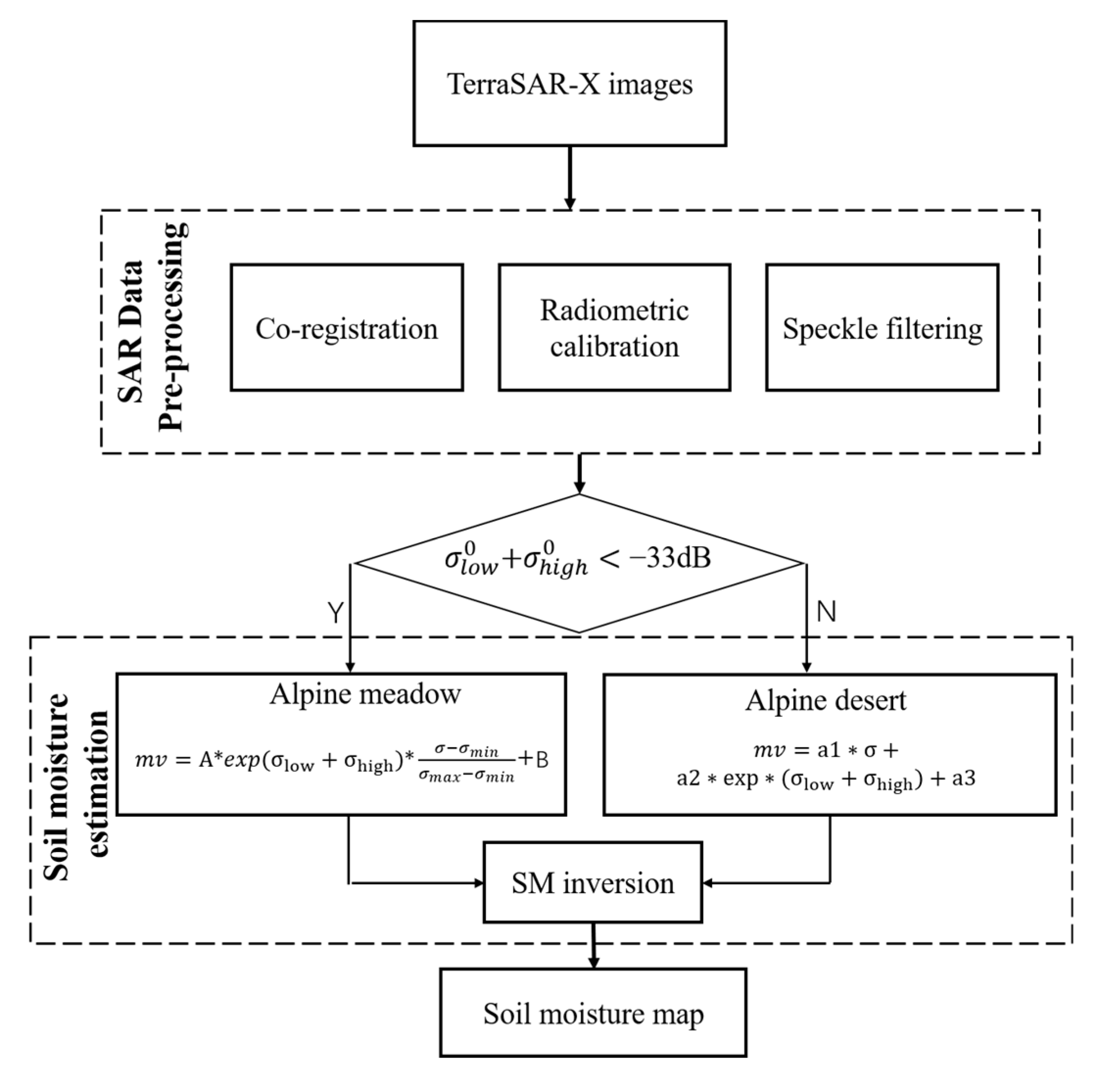
22 scenes of TerraSAR-X Staring SpotLight (ST) mode data with ‘HH’ polarization and wave length of 3.2 cm are acquired and used in this study (see Table 1). The amplitude of the SAR image is shown in Figure 1, with the area of 4 × 8 km2. The acquisition dates spanned from the June 2014 to August 2016, experiencing annual changes from the thawing season to the freezing season. The pixel spacings of the complex image in range and azimuth direction were 0.454 m and 0.167 m, respectively. All radar images were acquired in ascending orbits in right-looking direction, and at the same polarization. Two incidence angle modes were used (25.429 and 42.299).
The radar incidence angle has been taken into account in this calibration process. High-precision DEM was generated for radiometric terrain correction. In order to reduce the speckle noise, the refined Lee filter with the window size 7 × 7 was used [40]. After that, all the SAR images were co-registrated.
3. Soil Moisture Retrieval
3.1. Time-Series Radar Backscattering Coefficients
First of all, it is necessary to analyze the time-series radar backscattering coefficients of different landcovers. Figure 6 shows the variation of radar backscattering coefficients of two land cover types: alpine meadow and alpine desert areas. Four sites have been selected randomly for each type of surface.
It can be noted that the annual variations of alpine meadow and alpine desert show different trends. in alpine meadow areas shows seasonal variations with values of −20 dB in winter and −10 dB in summer, while of alpine desert areas does not show seasonal variations, with an average value from −10 dB to −15 dB. Moreover, the minimum in alpine desert area is higher than in alpine meadow area, due to the higher values of surface roughness in this region, as it can be observed from previous study and field investigations [39]. In alpine desert area, does not change greatly with the increase or decrease of SM, thus demonstrating it is mainly a function of surface roughness.
3.2. Separation of Different Landcover Types
Before retrieving the SM, it is necessary to separate landcover types in our study area. Through the previous analysis, acquired at different incidence angles in winter can be used to separate alpine meadow from desert areas. The points of different landcover types are selected randomly on the SAR images. For each point, a 7 × 7 window was used to calculate the mean value of the point. 50 alpine meadow points and 60 alpine steppe points are selected. Figure 7 shows the scatter diagram between the terms and in different land cover types. and are maximum and minimum in the time domain at a given position. and are acquired in the winter season with low and high incidence angles (25.4° and 42.2°), respectively. Those points of each landcover type in Figure 8 are randomly selected in the SAR images. In the alpine meadow area, the difference between the and values ranges from 8 to 20 dB, while the difference between and ranges from 5 to 13 dB in alpine desert area. The alpine meadow cannot, therefore, be separated using the difference only. When the information from different incidence angles is introduced, alpine meadow area can be easily separated from alpine steppe and barren area. The value of () of most alpine meadow areas is less than −33 dB. Thus, the value () could be used to separate alpine meadow and desert area.
3.3. Estimation of Soil Moisture
As it has been analyzed in Section 3.1, the time-series in alpine meadow area and alpine desert area show different patterns. Thus, two SM retrieving models are proposed: In the alpine meadow area, shows greater sensitivity to SM with respect to in alpine desert, and a linear model has been used through scaling observations between maximum and minimum. In the alpine desert area, the radar signal is mainly a function of surface roughness based on the analysis of time-series . The dual images acquired in winter with different incidence angles are therefore used to eliminate the soil roughness contribution from the radar signal.
(A) SM retrieval model for alpine meadow
From the analysis of the time-series of TerraSAR-X data in Section 3.1, given any position in the alpine meadow area, it is assumed that the lowest were measured when the SM was at its wilting point, whereas the highest values correspond to the water-saturated soil state. Backscatter coefficient is a function of both time and local incidence angle. Then, the relationship between radar signal and SM is defined as follows:
in which and are maximum and minimum backscattering coefficients in the time domain at a given position. In this model, the first term controls the maximum and minimum values of SM. Parameter A is the soil moisture change rate. In order to control the soil moisture change varies, two values, taken at different incidence angles (25.4° and 42.2°), have been used. Then, Equation (1) can be written as follows:
(B) SM retrieval model for alpine desert
From the analysis carried out in Section 3.1, it is found that the time-series in alpine desert area do not show seasonal significant variations. The SM in alpine desert could therefore not be accurately retrieved using Equation (2). In the alpine desert area, surface roughness plays the main role in the radar signal, and therefore the effect of surface roughness should be removed in order to estimate SM. Several studies have found that the use of SAR images with different incidence angles could be useful for monitoring the surface roughness effects [13,26,27]. When using two or more SAR images with different incidence angles, it is assumed that the soil roughness does not change and that the variations in are caused by the changes of soil water-content. In this study, the dual images acquired in winter with different incidence angles are used to eliminate the soil roughness effect in the alpine desert area.
The relationship between backscatter and surface roughness could be written as an exponential or a logarithmic form [23,38]. Considering the sensitivities of radar signal to SMv and roughness, the empirical model is given by
in which SMv is volumetric soil moisture, in cm3/cm3; and and are the backscattering coefficients collected at low and high incidence angles (25.4° and 42.2°), respectively, in the winter season. a1, a2, and a3 are the unknown experimental parameters.
Based on the field investigations, the maximum and minimum of the SM are 0.4 and 0.03 in cm3/cm3 at the saturated and dried conditions in the whole study area. Using the maximum and minimum values of the time-series , the experimental tuning coefficients in Equations (2) and (3) can be solved at each point. After getting these parameters, SM can be retrieved through the proposed model for a given new TerraSAR-X image. It should be pointed out that no auxiliary survey data are necessary for retrieving SM in our study.
It should be noted that the effects of vegetation on the TerraSAR-X backscattering coefficient are neglected for the following two reasons: (1) Previous studies indicated that the contribution of vegetation to the variability is limited [34,36] in Tibet permafrost; (2) In our area, the height of alpine meadow is about 5 cm, assuming that radar signal can penetrate alpine meadow. In Section 5, the effect of the vegetation on the SM will be discussed.
The flow chart of the proposed method is shown in Figure 8. Considering the characteristic of time-series backscattering coefficients of different landcover types, two SM retrieving models have been proposed, respectively. For the alpine meadow area, a linear retrieving model is proposed combining the minimum and maximum of the SAR images time series. For the alpine desert area, the dual images acquired in winter with different incidence angles are used to eliminate the soil roughness contribution.
4. Experimental Results and Validation
After the pre-processing phase, which mainly consists of radiometric calibration, terrain correction, speckle filtering, and co-registration, SM could be retrieved using the models proposed in Section 3. The inversion performance is evaluated through three of the most-used statistic parameters, i.e., the determination coefficient (R2), the Root Mean Square Error (RMSE), and the mean bias (Bias).
4.1. Time-Series Approach Results
First of all, the images acquired in the winter with the incidence angles of 25.4° and 42.2° are used to identify the alpine meadow and desert areas. Then, of time-series TerraSAR-X images, at low and high incidence angles in winter season (13 December 2014 and 9 January 2015), and maximum and minimum SM values of 0.03 and 0.4 for each pixel are used as inputs for solving Equations (2) and (3). After getting the constant coefficients, the SM map of the area can be generated for a given TerraSAR-X image and, consequently, the time-series of SM of the study area.
Figure 9 illustrates the SM on 12 August 2015 and 29 July 2016. The SM values of the alpine meadow, in the lower left, as well as fluvial low lands, are high and even saturated on 12 August 2015. This is due to the rainfall that occurred on 12 August 2015. On 29 July 2016, the SM of the alpine meadow is high with a maximum value over 0.35 cm3/cm3, whereas in the alpine steppe and barren areas, the SM values are low, which is consistent with field investigations.
The validation of the SM retrieval method was carried out by comparing in-situ measurements of SM and SM estimated from TerraSAR-X using the inversion model (Equation (2) and (3)). 34 measurement samples collected in 29 July 2016 and 9 August 2016 have been used to validate the retrieval results. Figure 10 shows the comparison between the measured and the time-series approach estimated SM. The R2, RMSE, and bias are 0.66, 0.062 cm3/cm3, and 0.047, respectively. The result shows that proposed models can monitor the temporal and spatial variations of SM in QTP.
In the scatter plots, the slope of correlation line is 0.689, with the points a little dispersed, showing some over estimations. A couple of points, which correspond to plots located in alpine meadow areas, are underestimated in the high SM range. This fact could be attributed to the vertical SM gradient near the land-atmosphere interface [36], which causes the top layer to become dry, while the deeper soil remains moist. The measured SM sites are sampled at 5 cm depth, while the at X-band provides information on the topsoil only. The assumption that the maximum SM of the study area is 0.4 cm3/cm3, which may not fit the alpine desert area, may cause the overestimation.
4.2. Time-Series Soil Moisture Mapping
Figure 11 shows the temporal evolution of SM during the whole observation period using the time-series approach. These time-series SM maps could be used to monitor the temporal variation of SM during the thawing and freezing cycle. At the beginning of May, due to the thawing of the active layer, the SM of the study area begins to increase, especially in alpine meadow area, with the maximum values larger than 0.35 cm3/cm3. During the following months, in summer season, the SM is quite stable in this area, which is consistent with the dynamics of Tibetan wetland. The soil map on 12 August 2015 shows high level of SM across the whole study domain due to raining that day. Even in most of alpine steppe and barren areas, the SM is larger than 0.2 cm3/cm3. At the end of November, due to the decrease of the temperature, winter air is very dry, and the surface SM of the study area begins to decrease. It should be noted that, during the whole winter season, the SM is at the wilting point values <0.1 cm3/cm3, while the SM in alpine desert area is relatively higher than that in alpine meadow area in winter season (see Figure 11), which is not consistent with the field investigation. This discrepancy may be due to the maximum SM assumption of the study area, which overestimates the SM of alpine desert area.
Compared to the summer season in 2015, lower soil moisture values are retrieved during the summer season in 2016. The wind, the amount of rainfall, and air temperature may contribute to this SM decrease in 2016.
5. Discussions
The comparison between the SM retrieval results with the measurements indicates that the proposed method produces reasonable SM products. However, some samples show large errors. It should also consider that the effects of the vegetation are not taken into account and that the soil roughness is represented by using exp(). In this section, these effects are discussed.
5.1. The Effect of Soil Roughness
The estimate of soil surface roughness is an important task in retrieving SM. Firstly, we tried to estimate the soil roughness using AIEM model, which is similar to the method used in [39]. However, the estimated soil roughness range is small and is not representative of the surface roughness conditions of our study area [37]. From field investigations, it was found that the surface roughness shows much larger intervals, which cannot be described by physical model. It is impossible to measure Hrms and Lc at every point in the image. Thus, the ratio is used to eliminate the effect of the soil roughness from radar signal in alpine desert area.
In the time-series SM maps in Figure 11, we can see that the SM value of most the alpine desert area is about 0.15 cm3/cm3, which is higher than the field measured data. There may be two reasons for these discrepancies: (1) The surface roughness components have not been eliminated clearly and (2) In the retrieval process, it is assumed that the maximum SM value is 0.4 cm3/cm3 in the entire area. However, the SM value in alpine desert area may be lower than 0.4 cm3/cm3. This assumption may result in the overestimation of SM in alpine desert area in winter season.
5.2. The Effect of Vegetation
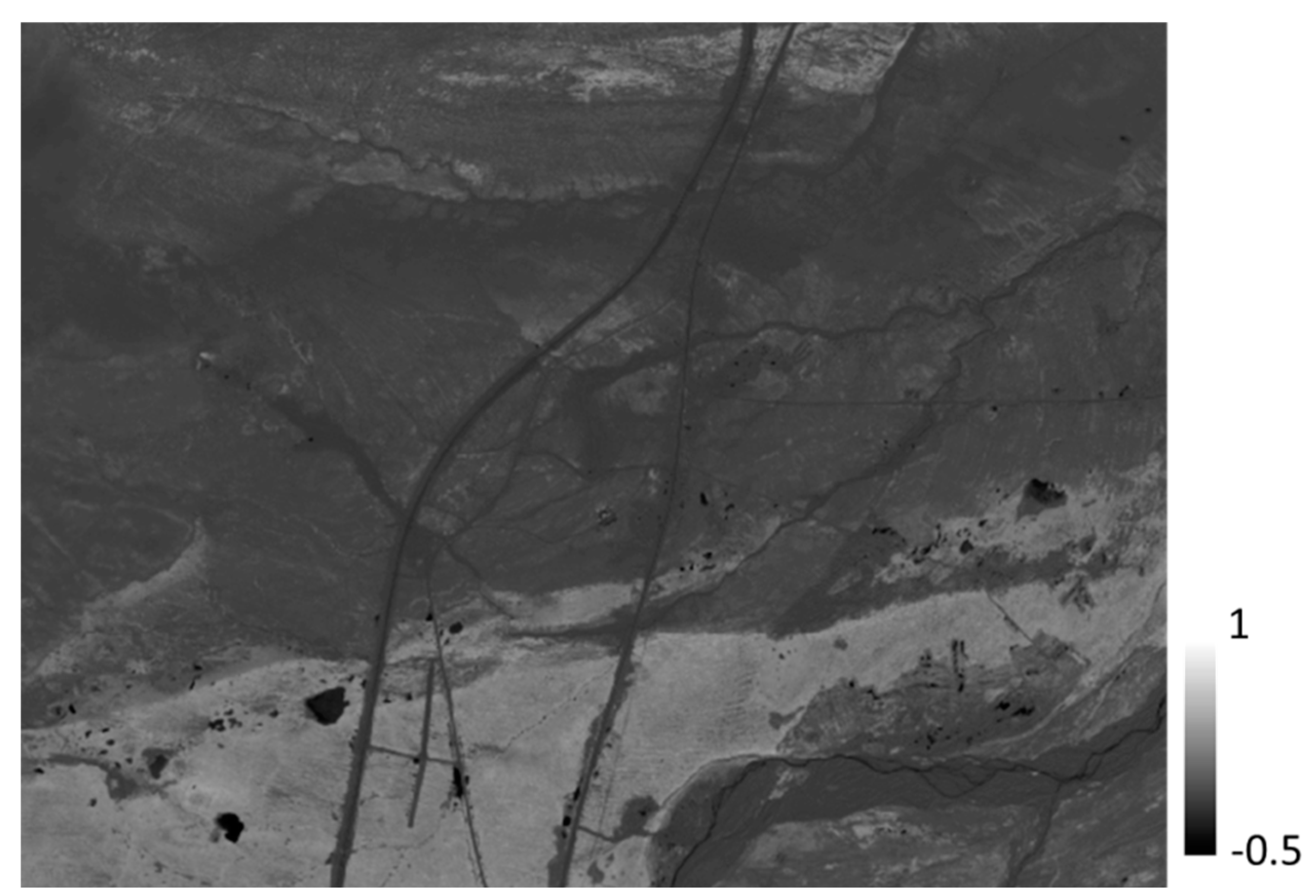
In this paper, the influence of vegetation has been ignored. Based on field investigations, most of the study area is bare soil or is covered by sparse vegetation with height of about 5 cm. From Figure 12, in which the NDVI map of the study area obtained using Gaofen-1 optical image on 18 July 2016 is represented, we can see that even in the alpine meadow area, the NDVI value is less than 0.3, and in other area the NDVI value is about 0. Van der Velde et al. found that the σo time series from both the grassland and wetland areas has only a weak correlation with the NDVI via a multivariate analysis [34].
On the other hand, it should be considered that the growth of vegetation is correlated with the SM. Higher SM will contribute to denser vegetation, though it will be small in absolute terms. The vegetation and SM share a similar effect on the radar signal. Thus, in this study site, the assumption of neglecting the effect of vegetation is reasonable, since it does not affect the accuracy of SM maps.
6. Conclusions
Permafrost SM is an important factor controlling the energy flux in the Tibet Plateau. The objectives of this study are to retrieve SM in the permafrost area using the time-series method with single polarization SAR images and to reveal its spatial and temporal variations. In this study, 22 scenes of TerraSAR-X ST mode data with different incidence angles are used to retrieve the SM in Beiluhe, Northern Tibet. Considering the characteristic of the time-series backscattering coefficients of different landcovers, a dual SM retrieving model is proposed. The main conclusions are summarized as follows:
- (1)
- It is found that the time-series of of alpine meadow areas show seasonal variations, with −20 dB in winter and −10 dB in summer, whereas the of alpine desert areas do not show seasonal variations.
- (2)
- The term derived from two images acquired in winter season with different incidence angles can be used to eliminate the soil roughness variable when retrieving SM from radar signal. Moreover, the term could be used to separate the alpine meadow and desert area.
- (3)
- In Beiluhe area, time-series SM maps are retrieved from ° of TerraSAR-X with RMSE of 0.062 cm3/cm3 in comparison with in-situ measurements. These results validate the feasibility of the proposed methodology.
- (4)
- The retrieved time-series SM maps point out the spatial and temporal variation patterns in the test site. The SM variations are correlated with thawing and freezing cycles, and with those of the alpine meadow that show more regular seasonal variations.
The major advantage of the proposed methods is that they could retrieve SM without the need for auxiliary survey data, such as field-measured SM and surface roughness. Further work will be focused on SM monitoring using the model in large-scale permafrost areas without knowing the actual values of surface roughness.
Author Contributions
Methodology, C.W., Z.Z. and S.P.; Software, Z.Z.; Validation, H.Z., F.W. and Q.W.; Writing-Original Draft Preparation, C.W., Z.Z.; Writing-Review & Editing, S.P., H.Z.; Supervision, C.W., H.Z.; Project Administration, C.W.; Funding Acquisition, C.W.
Funding
This research was funded by the National Natural Science Foundation of China (41331176), and National Key Research and Development Program of China (2016YFB0501501).
Acknowledgments
This paper is under the project of TerraSAR-X New Modes AO (ID: HYD2420) and is funded by the National Natural Science Foundation of China (NSFC) under the Grant 41331176, 41330634. All TerraSAR-X data was provided by DLR. The authors would like to thank K.S. Chen (CAS-RADI) for providing the AIEM source code; Lin Zhao (CAS-NIEER) for field support; and Bo Zhang, Jinxing Chen, Mingzhe Zhang, and Lei Liu et al. for field work.
Conflicts of Interest
The authors declare no conflict of interest.
References
- Yang, K.; Ye, B.; Zhou, D.; Wu, B.; Foken, T.; Qin, J.; Zhou, Z. Response of hydrological cycle to recent climate changes in the Tibetan Plateau. Clim. Chang. 2011, 109, 517–534. [Google Scholar] [CrossRef]
- Yang, K.; Qin, J.; Zhao, L.; Chen, Y.; Tang, W.; Han, M.; Lin, C. A multiscale soil moisture and freeze-thaw monitoring network on the third pole. Bull. Am. Meteorol. Soc. 2013, 94, 1907–1916. [Google Scholar] [CrossRef]
- Su, Z.; Wen, J.; Dente, L.; van der Velde, R.; Wang, L.; Ma, Y.; Yang, K.; Hu, Z. The Tibetan Plateau observatory of plateau scale soil moisture and soil temperature (Tibet-Obs) for quantifying uncertainties in coarse resolution satellite and model products. Hydrol. Earth Syst. Sci. 2011, 15, 2303–2316. [Google Scholar] [CrossRef] [Green Version]
- Jackson, T.J. Measuring surface soil moisture using passive microwave remote sensing. Hydrol. Process. 1993, 7, 139–152. [Google Scholar] [CrossRef]
- Paloscia, S.; Macelloni, G.; Santi, E.; Koike, T. A multifrequency algorithm for the retrieval of soil moisture on a large scale using microwave data from SMMR and SSM/I satellites. IEEE Trans. Geosci. Remote Sens. 2001, 39, 79–93. [Google Scholar] [CrossRef]
- Shi, J.C.; Wang, J.; Hsu, A.Y.; O’Neill, P.E.; Engman, E.T. Estimation of bare surface soil moisture and surface roughness parameter using L-band SAR image data. IEEE Trans. Geosci. Remote Sens. 1997, 35, 1254–1266. [Google Scholar]
- Aubert, M.; Baghdadi, N.; Zribi, M.; Ose, K.; Hajj, M.; Vaudour, E.; Sosa, E. Toward an Operational Bare Soil Moisture Mapping Using TerraSAR-X Data Acquired Over Agricultural Areas. IEEE J. Sel. Top. Appl. Earth Obs. Remote Sens. (JSTARS) 2013, 6, 900–916. [Google Scholar] [CrossRef] [Green Version]
- Zhang, X.; Zhao, J.; Sun, Q.; Wang, X.; Guo, Y.; Li, J. Soil moisture retrieval from AMSR-E data in Xinjiang (China): Models and validation. IEEE J. Sel. Top. Appl. Earth Obs. Remote Sens. (JSTARS) 2011, 4, 117–127. [Google Scholar] [CrossRef]
- Baghdadi, N.; Cerdan, O.; Zribi, M.; Auzet, V.; Darboux, F.; ElHajj, M. Operational performance of current synthetic aperture radar sensors in mapping soil surface characteristics in agricultural environments: Application to hydrological and erosion modelling. Hydrol. Process. 2008, 22, 9–20. [Google Scholar] [CrossRef]
- Le Hegarat-Mascle, S.; Zribi, M.; Alem, F.; Weisse, A.; Loumagne, C. Soil moisture estimation from ERS/SAR data: Toward an operational methodology. IEEE Trans. Geosci. Remote Sens. 2002, 40, 2647–2658. [Google Scholar] [CrossRef]
- Balenzano, A.; Mattia, F.; Satalino, G.; Davidson, M.W.J. Dense temporal series of C- and L-band SAR data for soil moisture retrieval over agricultural crops. IEEE J. Sel. Top. Appl. Earth Obs. Remote Sens. (JSTARS) 2011, 4, 439–450. [Google Scholar] [CrossRef]
- Merzouki, A.; McNairn, H.; Pacheco, A. Mapping soil moisture using RADARSAT-2 data and local autocorrelation statistics. IEEE J. Sel. Top. Appl. Earth Obs. Remote Sens. (JSTARS) 2011, 4, 128–137. [Google Scholar] [CrossRef]
- Zribi, M.; Dechambre, M. A new empirical model to retrieve soil moisture and roughness from C-band radar data. Remote Sens. Environ. 2003, 84, 42–52. [Google Scholar] [CrossRef]
- Dobson, M.C.; Ulaby, F.T.; Pierce, L.E. Land-cover classification and estimation of terrain attributes using synthetic aperture radar. Remote Sens. Environ. 1995, 51, 199–214. [Google Scholar] [CrossRef]
- Ulaby, F.T.; Kouyate, F.; Brisco, B.; Williams, T.H.L. Textural infornation in SAR images. IEEE Trans. Geosci. Remote Sens. 1986, GE-24, 235–245. [Google Scholar] [CrossRef]
- Hallikainen, M.T.; Ulaby, F.T.; Dobson, M.C.; El-rayes, M.A.; Wu, L. Microwave Dielectric Behavior of Wet Soil-Part 1: Empirical-Models and Experimental Observations. IEEE Trans. Geosci. Remote Sens. 1985, 23, 25–34. [Google Scholar] [CrossRef]
- Fung, A.K.; Li, Z.; Chen, K.S. Backscattering from a Randomly Rough Dielectric Surface. IEEE Trans. Geosci. Remote Sens. 1992, 30, 356–369. [Google Scholar] [CrossRef]
- Wu, T.D.; Chen, K.S. A Reappraisal of the Validity of the IEM Model for Backscattering from Rough Surfaces. IEEE Trans. Geosci. Remote Sens. 2004, 42, 743–753. [Google Scholar]
- Chen, K.S.; Wu, T.D.; Tsang, L.; Li, Q.; Shi, J.C.; Fung, A.K. Emission of Rough Surfaces Calculated by the Integral Equation Method with Comparison to Three-Dimensional Moment Method Simulations. IEEE Trans. Geosci. Remote Sens. 2003, 41, 90–101. [Google Scholar] [CrossRef]
- Oh, Y. Quantitative Retrieval of Soil Moisture Content and Surface Roughness from Multipolarized Radar Observations of Bare Soil Surfaces. IEEE Trans. Geosci. Remote Sens. 2004, 42, 596–601. [Google Scholar] [CrossRef]
- Dubois, P.C.; van Zyl, J.; Engman, T. Measuring soil moisture with imaging radars. IEEE Trans. Geosci. Remote Sens. 1995, 33, 915–926. [Google Scholar] [CrossRef] [Green Version]
- Rahman, M.M.; Moran, M.S.; Thoma, D.P.; Bryant, R.; Collins, C.D.H.; Jackson, T.; Orr, B.J.; Tischler, M. Mapping Surface Roughness and Soil Moisture Using Multi-Angle Radar Imagery without Ancillary Data. Remote Sens. Environ. 2008, 112, 391–402. [Google Scholar] [CrossRef]
- Oh, Y.; Sarabandi, K.; Ulaby, F.T. An empirical model and an inversion technique for radar scattering from bare soil surfaces. IEEE Trans. Geosci. Remote Sens. 1992, 30, 370–381. [Google Scholar] [CrossRef]
- Oh, Y.; Kay, Y.C. Condition for precise measurement of soil surface roughness. IEEE Trans. Geosci. Remote Sens. 1998, 36, 691–695. [Google Scholar]
- Zribi, M.; Baghdadi, N.; Holah, N.; Fafin, O.; Guérin, C. Evaluation of a rough soil surface description with ASAR-ENVISAT Radar Data. Remote Sens. Environ. 2005, 95, 67–76. [Google Scholar] [CrossRef]
- Baghdadi, N.; Holah, N.; Zribi, M. Soil Moisture Estimation Using Multi-Incidence and Multi-Polarization ASAR Data. Int. J. Remote Sens. 2006, 27, 1907–1920. [Google Scholar] [CrossRef]
- Srivastava, H.S.; Patel, P.; Manchanda, M.; Adiga, S. Use of multi-incidence angle RADARSAT-1 SAR data to incorporate the effect of surface roughness in soil moisture estimation. IEEE Trans. Geosci. Remote Sens. 2003, 41, 1638–1640. [Google Scholar] [CrossRef]
- Hajnsek, I.; Jagdhuber, T.; Schön, H.; Papathanassiou, K.P. Potential of Estimating Soil Moisture under Vegetation Cover by Means of PolSAR. IEEE Trans. Geosci. Remote Sens. 2009, 47, 442–454. [Google Scholar] [CrossRef] [Green Version]
- Paloscia, S.; Macelloni, G.; Pampaloni, P.; Santi, E. The Contribution of Multitemporal SAR Data in Assessing Hydrological Parameters. IEEE Trans. Geosci. Remote Sens. Lett. 2004, 1, 201–205. [Google Scholar] [CrossRef]
- Nolan, M.; Fatland, D.R.; Hinzman, L. DInSAR Measurements of Soil Moisture. IEEE Trans. Geosci. Remote Sens. 2003, 41, 2802–2813. [Google Scholar] [CrossRef]
- Hajnsek, I.; Prats, P. Soil Moisture Estimation in Time with D-InSAR. In Proceedings of the IGARSS 2008, Boston, MA, USA, 7–11 July 2008; pp. 546–549. [Google Scholar]
- De Zan, F.; Parizzi, A.; Prats-Iraola, P.; López-Dekker, P. A SAR Interferometric Model for Soil Moisture. IEEE Trans. Geosci. Remote Sens. 2014, 52, 418–425. [Google Scholar] [CrossRef] [Green Version]
- Sabel, D.; Bartsch, A.; Schlaffer, S.; Klein, J.-P.; Wagner, W. Soil Moisture Mapping in Permafrost Regions-An Outlook to Sentinel-1. In Proceedings of the IGARSS 2012, Munich, Germany, 22–27 July 2012; pp. 1216–1219. [Google Scholar]
- Van der Velde, R.; Su, Z. Dynamics in land-surface conditions on the Tibetan Plateau observed by Advanced Synthetic Aperture Radar (ASAR). Hydrol. Sci. J. 2009, 54, 1079–1093. [Google Scholar] [CrossRef] [Green Version]
- Tang, W.; Kelly, R. Sensitivity of Radarsat-2 Quad Polarimetric and Simulated Compact Polarimetric Parameters to Soil Moisture and Freeze/Thaw State in Southwest Ontario. In Proceedings of the IEEE IGARSS 2014, Quebec City, QC, Canada, 13–18 July 2014; pp. 3232–3235. [Google Scholar]
- Van der Velde, R.; Su, Z.; van Oevelen, P.; Wen, J.; Ma, Y.; Salama, M.S. Soil moisture mapping over the central part of the Tibetan Plateau using a series of ASAR WS images. Remote Sens. Environ. 2012, 120, 175–187. [Google Scholar] [CrossRef]
- Wang, C.; Zhang, H.; Wu, Q.; Zhang, Z.; Xie, L. Monitoring permafrost soil moisture with multi-temporal TerraSAR-X data in northern Tibet. In Proceedings of the IEEE IGARSS 2016, Beijing, China, 10–15 July 2016; pp. 3039–3042. [Google Scholar]
- Aubert, M.; Baghdadi, N.; Zribi, M.; Douaoui, A.; Loumagne, C.; Baup, F.; El Hajje, M.; Garrigues, S. Analysis of TerraSAR-X data sensitivity to bare soil moisture, roughness, composition and soil crust. Remote Sens. Environ. 2011, 115, 1801–1810. [Google Scholar] [CrossRef] [Green Version]
- Wu, Q.; Hou, Y.; Yun, H.; Liu, Y. Changes in active-layer thickness and near-surface permafrost between 2002 and 2012 in alpine ecosystems, Qinghai–Xizang (Tibet) Plateau, China. Glob. Planet. Chang. 2015, 124, 149–155. [Google Scholar] [CrossRef]
- Lee, J.S.; Grunes, M.; Pottier, E.; Ferro-Famil, L. Segmentationof polarimetric SAR images. In Proceedings of the IGARSS, Sydney, Australia, 9–13 July 2001; Volume 1, pp. 414–416. [Google Scholar]
Figure 1.
Map of the test site and the TerraSAR-X ST mode data coverage. Yellow pins are the measurement locations. Background is the Google map.
Figure 1.
Map of the test site and the TerraSAR-X ST mode data coverage. Yellow pins are the measurement locations. Background is the Google map.

Figure 2.
Field photos of typical land covers of the study site in summer and winter seasons.

Figure 3.
Soil moisture at a 10 cm soil depth and rainfall measured at Beiluhe weather station.

Figure 4.
Comparison of TDR-measured SM against gravimetrically determined volumetric SM.
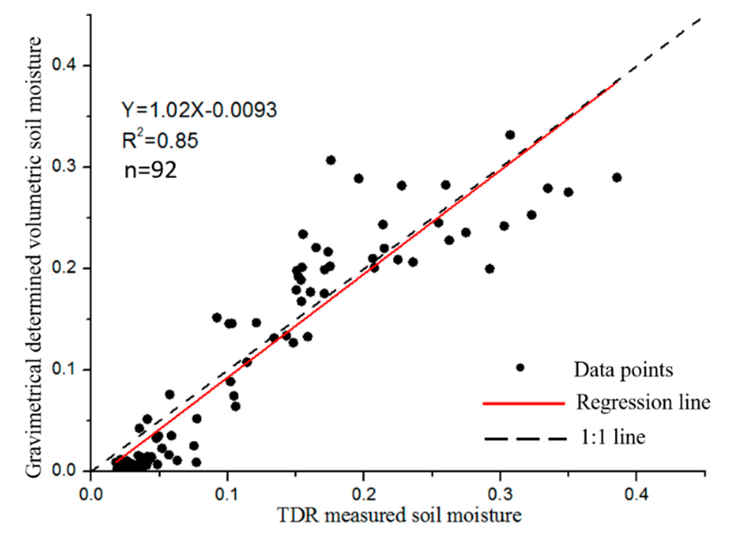
Figure 5.
Example of a roughness profile with a 1 m long needle profilometer and a 1 cm interval between needles.
Figure 5.
Example of a roughness profile with a 1 m long needle profilometer and a 1 cm interval between needles.
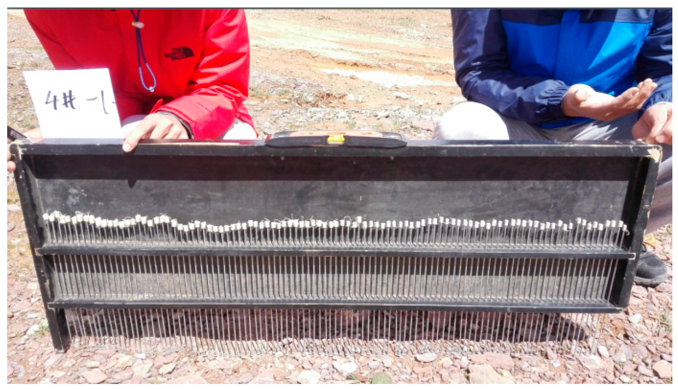
Figure 6.
variations for two different land cover types: (a) alpine meadow area and (b) alpine desert area.
Figure 6.
variations for two different land cover types: (a) alpine meadow area and (b) alpine desert area.
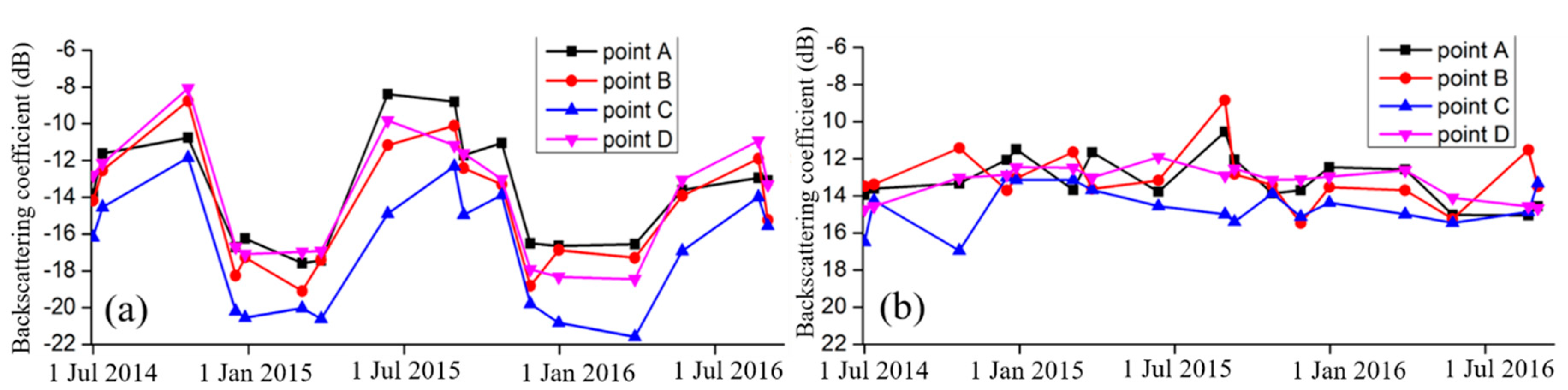
Figure 7.
Scatter plot between the () and ().
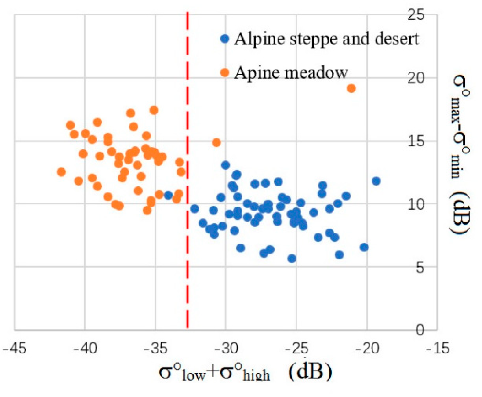
Figure 8.
Flowchart for the proposed SM estimation models.

Figure 9.
SM, in cm3/cm3 retrieved using the time series approach on 12 August 2015 and 29 July 2016. Black areas are masks of open water, railway, and highway.
Figure 9.
SM, in cm3/cm3 retrieved using the time series approach on 12 August 2015 and 29 July 2016. Black areas are masks of open water, railway, and highway.
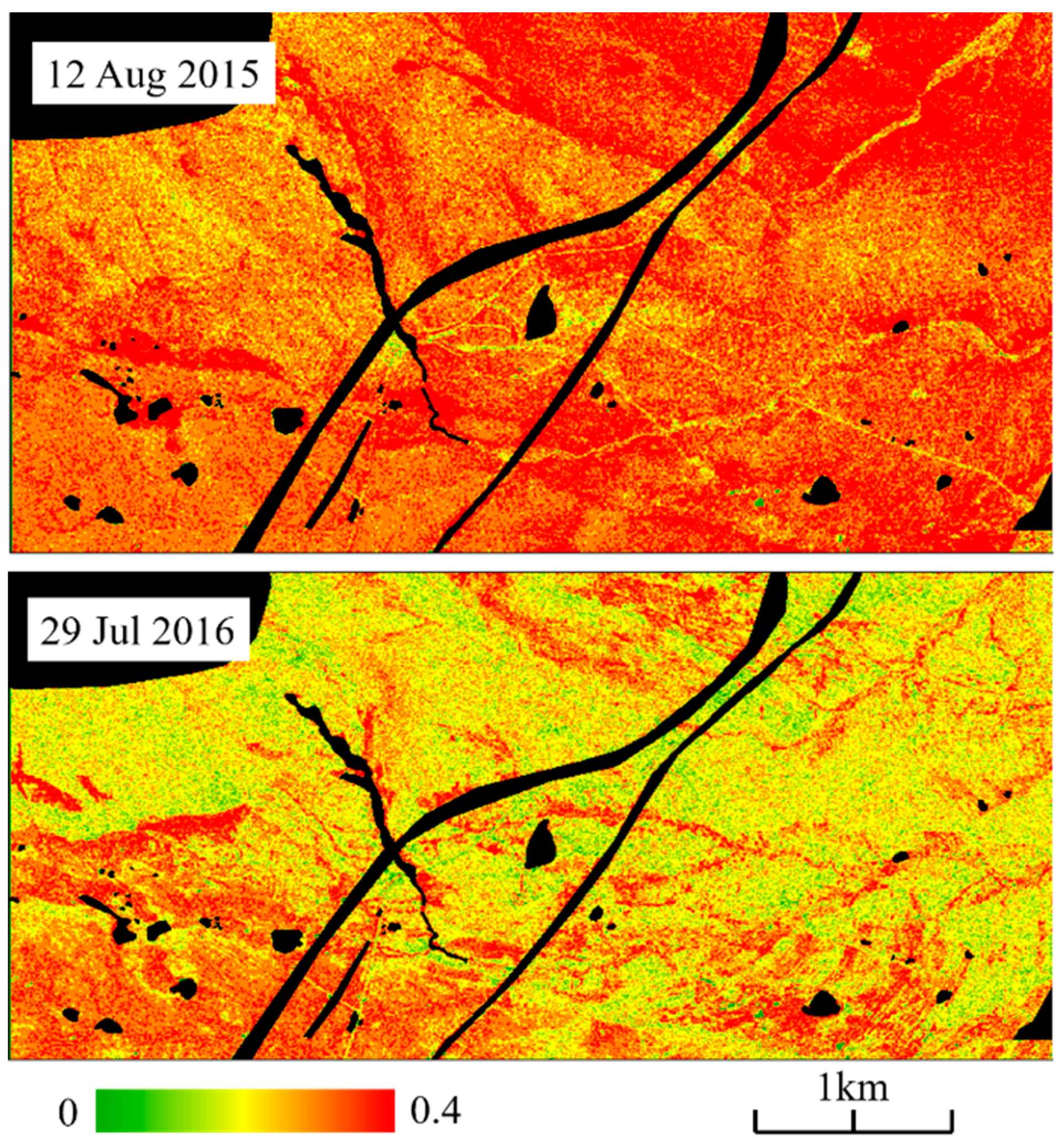
Figure 10.
Comparison between SM-retrieved soil moisture using the time series approach and in- situ-measured SM.
Figure 10.
Comparison between SM-retrieved soil moisture using the time series approach and in- situ-measured SM.
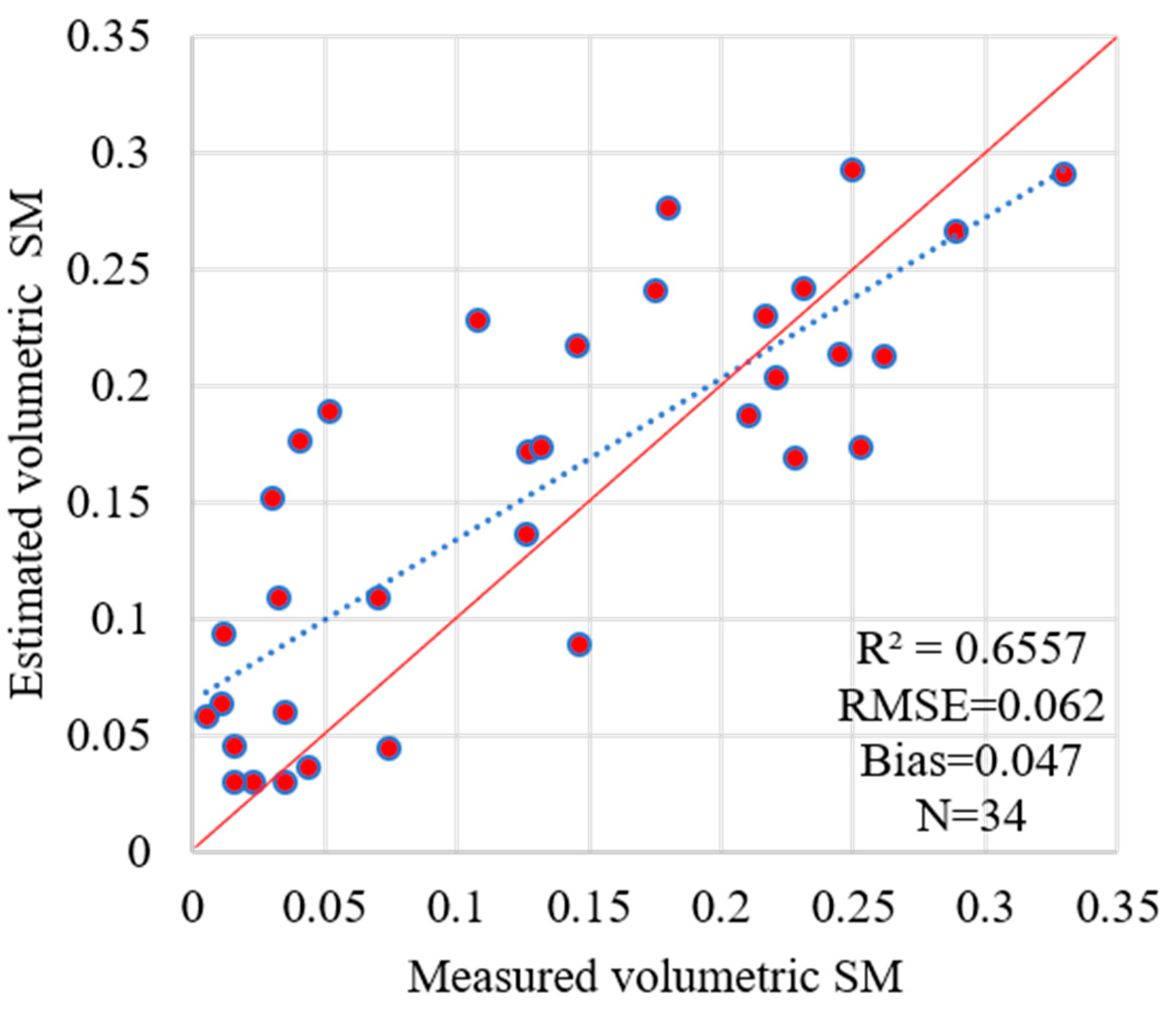
Figure 11.
Series of soil moisture maps retrieved from TerraSAR-X using the time-series approach during the whole observation period. Black areas are masks of open water, railway, and highway.
Figure 11.
Series of soil moisture maps retrieved from TerraSAR-X using the time-series approach during the whole observation period. Black areas are masks of open water, railway, and highway.

Figure 12.
NDVI map of the study area using GF-1 on 18 July 2016.

Table 1.
Parameters of the TerraSAR-X images.
| No. | Acquisition Date (dd/mm/yy) | Incidence Angle (°) | Thawing (T)/Freezing (F) Season | No. | Acquisition Date (dd/mm/yy) | Incidence Angle (°) | Thawing (T)/Freezing (F) Season |
|---|---|---|---|---|---|---|---|
| 1 | 20/06/2014 | 25.429 | T | 12 | 06/10/2015 | 25.429 | T |
| 2 | 01/07/2014 | 25.429 | T | 13 | 01/11/2015 | 25.429 | F |
| 3 | 08/10/2014 | 25.429 | T | 14 | 11/12/2015 | 25.429 | F |
| 4 | 02/12/2014 | 25.429 | F | 15 | 07/01/2016 | 42.299 | F |
| 5 | 13/12/2014 | 25.429 | F | 16 | 24/01/2016 | 25.429 | F |
| 6 | 09/01/2015 | 42.299 | F | 17 | 08/03/2016 | 25.429 | F |
| 7 | 17/02/2015 | 25.429 | F | 18 | 13/03/2016 | 42.299 | F |
| 8 | 11/03/2015 | 25.429 | F | 19 | 02/05/2016 | 25.429 | T |
| 9 | 27/05/2015 | 25.429 | T | 20 | 29/07/2016 | 25.429 | T |
| 10 | 12/08/2015 | 25.429 | T | 21 | 03/08/2016 | 42.299 | T |
| 11 | 23/08/2015 | 25.429 | T | 22 | 09/08/2016 | 25.429 | T |
© 2018 by the authors. Licensee MDPI, Basel, Switzerland. This article is an open access article distributed under the terms and conditions of the Creative Commons Attribution (CC BY) license (http://creativecommons.org/licenses/by/4.0/).
Share and Cite
MDPI and ACS Style
Wang, C.; Zhang, Z.; Paloscia, S.; Zhang, H.; Wu, F.; Wu, Q. Permafrost Soil Moisture Monitoring Using Multi-Temporal TerraSAR-X Data in Beiluhe of Northern Tibet, China. Remote Sens. 2018, 10, 1577. https://doi.org/10.3390/rs10101577
AMA Style
Wang C, Zhang Z, Paloscia S, Zhang H, Wu F, Wu Q. Permafrost Soil Moisture Monitoring Using Multi-Temporal TerraSAR-X Data in Beiluhe of Northern Tibet, China. Remote Sensing. 2018; 10(10):1577. https://doi.org/10.3390/rs10101577
Chicago/Turabian StyleWang, Chao, Zhengjia Zhang, Simonetta Paloscia, Hong Zhang, Fan Wu, and Qingbai Wu. 2018. "Permafrost Soil Moisture Monitoring Using Multi-Temporal TerraSAR-X Data in Beiluhe of Northern Tibet, China" Remote Sensing 10, no. 10: 1577. https://doi.org/10.3390/rs10101577
Note that from the first issue of 2016, this journal uses article numbers instead of page numbers. See further details here.