A Comparison of Regression Techniques for Estimation of Above-Ground Winter Wheat Biomass Using Near-Surface Spectroscopy


Abstract
:
1. Introduction
- (1)
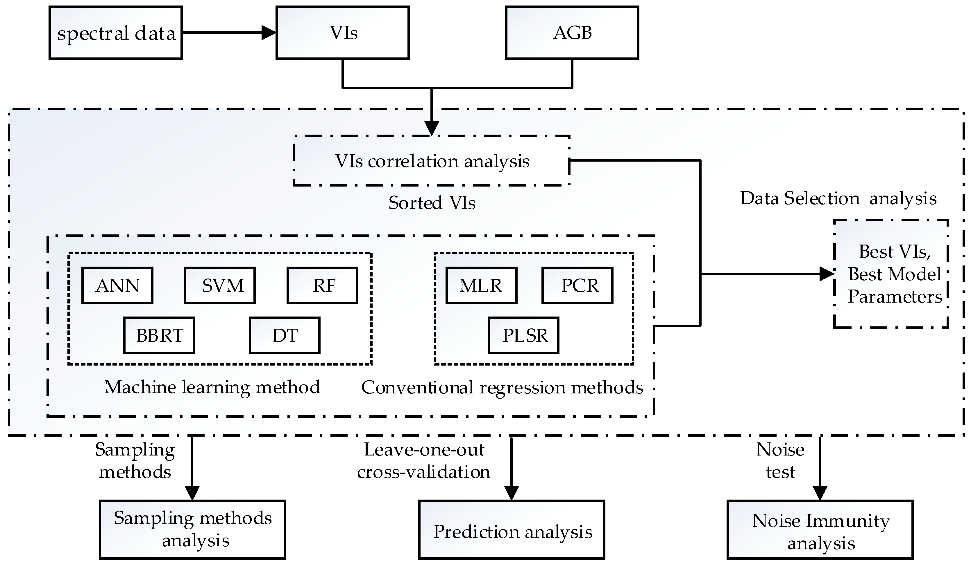
- VIs were used to train regression models, which were validated to select best VI input (Section 4.1).
- (2)
- The noise immunities of these techniques were compared by simulating remote-sensing errors by adding white Gaussian noise (Section 4.2).
- (3)
- The stability of these techniques was examined by using samples of varying sizes and different sampling methods for modeling and validation (Section 4.3).
- (4)
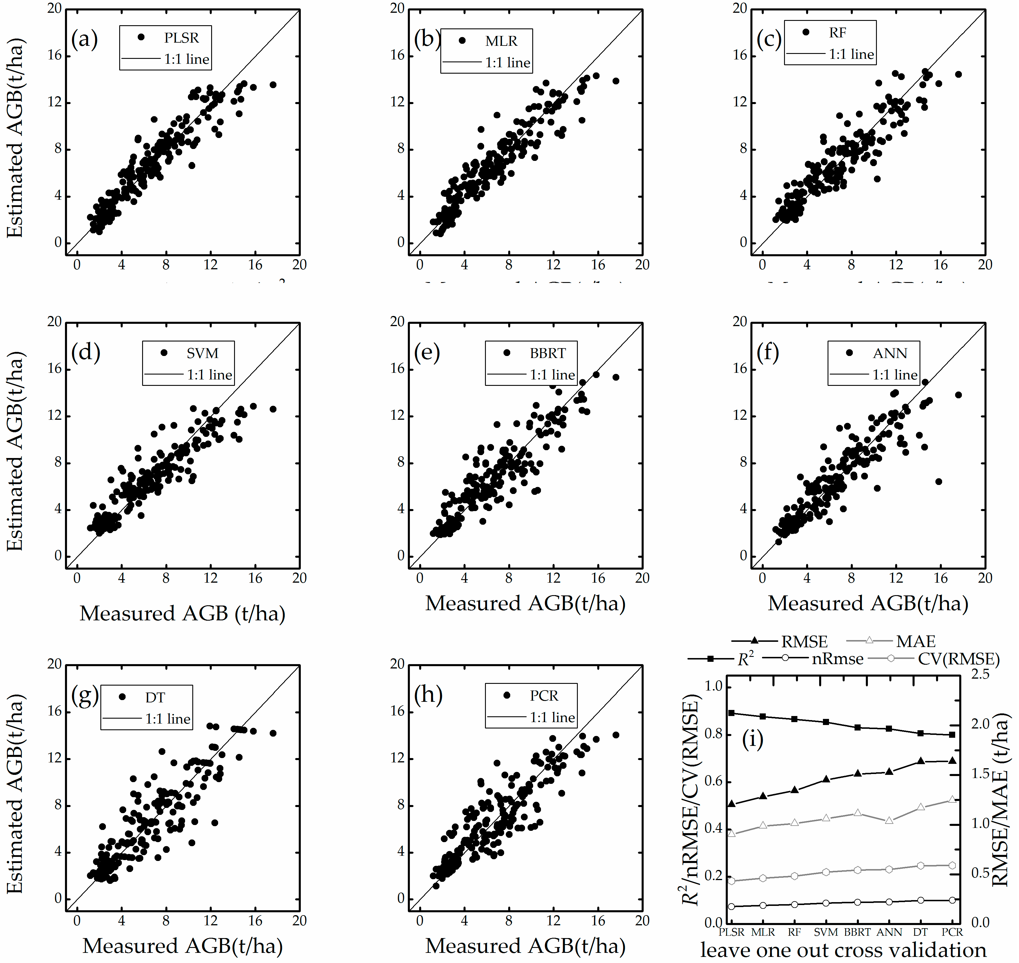
- Leave-one-out cross validation was used to evaluate the accuracy of the AGB estimation of these techniques (Section 4.4).
2. Materials
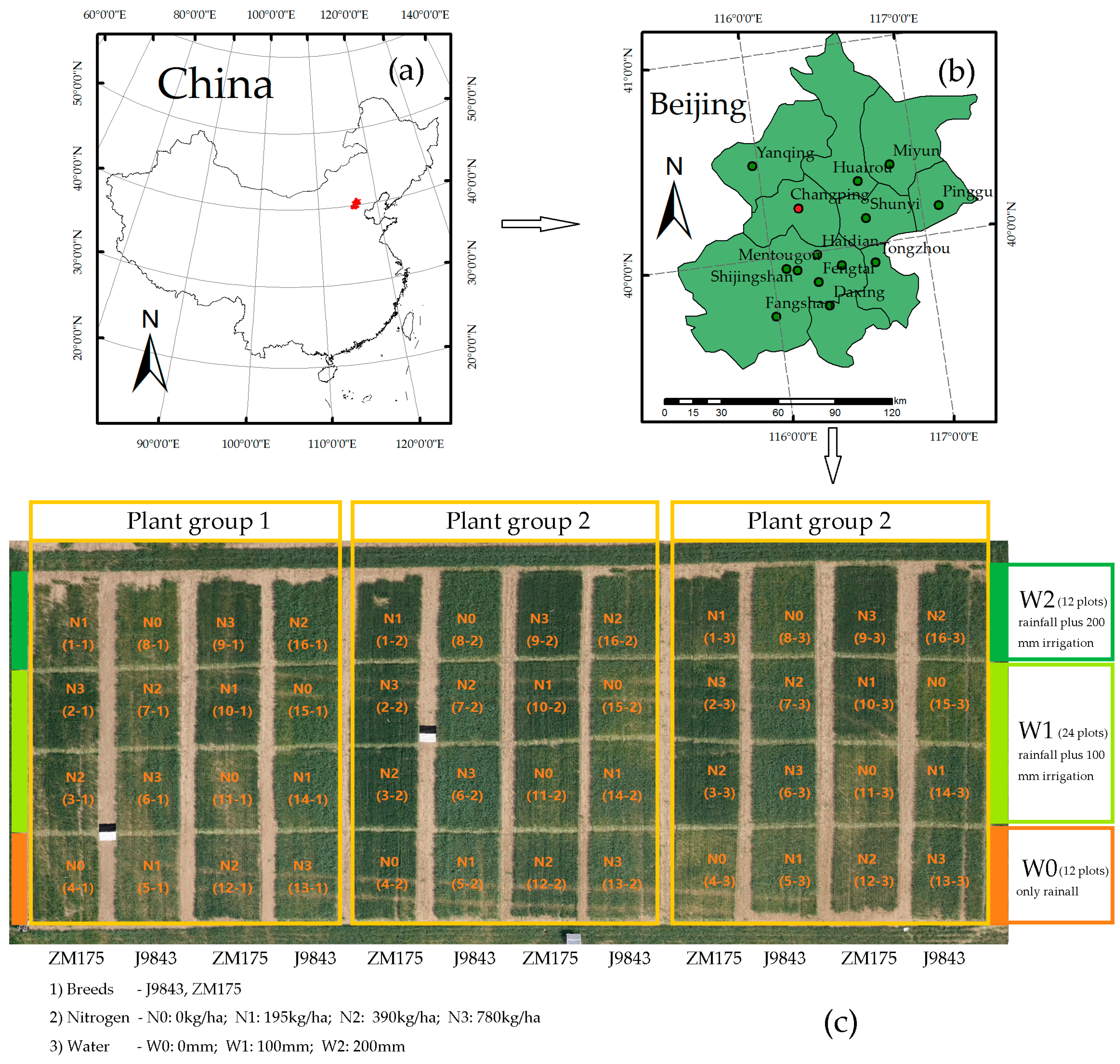
2.1. Study Area
2.2. Measurement of Data
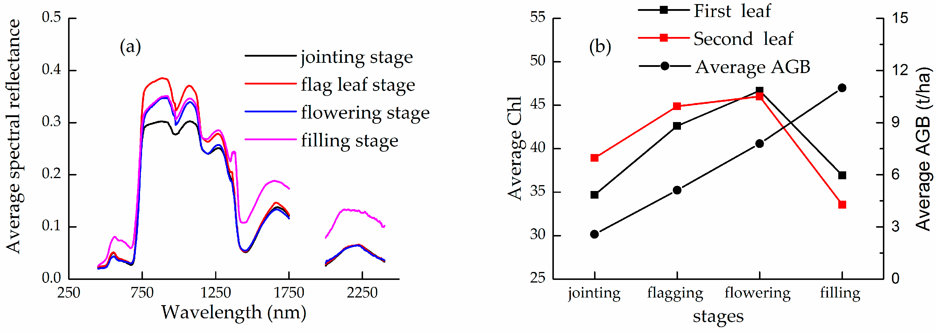
2.2.1. Measurements of Winter Wheat Canopy Reflectance
2.2.2. Measurements of Winter Wheat Chlorophyll and Above-Ground Biomass
3. Methods
3.1. Regression Techniques
3.1.1. Machine Learning Techniques
3.1.2. Conventional Regression Techniques
3.2. Selection of Vegetation Indexes
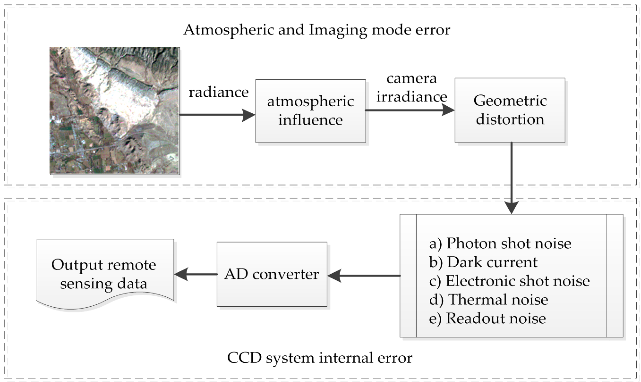
3.3. Noise Simulation
3.4. Modeling Parameters and Sampling Methods
3.5. Precision Evaluation
4. Results
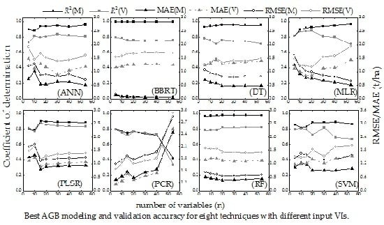
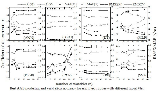
4.1. Selection of Vegetation Indexes
4.2. Test with White Gaussian Noise
4.3. Stability Test
4.4. Estimation Accuracy with Leave One Sampling
5. Analysis and Discussion
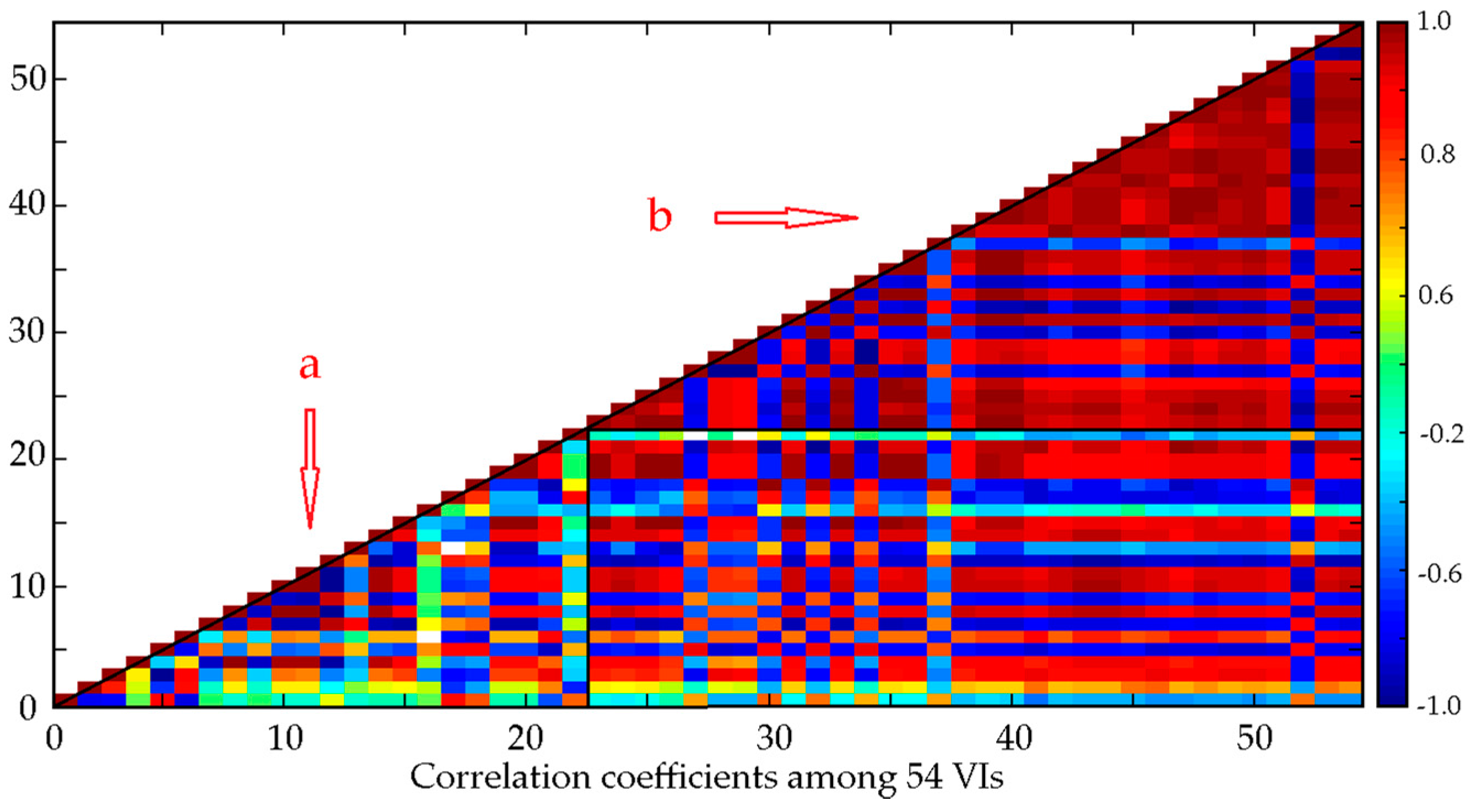
5.1. Analysis and Selection of Vegetation Indexes
5.2. Analysis of Noise Immunity
5.3. Analysis of Stability and Prediction Performance
6. Conclusions
- (1)
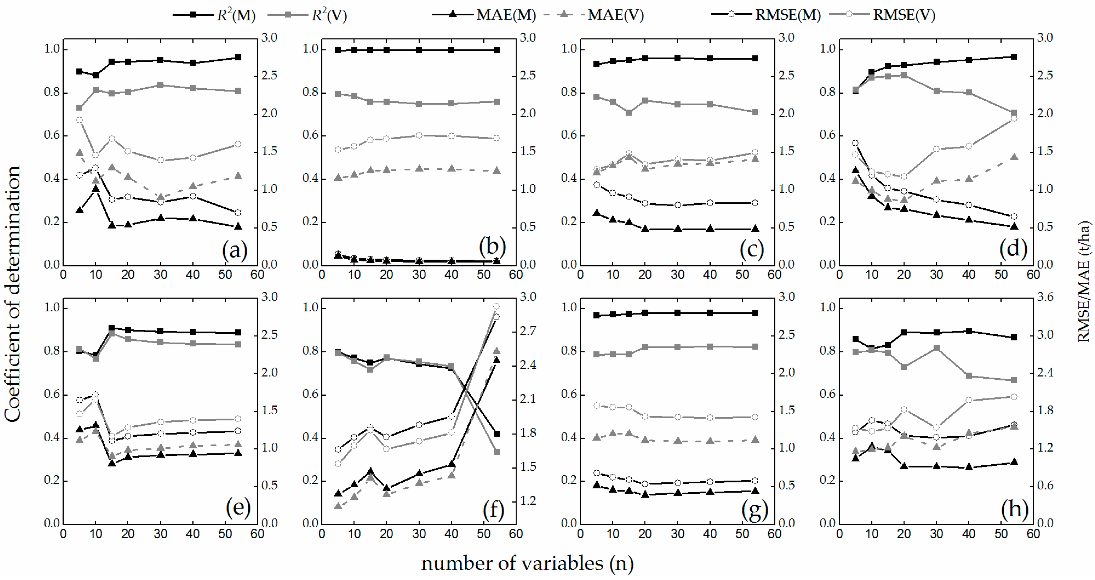
- Machine learning is the correct technique for tackling the multi-collinearity problem. ANN, BBRT and RF are almost unaffected by the multi-collinearity problem (Figure 6a,b,g), while MLR and PCR could not solve it.
- (2)
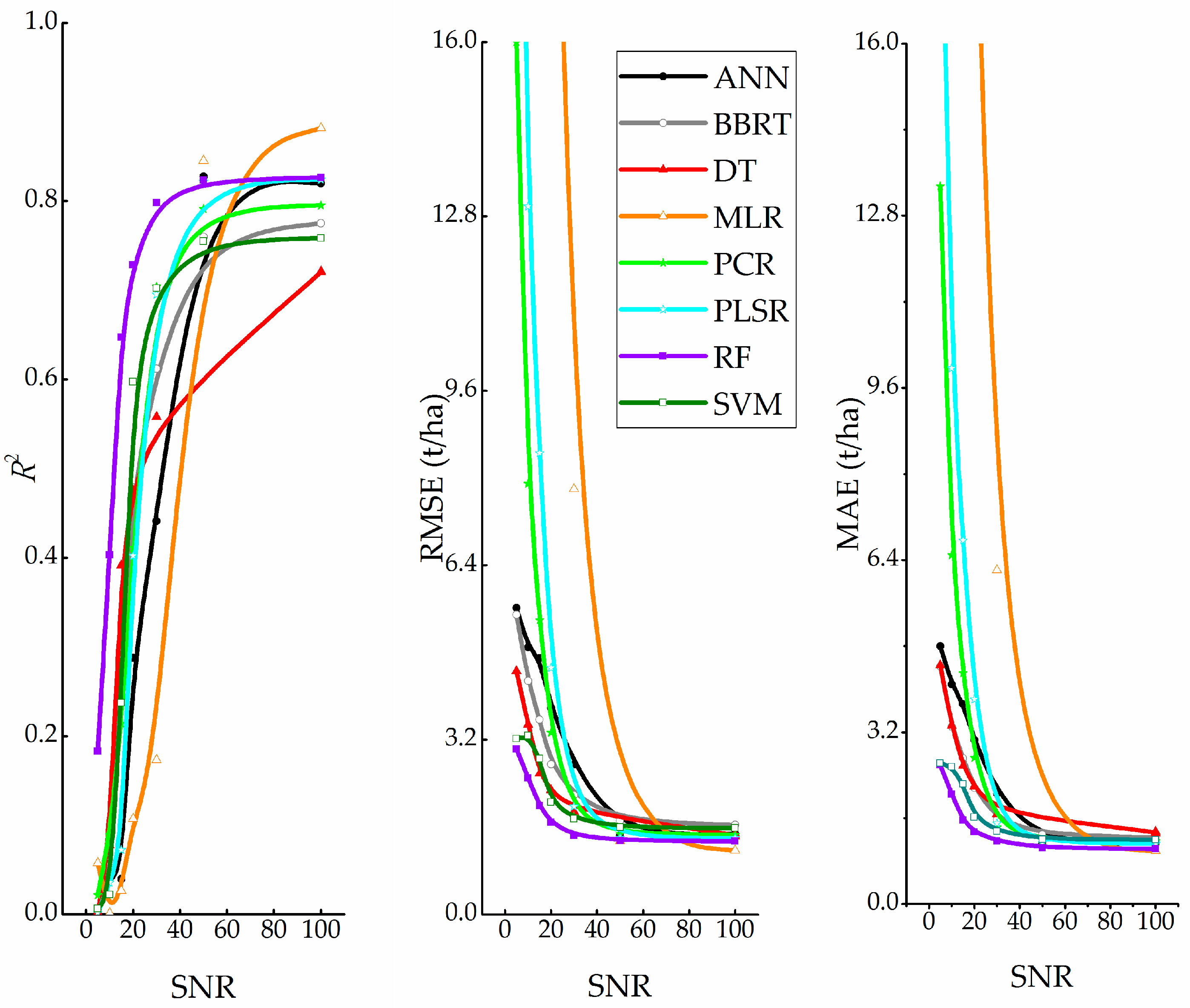
- Machine learning techniques are much more immune to noise than conventional regression techniques. In terms of noise immunity, the techniques are ranked as follows (Figure 7): RF > SVM >DT > BBRT >ANN > PCR > PLSR > MLR. Thus, RF may be suitable for work that requires repeated observations via remote sensing.
- (3)
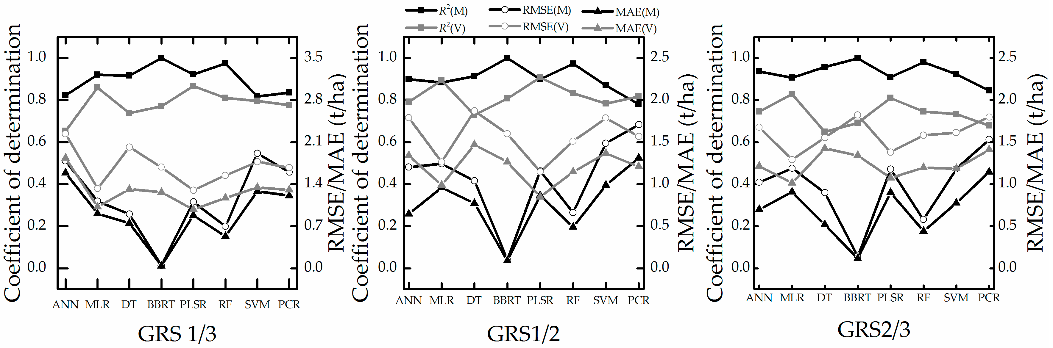
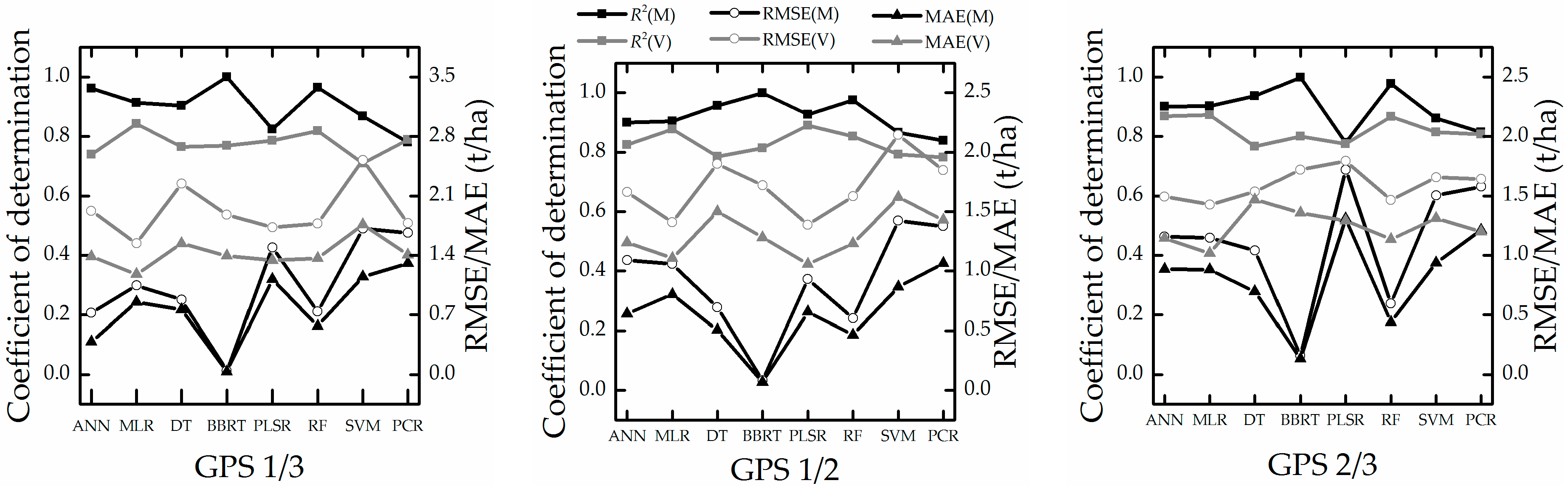
- The growth-period random sampling method performed better in stability tests. PLSR and MLR perform well in all stability tests (Figure 8 and Figure 9 and Table 6 and Table 7); these techniques and the sampling method may be suitable for work in which only a few samples are available for high-accuracy and stability estimation modeling.
- (4)
- This study demonstrated the potential application of VIs, machine learning and conventional regression techniques in estimating winter wheat biomass. The experimental results indicated that PLSR, MLR, and RF may be suitable for work that requires high-accuracy estimation models.
Acknowledgments
Author Contributions
Conflicts of Interest
Appendix A

| Component | 54VIs | 40VIs | 30VIs | 20VIs | 15VIs | 10VIs | 5VIs |
|---|---|---|---|---|---|---|---|
| 1 | 75.891 | 70.822 | 65.584 | 62.495 | 65.402 | 60.494 | 68.135 |
| 2 | 85.003 | 82.513 | 80.511 | 81.348 | 87.255 | 89.711 | 89.136 |
| 3 | 92.211 | 91.435 | 91.553 | 92.157 | 94.391 | 94.269 | 97.232 |
| 4 | 95.228 | 94.586 | 94.757 | 94.774 | 96.541 | 97.199 | 99.927 |
| 5 | 97.350 | 97.109 | 97.179 | 97.235 | 98.056 | 98.596 | 100.000 |
| 6 | 98.149 | 98.025 | 98.226 | 98.246 | 99.039 | 99.514 | - |
| 7 | 98.706 | 98.683 | 98.841 | 98.817 | 99.483 | 99.887 | - |
| 8 | 99.217 | 99.137 | 99.242 | 99.306 | 99.779 | 99.956 | - |
| 9 | 99.425 | 99.391 | 99.551 | 99.662 | 99.881 | 99.985 | - |
| 10 | 99.614 | 99.633 | 99.696 | 99.824 | 99.940 | 100.000 | - |
| 11 | 99.726 | 99.746 | 99.801 | 99.889 | 99.965 | - | - |
| 12 | 99.817 | 99.829 | 99.870 | 99.927 | 99.986 | - | - |
| 13 | 99.872 | 99.885 | 99.903 | 99.958 | 99.994 | - | - |
| 14 | 99.902 | 99.914 | 99.931 | 99.974 | 100.000 | - | - |
| 15 | 99.927 | 99.933 | 99.951 | 99.988 | 100.000 | - | - |
| 16 | 99.942 | 99.950 | 99.967 | 99.994 | - | - | - |
| 17 | 99.956 | 99.963 | 99.979 | 99.998 | - | - | - |
| 18 | 99.966 | 99.975 | 99.985 | 100.000 | - | - | - |
| 19 | 99.974 | 99.984 | 99.989 | 100.000 | - | - | - |
| 20 | 99.980 | 99.989 | 99.994 | 100.000 | - | - | - |
| 21 | 99.985 | 99.992 | 99.996 | - | - | - | - |
| 22 | 99.988 | 99.994 | 99.998 | - | - | - | - |
| 23 | 99.991 | 99.996 | 99.998 | - | - | - | - |
| 24 | 99.993 | 99.997 | 99.999 | - | - | - | - |
| 25 | 99.994 | 99.998 | 100.000 | - | - | - | - |
| 26 | 99.996 | 99.999 | 100.000 | - | - | - | - |
| 27 | 99.996 | 99.999 | 100.000 | - | - | - | - |
| 28 | 99.997 | 99.999 | 100.000 | - | - | - | - |
| 29 | 99.998 | 100.000 | 100.000 | - | - | - | - |
| 30 | 99.998 | 100.000 | 100.000 | - | - | - | - |
| 31 | 99.999 | 100.000 | - | - | - | - | - |
| 32 | 99.999 | 100.000 | - | - | - | - | - |
| 33 | 99.999 | 100.000 | - | - | - | - | - |
| 34 | 99.999 | 100.000 | - | - | - | - | - |
| 35 | 100.000 | 100.000 | - | - | - | - | - |
| 36 | 100.000 | 100.000 | - | - | - | - | - |
| 37 | 100.000 | 100.000 | - | - | - | - | - |
| 38 | 100.000 | 100.000 | - | - | - | - | - |
| 39 | 100.000 | 100.000 | - | - | - | - | - |
| 40 | 100.000 | 100.000 | - | - | - | - | - |
| 41 | 100.000 | - | - | - | - | - | - |
| 42 | 100.000 | - | - | - | - | - | - |
| 43 | 100.000 | - | - | - | - | - | - |
| 44 | 100.000 | - | - | - | - | - | - |
| 45 | 100.000 | - | - | - | - | - | - |
| 46 | 100.000 | - | - | - | - | - | - |
| 47 | 100.000 | - | - | - | - | - | - |
| 48 | 100.000 | - | - | - | - | - | - |
| 49 | 100.000 | - | - | - | - | - | - |
| 50 | 100.000 | - | - | - | - | - | - |
| 51 | 100.000 | - | - | - | - | - | - |
| 52 | 100.000 | - | - | - | - | - | - |
| 53 | 100.000 | - | - | - | - | - | - |
| 54 | 100.000 | - | - | - | - | - | - |
| VI | 54VIs | VI | 40VIs | VI | 30VIs | VI | 20VIs | VI | 15VIs | VI | 10VIs | VI | 5VIs |
|---|---|---|---|---|---|---|---|---|---|---|---|---|---|
| 1 | 121.3 | 1 | 84.0 | 1 | 46.6 | 1 | 35.0 | 1 | 20.7 | 1 | 13.7 | 1 | 7.1 |
| 2 | 793.8 | 2 | 400.9 | 2 | 323.2 | 2 | 28.3 | 2 | 7.2 | 2 | 6.0 | 2 | 3.3 |
| 3 | 1118.0 | 3 | 615.0 | 3 | 511.4 | 3 | 317.0 | 3 | 177.2 | 3 | 143.8 | 3 | 121.2 |
| 4 | 492.3 | 4 | 399.1 | 4 | 346.3 | 4 | 203.3 | 4 | 173.3 | 4 | 94.1 | 4 | 3.5 |
| 5 | 2673.3 | 5 | 2015.7 | 5 | 1492.1 | 5 | 471.6 | 5 | 258.9 | 5 | 215.0 | 5 | 150.6 |
| 6 | 16.2 | 6 | 14.0 | 6 | 13.9 | 6 | 11.7 | 6 | 9.1 | 6 | 6.5 | - | - |
| 7 | 1122.8 | 7 | 1526.1 | 7 | 1190.1 | 7 | 395.0 | 7 | 326.8 | 7 | 19.9 | - | - |
| 8 | 2441.3 | 8 | 1548.6 | 8 | 1290.8 | 8 | 1023.6 | 8 | 779.8 | 8 | 287.1 | - | - |
| 9 | 172.7 | 9 | 114.8 | 9 | 79.4 | 9 | 41.8 | 9 | 32.8 | 9 | 7.7 | - | - |
| 11 | 2138.9 | 11 | 1271.3 | 11 | 828.0 | 11 | 497.9 | 11 | 438.6 | 10 | 408.9 | - | - |
| 12 | 1637.2 | 12 | 1188.4 | 12 | 1133.6 | 12 | 805.6 | 12 | 616.8 | - | - | - | - |
| 13 | 358.1 | 13 | 1227.3 | 13 | 956.0 | 13 | 86.9 | 13 | 29.4 | - | - | - | - |
| 14 | 175.4 | 14 | 156.0 | 14 | 148.3 | 14 | 111.3 | 14 | 72.1 | - | - | - | - |
| 15 | 3285.7 | 15 | 3332.0 | 15 | 3899.8 | 15 | 1486.7 | 15 | 146.8 | - | - | - | - |
| 16 | 191.9 | 16 | 101.7 | 16 | 85.5 | 16 | 39.2 | - | - | - | - | - | - |
| 17 | 1130.6 | 17 | 1128.6 | 17 | 918.1 | 17 | 23.0 | - | - | - | - | - | - |
| 18 | 156.2 | 18 | 118.5 | 18 | 79.0 | 18 | 18.7 | - | - | - | - | - | - |
| 21 | 6258.6 | 21 | 3884.6 | 21 | 886.0 | 20 | 1280.1 | - | - | - | - | - | - |
| 22 | 663.8 | 22 | 572.1 | 22 | 470.4 | - | - | - | - | - | - | - | - |
| 24 | 996.9 | 24 | 706.2 | 24 | 207.5 | - | - | - | - | - | - | - | - |
| 25 | 3304.2 | 26 | 8495.2 | 26 | 2382.6 | - | - | - | - | - | - | - | - |
| 28 | 5845.4 | 27 | 2114.8 | 27 | 7627.7 | - | - | - | - | - | - | - | - |
| 30 | 1939.9 | 28 | 3010.1 | 28 | 1554.9 | - | - | - | - | - | - | - | - |
| 32 | 8499.5 | 30 | 1287.1 | 30 | 2371.2 | - | - | - | - | - | - | - | - |
| 34 | 3063.2 | 32 | 6092.3 | 32 | 177.4 | - | - | - | - | - | - | - | - |
| 37 | 59.0 | 37 | 42.0 | - | - | - | - | - | - | - | - | - | |
| 38 | 2705.9 | 38 | 148.6 | - | - | - | - | - | - | - | - | - | - |
| 41 | 4203.8 | 40 | 4259.2 | - | - | - | - | - | - | - | - | - | - |
| 45 | 4723.4 | - | - | - | - | - | - | - | - | - | - | - | - |
| 46 | 2086.8 | - | - | - | - | - | - | - | - | - | - | - | - |
| 50 | 4010.9 | - | - | - | - | - | - | - | - | - | - | - | - |
| 51 | 1151.1 | - | - | - | - | - | - | - | - | - | - | - | - |
| 52 | 4666.7 | - | - | - | - | - | - | - | - | - | - | - | - |
| 54 | 3874.4 | - | - | - | - | - | - | - | - | - | - | - | - |
References
- Wang, J.; Zhao, C.; Huang, W. Fundamental and Application of Quantitative Remote Sensing in Agriculture; Science China Press: Beijing, China, 2008. [Google Scholar]
- Jin, X.; Li, Z.; Yang, G.; Yang, H.; Feng, H.; Xu, X.; Wang, J.; Li, X.; Luo, J. Winter wheat yield estimation based on multi-source medium resolution optical and radar imaging data and the AquaCrop model using the particle swarm optimization algorithm. ISPRS J. Photogramm. Remote Sens. 2017, 126, 24–37. [Google Scholar] [CrossRef]
- Huang, J.; Sedano, F.; Huang, Y.; Ma, H.; Li, X.; Liang, S.; Tian, L.; Zhang, X.; Fan, J.; Wu, W. Assimilating a synthetic Kalman filter leaf area index series into the WOFOST model to improve regional winter wheat yield estimation. Agric. For. Meteorol. 2016, 216, 188–202. [Google Scholar] [CrossRef]
- Hensgen, F.; Bühle, L.; Wachendorf, M. The effect of harvest, mulching and low-dose fertilization of liquid digestate on above ground biomass yield and diversity of lower mountain semi-natural grasslands. Agric. Ecosyst. Environ. 2016, 216, 283–292. [Google Scholar] [CrossRef]
- Jin, X.; Kumar, L.; Li, Z.; Xu, X.; Yang, G.; Wang, J. Estimation of winter wheat biomass and yield by combining the aquacrop model and field hyperspectral data. Remote Sens. 2016, 8. [Google Scholar] [CrossRef]
- Boschetti, M.; Bocchi, S.; Brivio, P.A. Assessment of pasture production in the Italian Alps using spectrometric and remote sensing information. Agric. Ecosyst. Environ. 2007, 118, 267–272. [Google Scholar] [CrossRef]
- Atzberger, C.; Guérif, M.; Baret, F.; Werner, W. Comparative analysis of three chemometric techniques for the spectroradiometric assessment of canopy chlorophyll content in winter wheat. Comput. Electron. Agric. 2010, 73, 165–173. [Google Scholar] [CrossRef]
- Fu, Y.; Yang, G.; Wang, J.; Song, X.; Feng, H. Winter wheat biomass estimation based on spectral indices, band depth analysis and partial least squares regression using hyperspectral measurements. Comput. Electron. Agric. 2014, 100, 51–59. [Google Scholar] [CrossRef]
- Yue, J.; Yang, G.; Li, C.; Li, Z.; Wang, Y.; Feng, H.; Xu, B. Estimation of Winter Wheat Above-Ground Biomass Using Unmanned Aerial Vehicle-Based Snapshot Hyperspectral Sensor and Crop Height Improved Models. Remote Sens. 2017, 9, 708. [Google Scholar] [CrossRef]
- Atzberger, C.; Darvishzadeh, R.; Immitzer, M.; Schlerf, M.; Skidmore, A.; le Maire, G. Comparative analysis of different retrieval methods for mapping grassland leaf area index using airborne imaging spectroscopy. Int. J. Appl. Earth Obs. Geoinf. 2015, 43, 19–31. [Google Scholar] [CrossRef]
- Cho, M.A.; Skidmore, A.; Corsi, F.; van Wieren, S.E.; Sobhan, I. Estimation of green grass/herb biomass from airborne hyperspectral imagery using spectral indices and partial least squares regression. Int. J. Appl. Earth Obs. Geoinf. 2007, 9, 414–424. [Google Scholar] [CrossRef]
- Schlerf, M.; Atzberger, C.; Hill, J. Remote sensing of forest biophysical variables using HyMap imaging spectrometer data. Remote Sens. Environ. 2005, 95, 177–194. [Google Scholar] [CrossRef]
- Galvão, L.S.; Formaggio, A.R.; Tisot, D.A. Discrimination of sugarcane varieties in Southeastern Brazil with EO-1 Hyperion data. Remote Sens. Environ. 2005, 94, 523–534. [Google Scholar] [CrossRef]
- Wang, W. The Associations of Photosynthesis and Gain Filling during Grain Filling Period in Flag Leaves of Wheat Species; Ocean University of China: Qingdao, China, 2007. [Google Scholar]
- Datt, B. A New Reflectance Index for Remote Sensing of Chlorophyll Content in Higher Plants: Tests using Eucalyptus Leaves. J. Plant Physiol. 1999, 154, 30–36. [Google Scholar] [CrossRef]
- Broge, N.H.; Leblanc, E. Comparing prediction power and stability of broadband and hyperspectral vegetation indices for estimation of green leaf area index and canopy chlorophyll density. Remote Sens. Environ. 2001, 76, 156–172. [Google Scholar] [CrossRef]
- Sun, H.; Li, M.Z.; Zhao, Y.; Zhang, Y.E.; Wang, X.M.; Li, X.H. The Spectral Characteristics and Chlorophyll Content at Winter Wheat Growth Stages. Spectrosc. Spectr. Anal. 2010, 30, 192–196. [Google Scholar] [CrossRef]
- Thenkabail, P.S. Biophysical and yield information for precision farming from near-real-time and historical Landsat TM images. Int. J. Remote Sens. 2003, 24, 2879–2904. [Google Scholar] [CrossRef]
- Rivera, J.; Verrelst, J.; Delegido, J.; Veroustraete, F.; Moreno, J. On the Semi-Automatic Retrieval of Biophysical Parameters Based on Spectral Index Optimization. Remote Sens. 2014, 6, 4927–4951. [Google Scholar] [CrossRef]
- Atzberger, C. Object-based retrieval of biophysical canopy variables using artificial neural nets and radiative transfer models. Remote Sens. Environ. 2004, 93, 53–67. [Google Scholar] [CrossRef]
- Yue, J.; Yang, G.; Feng, H. Comparative of remote sensing estimation models of winter wheat biomass based on random forest algorithm. Nongye Gongcheng Xuebao/Trans. Chin. Soc. Agric. Eng. 2016, 32, 175–182. [Google Scholar] [CrossRef]
- Mirzaie, M.; Darvishzadeh, R.; Shakiba, A.; Matkan, A.A.; Atzberger, C.; Skidmore, A. Comparative analysis of different uni- and multi-variate methods for estimation of vegetation water content using hyper-spectral measurements. Int. J. Appl. Earth Obs. Geoinf. 2014, 26, 1–11. [Google Scholar] [CrossRef]
- Du, H.; Sun, X.; Han, N.; Mao, F. RS estimation of inventory parameters and carbon storage of Moso bamboo forest based on synergistic use of object-based image analysis and decision tree. Chin. J. Appl. Ecol. 2017, 28. [Google Scholar] [CrossRef]
- Friedman, J.H. Greedy function approximation: A gradient boosting machine. Ann. Stat. 2001, 29, 1189–1232. [Google Scholar] [CrossRef]
- Breiman, L. Random forests. Mach. Learn. 2001, 45, 5–32. [Google Scholar] [CrossRef]
- Ali, I.; Greifeneder, F.; Stamenkovic, J.; Neumann, M.; Notarnicola, C. Review of machine learning approaches for biomass and soil moisture retrievals from remote sensing data. Remote Sens. 2015, 7, 16398–16421. [Google Scholar] [CrossRef]
- Cheng, J.H.; Dai, Q.; Sun, D.W.; Zeng, X.A.; Liu, D.; Pu, H. Bin Applications of non-destructive spectroscopic techniques for fish quality and safety evaluation and inspection. Trends Food Sci. Technol. 2013, 34, 18–31. [Google Scholar] [CrossRef]
- Pan, L.; Li, H.C.; Deng, Y.J.; Zhang, F.; Chen, X.D.; Du, Q. Hyperspectral dimensionality reduction by tensor sparse and low-rank graph-based discriminant analysis. Remote Sens. 2017, 9. [Google Scholar] [CrossRef]
- Gomez, C.; Lagacherie, P.; Coulouma, G. Continuum removal versus PLSR method for clay and calcium carbonate content estimation from laboratory and airborne hyperspectral measurements. Geoderma 2008, 148, 141–148. [Google Scholar] [CrossRef]
- Blackburn, G.A.; Pitman, J.I. Biophysical controls on the directional spectral reflectance properties of bracken (Pteridium aquilinum) canopies: Results of a field experiment. Int. J. Remote Sens. 1999, 20, 2265–2282. [Google Scholar] [CrossRef]
- Jin, X.; Xu, X.; Song, X.; Li, Z.; Wang, J.; Guo, W. Estimation of leaf water content in winter wheat using grey relational analysis-partial least squares modeling with hyperspectral data. Agron. J. 2013, 105, 1385–1392. [Google Scholar] [CrossRef]
- Pu, R.; Gong, P. Hyperspectral Remote Sensing of Vegetation Bioparameters. In Advances in Environmental Remote Sensing; CRC Press: Boca Raton, FL, USA, 2011; Volume 4, pp. 101–142. ISBN 9781420091816. [Google Scholar]
- Thenkabail, P.S.; Smith, R.B.; De Pauw, E. Hyperspectral vegetation indices and their relationships with agricultural crop characteristics. Remote Sens. Environ. 2000, 71, 158–182. [Google Scholar] [CrossRef]
- Liang, L.; Di, L.; Zhang, L.; Deng, M.; Qin, Z.; Zhao, S.; Lin, H. Estimation of crop LAI using hyperspectral vegetation indices and a hybrid inversion method. Remote Sens. Environ. 2015, 165, 123–134. [Google Scholar] [CrossRef]
- Gevrey, M.; Dimopoulos, I.; Lek, S. Review and comparison of methods to study the contribution of variables in artificial neural network models. Ecol. Model. 2003, 160, 249–264. [Google Scholar] [CrossRef]
- Cortes, C.; Vapnik, V. Support-Vector Networks. Mach. Learn. 1995, 20, 273–297. [Google Scholar] [CrossRef]
- Chang, C.-C.; Lin, C.-J. Libsvm. ACM Trans. Intell. Syst. Technol. 2011, 2, 1–27. [Google Scholar] [CrossRef]
- Utgoff, P.E.; Corporation, C.; Street, W. Decision Tree Induction Based on Efficient Tree Restructuring. Mach. Learn. 1997, 29, 5–44. [Google Scholar] [CrossRef]
- Fakiola, M.; Mishra, A.; Rai, M.; Singh, S.P.; O’Leary, R.A.; Ball, S.; Francis, R.W.; Firth, M.J.; Radford, B.T.; Miller, E.N.; et al. Classification and regression tree and spatial analyses reveal geographic heterogeneity in genome wide linkage study of indian visceral leishmaniasis. PLoS ONE 2010, 5, e15807. [Google Scholar] [CrossRef] [PubMed]
- Wold, H. Estimation of principal components and related models by iterative least squares. In Multivariate Analysis; Academic Press: New York, NY, USA, 1966; pp. 1391–1420. ISBN 0471411256. [Google Scholar]
- Baret, F.; Guyot, G. Potentials and limits of vegetation indices for LAI and APAR assessment. Remote Sens. Environ. 1991, 35, 161–173. [Google Scholar] [CrossRef]
- Sims, D.A.; Gamon, J.A. Relationships between leaf pigment content and spectral reflectance across a wide range of species, leaf structures and developmental stages. Remote Sens. Environ. 2002, 81, 337–354. [Google Scholar] [CrossRef]
- Huete, A.; Didan, K.; Miura, T.; Rodriguez, E.P.; Gao, X.; Ferreira, L.G. Overview of the radiometric and biophysical performance of the MODIS vegetation indices. Remote Sens. Environ. 2002, 83, 195–213. [Google Scholar] [CrossRef]
- Jiang, Z.; Huete, A.R.; Didan, K.; Miura, T. Development of a two-band enhanced vegetation index without a blue band. Remote Sens. Environ. 2008, 112, 3833–3845. [Google Scholar] [CrossRef]
- Zarco-Tejada, P.J.; Berjón, A.; López-Lozano, R.; Miller, J.R.; Martín, P.; Cachorro, V.; González, M.R.; De Frutos, A. Assessing vineyard condition with hyperspectral indices: Leaf and canopy reflectance simulation in a row-structured discontinuous canopy. Remote Sens. Environ. 2005, 99, 271–287. [Google Scholar] [CrossRef]
- Peñuelas, J.; Gamon, J.A.; Fredeen, A.L.; Merino, J.; Field, C.B. Reflectance indices associated with physiological changes in nitrogen- and water-limited sunflower leaves. Remote Sens. Environ. 1994, 48, 135–146. [Google Scholar] [CrossRef]
- Delalieux, S.; Somers, B.; Hereijgers, S.; Verstraeten, W.W.; Keulemans, W.; Coppin, P. A near-infrared narrow-waveband ratio to determine Leaf Area Index in orchards. Remote Sens. Environ. 2008, 112, 3762–3772. [Google Scholar] [CrossRef]
- Barnes, J.D.; Balaguer, L.; Manrique, E.; Elvira, S.; Davison, A.W. A reappraisal of the use of DMSO for the extraction and determination of chlorophylls a and b in lichens and higher plants. Environ. Exp. Bot. 1992, 32, 85–100. [Google Scholar] [CrossRef]
- Qi, J.; Chehbouni, A.; Huete, A.R.; Kerr, Y.H.; Sorooshian, S. A modified soil adjusted vegetation index. Remote Sens. Environ. 1994, 48, 119–126. [Google Scholar] [CrossRef]
- Rama Rao, N.; Garg, P.K.; Ghosh, S.K.; Dadhwal, V.K. Estimation of leaf total chlorophyll and nitrogen concentrations using hyperspectral satellite imagery. J. Agric. Sci. 2008, 146, 65–75. [Google Scholar] [CrossRef]
- Chen, J.M. Evaluation of vegetation indices and a modified simple ratio for boreal applications. Can. J. Remote Sens. 1996, 22, 229–242. [Google Scholar] [CrossRef]
- Gamon, J.A.; Peñuelas, J.; Field, C.B. A narrow-waveband spectral index that tracks diurnal changes in photosynthetic efficiency. Remote Sens. Environ. 1992, 41, 35–44. [Google Scholar] [CrossRef]
- Haboudane, D.; Miller, J.R.; Pattey, E.; Zarco-Tejada, P.J.; Strachan, I.B. Hyperspectral vegetation indices and novel algorithms for predicting green LAI of crop canopies: Modeling and validation in the context of precision agriculture. Remote Sens. Environ. 2004, 90, 337–352. [Google Scholar] [CrossRef]
- Blackburn, G.A. Quantifying chlorophylls and carotenoids at leaf and canopy scales: An evaluation of some hyperspectral approaches. Remote Sens. Environ. 1998, 66, 273–285. [Google Scholar] [CrossRef]
- Chappelle, E.W.; Kim, M.S.; McMurtrey, J.E. Ratio analysis of reflectance spectra (RARS): An algorithm for the remote estimation of the concentrations of chlorophyll A, chlorophyll B, and carotenoids in soybean leaves. Remote Sens. Environ. 1992, 39, 239–247. [Google Scholar] [CrossRef]
- Rouse, J.W.; Hass, R.H.; Schell, J.A.; Deering, D.W. Monitoring vegetation systems in the great plains with ERTS. In Proceedings of the Third Earth Resources Technology Satellite Symposium, Washington, DC, USA, 10–14 December 1973; pp. 309–317. [Google Scholar]
- Gamon, J.A.; Surfus, J.S. Assessing leaf pigment content and activity with a reflectometer. New Phytol. 1999, 143, 105–117. [Google Scholar] [CrossRef]
- Rondeaux, G.; Steven, M.; Baret, F. Optimization of soil-adjusted vegetation indices. Remote Sens. Environ. 1996, 55, 95–107. [Google Scholar] [CrossRef]
- Penuelas, J.; Baret, F.; Filella, I. Semi-empirical indices to assess carotenoids/chlorophyll a ratio from leaf spectral reflectance. Photosynthetica 1995, 31, 221–230. [Google Scholar]
- Nagler, P.L.; Daughtry, C.S.T.; Goward, S.N. Plant litter and soil reflectance. Remote Sens. Environ. 2000, 71, 207–215. [Google Scholar] [CrossRef]
- Roujean, J.L.; Breon, F.M. Estimating PAR absorbed by vegetation from bidirectional reflectance measurements. Remote Sens. Environ. 1995, 51, 375–384. [Google Scholar] [CrossRef]
- Serrano, L.; Peñuelas, J.; Ustin, S.L. Remote sensing of nitrogen and lignin in Mediterranean vegetation from AVIRIS data: Decomposing biochemical from structural signals. Remote Sens. Environ. 2002, 81, 355–364. [Google Scholar] [CrossRef]
- Vincini, M.; Frazzi, E.; D’Alessio, P. Angular Dependence of Maize and Sugar Beet VIs from Directional CHRIS/Proba Data. Available online: https://www.researchgate.net/profile/Ermes_Frazzi/publication/228413259_Angular_dependence_of_maize_and_sugar_beet_VIs_from_directional_CHRISProba_data/links/0046352d50c18b3fe6000000.pdf (accessed on 3 January 2018).
- Haboudane, D.; Miller, J.R.; Tremblay, N.; Zarco-Tejada, P.J.; Dextraze, L. Integrated narrow-band vegetation indices for prediction of crop chlorophyll content for application to precision agriculture. Remote Sens. Environ. 2002, 81, 416–426. [Google Scholar] [CrossRef]
- Jordan, C.F. Derivation of Leaf-Area Index from Quality of Light on the Forest Floor. Source Ecol. 1969, 50, 663–666. [Google Scholar] [CrossRef]
- Gitelson, A.A.; Kaufman, Y.J.; Stark, R.; Rundquist, D. Novel algorithms for remote estimation of vegetation fraction. Remote Sens. Environ. 2002, 80, 76–87. [Google Scholar] [CrossRef]
- Hunt, E.R.; Rock, B.N. Detection of changes in leaf water content using Near- and Middle-Infrared reflectances. Remote Sens. Environ. 1989, 30, 43–54. [Google Scholar] [CrossRef]
- Stamatiadis, S.; Taskos, D.; Tsadilas, C.; Christofides, C.; Tsadila, E.; Schepers, J.S. Relation of ground-sensor canopy reflectance to biomass production and grape color in two merlot vineyards. Am. J. Enol. Vitic. 2006, 57, 415–422. [Google Scholar] [CrossRef]
- Hardisky, M.A.; Klemas, V.; Smart, R.M. The influence of Soil Salinity, Growth Form, and Leaf Moisture on the Spectral Radiance of Spartina alterniflora Canopies. Photogramm. Eng. Remote Sens. 1983, 49, 77–83. [Google Scholar]
- Gitelson, A.A.; Merzlyak, M.N.; Chivkunova, O.B. Optical Properties and Nondestructive Estimation of Anthocyanin Content in Plant Leaves. Photochem. Photobiol. 2001, 74, 38–45. [Google Scholar] [CrossRef]
- Datt, B.; McVicar, T.R.; Van Niel, T.G.; Jupp, D.L.B.; Pearlman, J.S. Preprocessing EO-1 Hyperion hyperspectral data to support the application of agricultural indexes. IEEE Trans. Geosci. Remote Sens. 2003, 41, 1246–1259. [Google Scholar] [CrossRef]
- Fensholt, R.; Sandholt, I. Derivation of a shortwave infrared water stress index from MODIS near- and shortwave infrared data in a semiarid environment. Remote Sens. Environ. 2003, 87, 111–121. [Google Scholar] [CrossRef]
- Zarco-Tejada, P.J.; Rueda, C.A.; Ustin, S.L. Water content estimation in vegetation with MODIS reflectance data and model inversion methods. Remote Sens. Environ. 2003, 85, 109–124. [Google Scholar] [CrossRef]
- Daughtry, C.S.T.; Walthall, C.L.; Kim, M.S.; De Colstoun, E.B.; McMurtrey, J.E. Estimating corn leaf chlorophyll concentration from leaf and canopy reflectance. Remote Sens. Environ. 2000, 74, 229–239. [Google Scholar] [CrossRef]
- Penuelas, J.; Pinol, J.; Ogaya, R.; Filella, I. Estimation of plant water concentration by the reflectance Water Index WI (R900/R970). Int. J. Remote Sens. 1997, 18, 2869–2875. [Google Scholar] [CrossRef]
- Merzlyak, M.N.; Gitelson, A.A.; Chivkunova, O.B.; Rakitin, V.Y.U. Non-destructive optical detection of pigment changes during leaf senescence and fruit ripening. Physiol. Plant. 1999, 106, 135–141. [Google Scholar] [CrossRef]
- Merton, R.; Huntington, J. Early Simulation Results of the Aries-1 Satellite Sensor for Multi-Temporal Vegetation Research Derived from Aviris. In Proceedings of the Eighth Annual JPL Airborne Earth Science Workshop, Pasadena, CA, USA, 9–11 February 1999; pp. 1–10. [Google Scholar]
- Matsushita, Y.; Lin, S. Radiometric calibration from noise distributions. In Proceedings of the IEEE Conference on Computer Vision and Pattern Recognition, Minneapolis, MN, USA, 17–22 June 2007. [Google Scholar] [CrossRef]
- Tsin, Y.; Ramesh, V.; Kanade, T. Statistical calibration of CCD imaging process. In Proceedings of the Eighth IEEE International Conference on Computer Vision, Vancouver, BC, Canada, 7–14 July 2001; pp. 480–487. [Google Scholar] [CrossRef]
- You, H.; Ma, Z.; Tang, Y.; Wang, Y.; Yan, J.; Ni, M.; Cen, K.; Huang, Q. Comparison of ANN (MLP), ANFIS, SVM, and RF models for the online classification of heating value of burning municipal solid waste in circulating fluidized bed incinerators. Waste Manag. 2016. [Google Scholar] [CrossRef] [PubMed]
- Yuan, H.; Yang, G.; Li, C.; Wang, Y.; Liu, J.; Yu, H.; Feng, H.; Xu, B.; Zhao, X.; Yang, X. Retrieving soybean leaf area index from unmanned aerial vehicle hyperspectral remote sensing: Analysis of RF, ANN, and SVM regression models. Remote Sens. 2017, 9. [Google Scholar] [CrossRef]
- Cochran, W.G. Sampling Technique; China Statistical Publishing House: Beijing, China, 1985. [Google Scholar]
- Volpe, V.; Manzoni, S.; Marani, M.; Katul, G. Leave-One-Out Cross-Validation; Springer: Berlin, Germany, 2011. [Google Scholar]
- Humbeck, K.; Quast, S.; Krupinska, K. Functional and molecular changes in the photosynthetic apparatus during senescence of flag leaves from field-grown barley plants. Plant Cell Environ. 1996, 19, 337–344. [Google Scholar] [CrossRef]
- Martínez-Muñoz, G.; Suárez, A. Out-of-bag estimation of the optimal sample size in bagging. Pattern Recognit. 2010, 43, 143–152. [Google Scholar] [CrossRef]
- Garg, A.; Kang, T.; Tai, K. Comparison of statistical and machine learning methods in modelling of data with multicollinearity. Int. J. Model. Identif. Control 2013, 18, 295–312. [Google Scholar] [CrossRef]
- Abdullah, S.; Ismail, M.; Fong, S.Y.; Ahmed, A.M.A.N. Evaluation for long term PM10 concentration forecasting using multi linear regression (MLR) and principal component regression (PCR) models. Environ. Asia 2016, 9, 101–110. [Google Scholar]
- Jin, X.; Ma, J.; Wen, Z.; Song, K. Estimation of maize residue cover using Landsat-8 OLI image spectral information and textural features. Remote Sens. 2015, 7, 14559–14575. [Google Scholar] [CrossRef]
- Altmann, A.; Toloşi, L.; Sander, O.; Lengauer, T. Permutation importance: A corrected feature importance measure. Bioinformatics 2010, 26, 1340–1347. [Google Scholar] [CrossRef] [PubMed]
- Deng, H.; Runger, G.; Tuv, E. Bias of importance measures for multi-valued attributes and solutions. In Proceedings of the 21st International Conference on Articial Neural Networks (ICANN 2011), Espoo, Finland, 14–17 June 2011; pp. 293–300. [Google Scholar]
- Zhao, W.; Hopke, P.K.; Qin, X.; Prather, K.A. Predicting bulk ambient aerosol compositions from ATOFMS data with ART-2a and multivariate analysis. Anal. Chim. Acta 2005, 549, 179–187. [Google Scholar] [CrossRef]
- Farifteh, J.; Van der Meer, F.; Atzberger, C.; Carranza, E.J.M. Quantitative analysis of salt-affected soil reflectance spectra: A comparison of two adaptive methods (PLSR and ANN). Remote Sens. Environ. 2007, 110, 59–78. [Google Scholar] [CrossRef]


| Period | Sample | Min (t/ha) | Max (t/ha) | Mean (t/ha) | Standard Deviation (t/ha) | Coefficient of Variation (%) |
|---|---|---|---|---|---|---|
| Jointing | 48 | 1.201 | 4.526 | 2.569 | 0.685 | 26.664 |
| Flag | 48 | 2.194 | 8.266 | 5.114 | 1.468 | 28.706 |
| Flowering | 48 | 3.419 | 12.737 | 7.790 | 1.960 | 25.160 |
| Grain filling | 48 | 5.456 | 17.599 | 10.993 | 2.793 | 25.407 |
| VIs | Equation | Reference | VIs | Equation | Reference |
|---|---|---|---|---|---|
| ATSAVI | a (R800 − a R670 − b)/[(a R800 + R670 − ab + X(1 + a2)], where X = 0.08, a = 1.22, and b = 0.03 | [41] | MND680 | (R800 − R680)/(R800 + R680 − 2R445) | [42] |
| EVI | 2.5(RNIR – RRed)/(RNIR + 6RRed − 7.5RBlue + 1) | [43] | MND705 | (R750 − R705)/(R750 + R705 − 2R445) | [42] |
| EVI2 | 2.5(RNIR − RRed)/(RNIR + 2.4RRed + 1) | [44] | MSR705 | (R750 − R445)/(R705 − R445) | [42] |
| GI | R554/R677 | [45] | NPCI | (R680 − R430)/(R680 + R430) | [46] |
| LAIDI | R1250/R1050 | [47] | NPQI | (R415 − R435)/(R415 + R435) | [48] |
| MSAVI | 0.5[2R800 + 1 − ((2R800 + 1)2 − 8(R800 − R670))1/2] | [49] | PBI | R810/R560 | [50] |
| MSR | (R800/R670 − 1)/(R800/R670 + 1)1/2 | [51] | PRI | (R531 − R570)/(R531 + R570) | [52] |
| MTVI1 | 1.2[1.2(R800 − R550) − 2.5(R670 − R550)] | [53] | PSSR | R800/R500 | [54] |
| MTVI2 | {1.5[1.2(R800 − R550) − 2.5(R670 − R550)]}/ {(2R800 + 1)2 − [6R800 − 5(R670)1/2] − 0.5}1/2 | [53] | RARS | R760/R500 | [55] |
| NDVI | (RNIR − RRed)/(RNIR + RRed) | [56] | RGR | RRed/RGreen | [57] |
| OSAVI | 1.16(R800 − R670)/(R800 + R670 + 0.16) | [58] | SIPI | (R800 − R445)/(R800 − R680) | [59] |
| PSND | (R800 − R470)/(R800 + R470) | [54] | TVI | 0.5[120(R750 − R550) − 200(R670 − R550)] | [16] |
| PVIhyp | (R1148 – a R807 − b)/(1 + a2)1/2, where a = 1.17 and b = 3.37 | [12] | CAI | 0.5(R2020 + R2220) − R2100 | [60] |
| RDVI | (R800 − R670)/(R800 + R670)1/2 | [61] | NDLI | [log(1/R1754) − log(1/R1680)] /[log(1/R1754) + log(1/R1680)] | [62] |
| SLAIDI | S(R1050 − R1250)/(R1050 + R1250), where S = 5 | [47] | NDNI | [log(1/R1510) − log(1/R1680)] /[log(1/R1510) + log(1/R1680)] | [62] |
| SPVI | 0.4[3.7(R800 − R670) − 1.2|R530 − R670|] | [63] | DSWI | (R802 + R547)/(R1657 + R682) | [13] |
| TCARI | 3[(R700 − R670) − 0.2(R700 − R550)(R700/R670)] | [64] | LWVI1 | (R1094 − R893)/(R1094 + R893) | [13] |
| SR | RNIR /RRed | [65] | LWVI2 | (R1094 − R1205)/(R1094 + R1205) | [13] |
| VARIgreen | (RGreen − RRed)/(RGreen + RRed) | [66] | MSI | R1600/R819 | [67] |
| WDRVI | (0.1 RNIR − RRed)/(0.1 RNIR + RRed) | [68] | NDII | (R819 − R1600)/(R819 + R1600) | [69] |
| ARI | (R550)−1 − (R700)−1 | [70] | NDWI | (R860 − R1240)/(R860 + R1240) | [71] |
| BGI | R450/R550 | [45] | RVIhyp | R1088/R1148 | [12] |
| BRI | R450/R690 | [45] | SIWSI | (R860 − R1640)/(R860 + R1640) | [72] |
| LCI | (R850 − R710)/(R850 + R680) | [15] | SRWI | R860/R1240 | [73] |
| MCARI | [(R701 − R671) − 0.2(R701 − R549)]/(R701/R671) | [74] | WI | R900/R970 | [75] |
| MCARI1 | 1.2[2.5(R800 − R670) − 1.3(R800 − R550)] | [53] | PSRI | (R680 − R500)/R750 | [76] |
| MCARI2 | {1.5[2.5(R800 − R670) − 1.3(R800 − R550)]} /{(2R800 + 1)2 − [6R800 − 5(R670)1/2] − 0.5}1/2 | [53] | RVSI | [(R712 + R752)/2] − R732 | [77] |
| Method | ANN | RF | SVM | ||||||||
|---|---|---|---|---|---|---|---|---|---|---|---|
| Parameters | Hidden layer 1 | Hidden layer 2 | SL | ntree | SL | mtry | SL | c | SL | g | SL |
| Min value | 1 | 1 | 1 | 0 | 20 | 1 | 1 | −10 | 0.5 | −10 | 0.5 |
| Max value | 20 | 20 | 2000 | 10 | 10 | 10 | |||||
| Number | VI | r | Number | VI | r | Number | VI | r |
|---|---|---|---|---|---|---|---|---|
| 1 | NPQI | 0.757 ** | 19 | MCARI1 | 0.226 ** | 37 | NDLI | 0.106 n.s. |
| 2 | BGI | 0.555 ** | 20 | MTVI1 | 0.226 ** | 38 | PSSR | 0.102 n.s. |
| 3 | BRI | 0.519 ** | 21 | MND680 | 0.193 ** | 39 | ATSAVI | 0.092 n.s. |
| 4 | RVIhyp | 0.490 ** | 22 | TCARI | 0.188 ** | 40 | OSAVI | 0.088 n.s. |
| 5 | NPCI | 0.474 ** | 23 | EVI2 | 0.182 * | 41 | MND705 | 0.086 n.s. |
| 6 | CAI | 0.442 ** | 24 | PSND | 0.180 * | 42 | RARS | 0.079 n.s. |
| 7 | PVIhyp | 0.370 ** | 25 | MSAVI | 0.180 * | 43 | SIWSI | 0.075 n.s. |
| 8 | LWVI2 | 0.352 ** | 26 | TVI | 0.177 * | 44 | NDWI | 0.075 n.s. |
| 9 | LWVI1 | 0.337 ** | 27 | GI | 0.176 * | 45 | PBI | 0.067 n.s. |
| 10 | SLAIDI | 0.304 ** | 28 | PRI | 0.176 * | 46 | MSR705 | 0.061 n.s. |
| 11 | SRWI | 0.300 ** | 29 | VARIgreen | 0.165 * | 47 | NDVI | 0.039 n.s. |
| 12 | LAIDI | 0.397 ** | 30 | SIPI | 0.157 * | 48 | LCI | 0.034 n.s. |
| 13 | RVSI | 0.299 ** | 31 | MCARI2 | 0.149 * | 49 | MSR | 0.032 n.s. |
| 14 | WI | 0.260 ** | 32 | PSRI | 0.149 * | 50 | WDRVI | 0.031 n.s. |
| 15 | SPVI | 0.251 ** | 33 | RDVI | 0.146 * | 51 | SR | 0.029 n.s. |
| 16 | ARI | 0.241 ** | 34 | RGR | 0.142 * | 52 | MSI | 0.029 n.s. |
| 17 | MCARI | 0.237 ** | 35 | EVI | 0.149 * | 53 | DSWI | 0.027 n.s. |
| 18 | NDNI | 0.228 ** | 36 | MTVI2 | 0.121 * | 54 | NDII | 0.012 n.s. |
| Technique | ANN | BBRT | DT | MLR | PLSR | PCR | RF | SVM |
|---|---|---|---|---|---|---|---|---|
| Number of input VIs | 30 | 5 | 5 | 20 | 15 | 5 | 30 | 30 |
| Technique | ∇R2 | ∇RMSE (t/ha) | ∇MAE (t/ha) | ||||||
|---|---|---|---|---|---|---|---|---|---|
| 1/3 | 1/2 | 2/3 | 1/3 | 1/2 | 2/3 | 1/3 | 1/2 | 2/3 | |
| ANN | 0.17 * | 0.11 | 0.19 * | 0.45 | 0.59 | 0.65 | 0.25 | 0.69 | 0.52 |
| MLR | 0.06 | 0.01 | 0.08 | 0.21 | 0.02 | 0.10 | 0.11 | 0.03 | 0.10 |
| DT | 0.18* | 0.18* | 0.31 * | 1.12 * | 0.83 * | 0.66 | 0.56 | 0.70 | 0.91 * |
| BBRT | 0.23 * | 0.19* | 0.31 * | 1.64 * | 1.49 * | 1.68 * | 1.23 * | 1.17 * | 1.23 * |
| PLSR | 0.05 | 0.01 | 0.10 | 0.19 | 0.01 | 0.20 | 0.10 | 0.02 | 0.17 |
| RF | 0.16* | 0.14 | 0.24 * | 0.85 * | 0.85* | 1.00 * | 0.64 | 0.66 | 0.76 |
| SVM | 0.02 | 0.09 | 0.19 * | 0.14 | 0.30 | 0.43 | 0.06 | 0.38 | 0.41 |
| PCR | 0.06 | 0.04 | 0.17 * | 0.07 | 0.14 | 0.26 | 0.10 | 0.11 | 0.26 |
| Technique | ∇R2 | ∇RMSE (t/ha) | ∇MAE (t/ha) | ||||||
|---|---|---|---|---|---|---|---|---|---|
| 1/3 | 1/2 | 2/3 | 1/3 | 1/2 | 2/3 | 1/3 | 1/2 | 2/3 | |
| ANN | 0.22 * | 0.07 | 0.03 | 1.20 * | 0.57 | 0.34 | 1.00 * | 0.60 | 0.26 |
| MLR | 0.07 | 0.03 | 0.03 | 0.50 | 0.35 | 0.28 | 0.32 | 0.30 | 0.14 |
| DT | 0.14 | 0.17 * | 0.17 * | 1.37 * | 1.20 * | 0.50 | 0.78 | 1.00 * | 0.77 |
| BBRT | 0.23 * | 0.19 * | 0.20 * | 1.83 * | 1.64 * | 1.56 * | 1.36 * | 1.21 * | 1.23 * |
| PLSR | 0.04 | 0.04 | 0.00 | 0.23 | 0.46 | 0.07 | 0.22 | 0.40 | 0.02 |
| RF | 0.14 | 0.12 | 0.11 | 1.04 * | 1.03 * | 0.87 * | 0.80 * | 0.77 | 0.70 |
| SVM | 0.16 * | 0.07 | 0.05 | 0.81 * | 0.72 | 0.15 | 0.62 | 0.76 | 0.37 |
| PCR | 0.01 | 0.06 | 0.01 | 0.11 | 0.47 | 0.06 | 0.10 | 0.36 | 0.01 |
© 2018 by the authors. Licensee MDPI, Basel, Switzerland. This article is an open access article distributed under the terms and conditions of the Creative Commons Attribution (CC BY) license (http://creativecommons.org/licenses/by/4.0/).
Share and Cite
Yue, J.; Feng, H.; Yang, G.; Li, Z. A Comparison of Regression Techniques for Estimation of Above-Ground Winter Wheat Biomass Using Near-Surface Spectroscopy. Remote Sens. 2018, 10, 66. https://doi.org/10.3390/rs10010066
Yue J, Feng H, Yang G, Li Z. A Comparison of Regression Techniques for Estimation of Above-Ground Winter Wheat Biomass Using Near-Surface Spectroscopy. Remote Sensing. 2018; 10(1):66. https://doi.org/10.3390/rs10010066
Chicago/Turabian StyleYue, Jibo, Haikuan Feng, Guijun Yang, and Zhenhai Li. 2018. "A Comparison of Regression Techniques for Estimation of Above-Ground Winter Wheat Biomass Using Near-Surface Spectroscopy" Remote Sensing 10, no. 1: 66. https://doi.org/10.3390/rs10010066
APA StyleYue, J., Feng, H., Yang, G., & Li, Z. (2018). A Comparison of Regression Techniques for Estimation of Above-Ground Winter Wheat Biomass Using Near-Surface Spectroscopy. Remote Sensing, 10(1), 66. https://doi.org/10.3390/rs10010066