Article

An Empirical Algorithm for Estimating Agricultural and Riparian Evapotranspiration Using MODIS Enhanced Vegetation Index and Ground Measurements of ET. I. Description of Method

1
US Geological Survey, Southwest Biological Science Center, Sonoran Desert Research Station, 1110 E. South Campus Drive, Room 123, Tucson, AZ 85721, USA
2
Laboratory of Tree Ring Research, 105 West Stadium, University of Arizona, Tucson, AZ 85721, USA
3
Environmental Research Laboratory, University of Arizona, 2601 East Airport Drive, Tucson, AZ 85706, USA
4
US Bureau of Reclamation, Denver Federal Center, Denver, CO 80225, USA
*
Author to whom correspondence should be addressed.
Remote Sens. 2009, 1(4), 1273-1297; https://doi.org/10.3390/rs1041273
Submission received: 13 October 2009 / Revised: 19 November 2009 / Accepted: 3 December 2009 / Published: 10 December 2009
(This article belongs to the Special Issue Global Croplands)

Abstract

:
We used the Enhanced Vegetation Index (EVI) from MODIS to scale evapotranspiration (ETactual) over agricultural and riparian areas along the Lower Colorado River in the southwestern US. Ground measurements of ETactual by alfalfa, saltcedar, cottonwood and arrowweed were expressed as fraction of potential (reference crop) ETo (EToF) then regressed against EVI scaled between bare soil (0) and full vegetation cover (1.0) (EVI*). EVI* values were calculated based on maximum and minimum EVI values from a large set of riparian values in a previous study. A satisfactory relationship was found between crop and riparian plant EToF and EVI*, with an error or uncertainty of about 20% in the mean estimate (mean ETactual = 6.2 mm d−1, RMSE = 1.2 mm d−1). The equation for ETactual was: ETactual = 1.22 × ETo-BC × EVI*, where ETo-BC is the Blaney Criddle formula for ETo. This single algorithm applies to all the vegetation types in the study, and offers an alternative to ETactual estimates that use crop coefficients set by expert opinion, by using an algorithm based on the actual state of the canopy as determined by time-series satellite images.

1. Introduction

1.1. The Vegetation Index Approach for Scaling ET by Remote Sensing

Recent studies have combined ground measurements of evapotranspiration (ET), meteorological variables, and vegetation indices (VIs) determined by satellite sensors to project plant water use over diverse biomes, including deserts [1,2], semiarid rangelands [3], agricultural districts [4,5,6], riparian corridors [7,8], rainforests [9], and mixed landscape units at regional [10,11] and global [12,13] scales of measurement. Unlike remote sensing methods based on thermal (NIR) bands on Landsat or other high-resolution satellites, which provide a snap-shot of actual ET (ETactual) at the time of satellite overpass [14,15], VI methods are useful in projecting ETactual over longer time periods (weeks, months and years), due to the modulated response of VIs to environmental conditions. These methods use time-series images from frequent-return sensor systems such as the Moderate Resolution Imaging Spectrometer (MODIS) on the Terra satellite [16,17].
VI methods work due to the high correlation between plant transpiration and green foliage density measured by VIs [16,17]. Unlike thermal-band methods, VI methods cannot estimate the direct evaporation component of ETactual [6]. However, in many biomes, plant transpiration dominates ETactual, and is often the major unknown in wide-area water budgets. In arid zone phreatophyte communities, as studied here, plants withdraw water from the underlying aquifer, precipitation is low, and the top meter of soil is often dry [1,7,8]. Bare soil evaporation is often a small term in the water budget of these systems.
Although many variations exist, most of the methods are based on initial observations by Choudhury et al. [18] who showed that crop transpiration on a ground area basis (EG) can be calculated as:
EG = ETo × k × VI*
where ETo is daily potential or reference crop ET determined from micrometeorological data from one of several possible methods, VI* is one of several possible VIs scaled between 0 (no vegetation) and 1 (full cover vegetation), and k is a constant determined by linear regression of measured EG with VI* over a crop cycle. Equation (1) can be rearranged to give the evaporative fraction (EGF), the ratio of EG to ETo:
EToF = EG / ETo = k × VI*
EToF can then be used to scale EG (e.g., from sap flow sensors) or ETactual (e.g., from moisture flux towers) over wider areas and longer time spans than encompassed by the initial calibration measurements, if ETo and VI* scaling data are available. The term kVI* replaces the empirically-derived crop coefficient (kc) normally used in Equation 1 [6,19] with a parameter based on the actual state of the canopy. Properly calibrated, Equation 1 can predict crop ETactual. For example, Hunsaker et al. [4] found that wheat ETactual predicted from ETo and NDVI was within 5% of values determined in a weighing lysimeter. Gonzalez-Dugo et al. [6] compared a VI/crop coefficient remote sensing method for estimating ETactual of corn and soybean crops in central Iowa, US, with three Surface Energy Balance (SEB) methods that utilized thermal bands, and reported root mean square differences of 0.4 mm d−1 for the VI/crop coefficient method and 0.4–0.6 mm d−1 for SEB methods when compared to moisture flux tower measurements.

1.2. Potential Problems in Applying VI Methods to Arid Zone Plant Communities

VI methods based on Equations 1 and 2 assume a fixed, or at least a predictable, relationship between green foliage density and plant transpiration on daily or longer time steps under a given set of environmental conditions [1,18]. This is often true for unstressed vegetation such as irrigated crops [19]. However, the applicability of Equation 1 to natural stands of plants can be questioned, because it cannot be assumed that they are growing under unstressed conditions [20]. This is especially true of arid zone plants. Due to heat, water stress and nutrient limitations, desert plants often exhibit midday depression of transpiration and stomatal conductance even under full canopy conditions [21]. Mata-Gonzalez et al. [20] estimated that crop coefficient methods based on ETo and leaf area index (LAI) of desert plants might over-estimate ETactual by 23–100%. It is sometimes possible to recalibrate ETactual estimates of natural plant stands to account for reduced stomatal conductance based on soil moisture content, precipitation, vapor pressure deficit, or depth to the water table, but the range of conditions under which plants grow in natural settings is very large and difficult to estimate by remote sensing.

1.3. Goal and Objectives

The goal of the present study was to develop and validate a remote sensing method to monitor EG or ETactual over mixed riparian and agricultural areas along the Lower Colorado River in the US, to resolve uncertainties in the role of riparian EG in water budgets of saltcedar-dominated rivers [22,23,24,25,26,27,28,29,30,31,32]. These districts are often mixed landscapes of riparian vegetation and agricultural fields, so a robust remote sensing method that can project EG or ETactual over different plant types is needed for monitoring water consumption.
To accomplish the goal, we developed algorithms based on Equations 1 and 2 relating EG or ETactual to the Enhanced Vegetation Index (EVI) from the MODIS sensors on the Terra satellite [33]. We measured transpiration (E) and stomatal conductance (GS) of saltcedar with sap flow sensors in six dense saltcedar stands at Cibola National Wildlife Refuge (CNWR) on the Lower Colorado River. Three of the sites were measured in 2007 and were reported in [8] and three additional sites were measured in 2008 and are reported here. Transpiration was measured on a leaf-area basis (EL), then projected to canopy-area (EC) and ground-area (EG) measurements by determining leaf area index (LAI) for each study plot. Plant stress was evaluated by diurnal responses of EL and GS to meteorological variables at each site. To extend our method to agricultural crops, we measured ETactual of irrigated alfalfa in an adjacent irrigation district, based on soil moisture depletion measured with a neutron hydroprobe. We then combined saltcedar and alfalfa data with ETactual or EG data from other sites and species on the Lower Colorado River to scale riparian and agricultural ET over annual cycles using the Penman Monteith and Blaney Criddle equations for calculating ETo. Errors and uncertainties in the ETactual algorithms are discussed, and compared to other remote sensing methods for ETactual estimation.

2. Methods

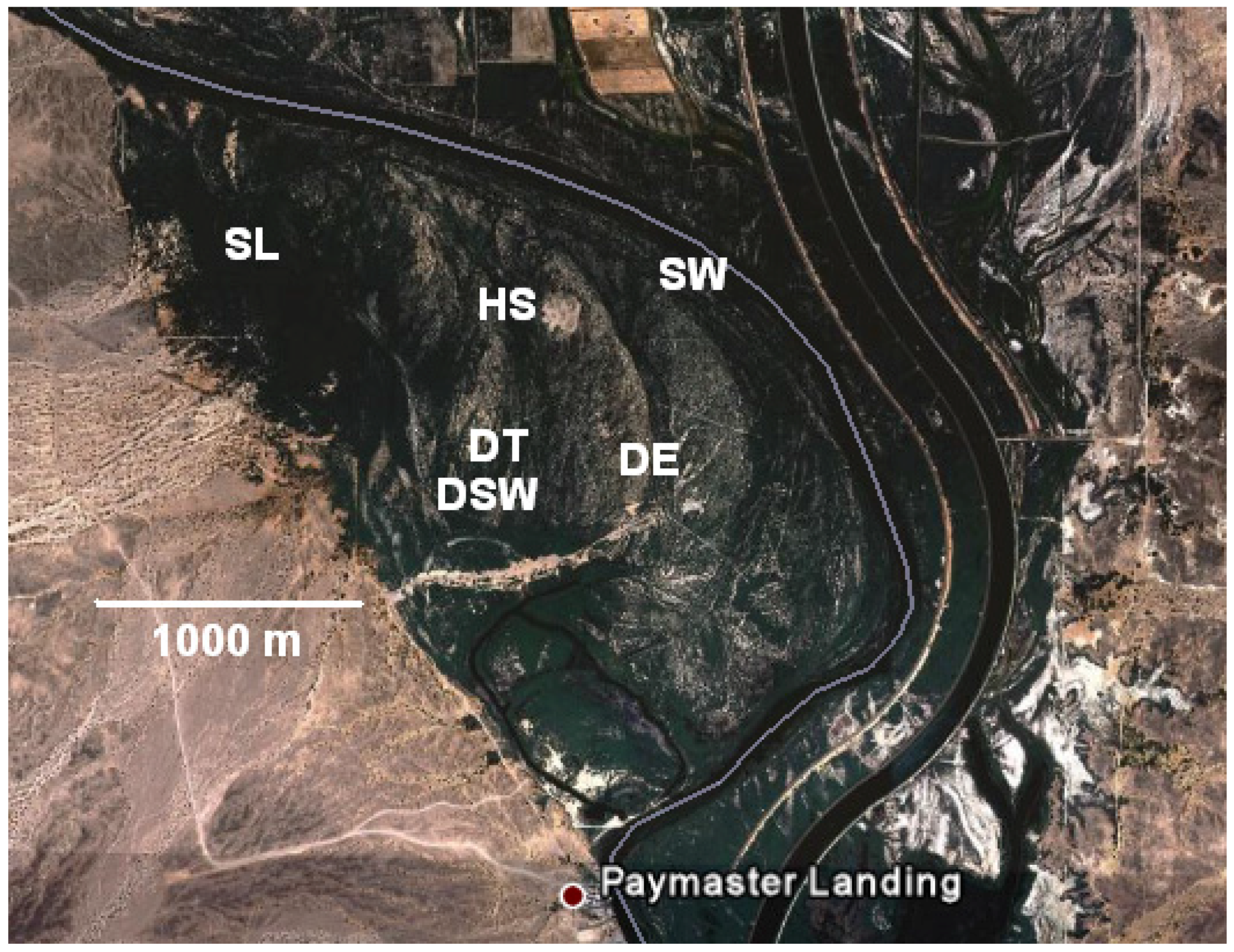
2.1. Site Description

CNWR is located near Blythe, CA, on the Lower Colorado River [8,34]. This is an extreme, low-desert environment. Annual rainfall is under 100 mm yr−1, occurring as occasional winter rains augmented by summer monsoon rains in July and August [35]. The hottest month of the year is August with an average maximum daily temperature of 38 °C and the coolest month is December with an average minimum daily temperature of 4 °C.
Names and locations of measurement sites and soil and aquifer conditions are in Table 1. Sites were given fanciful names based mainly on summer working conditions. Saltcedar study sites were on a floodplain terrace in six plots established at different distances from the active channel of the river (Figure 1). These plots were established by the US Bureau of Reclamation and a consortium of universities with the purpose of developing ETactual estimation methods for western US rivers [7,34]. Three of the sites were equipped with Bowen ratio flux towers but data from the towers are not yet available for comparison with sap flow results. Sap flow measurements for Swamp, Slitherin and Diablo East were reported in Nagler et al. [8] and Hot Springs, Diablo Tower, and Diablo Southwest are reported here. Each plot contained one to five observation wells to measure depth and salinity of the aquifer. The Hot Springs site was on the edge of a bare area in which geothermal water approached within 2.5 m of the surface. Saltcedar was the dominant plant at each site, growing in dense stands interrupted by areas of light, sandy soil, with occasional arrowweed (Pluchia sericea) and quailbush (Atriplex lentiformis) shrubs and stunted screwbean mesquite (Prosopis pubescens) trees occurring in the more open areas. Methods for determining soil and aquifer properties, summarized in Table 1, are described in Nagler et al. [8,34]. Depth to the aquifer and salinity of the aquifer were measured at monthly intervals from 2007–2008. Soil properties were determined at 0.3 m intervals in auger holes bored from the surface to the top of the aquifer at each site in 2008 as described in [34]. Alfalfa ETactual was measured in a well-managed field (Hayday Farms, Inc., Blythe, CA) within the floodplain of the river, approximately 8.4 km from the active channel, in the Palo Verde Irrigation District adjacent to CNWR. The field was 375 m by 815 m (30.1 ha) in area. Bowen ratio and eddy covariance moisture flux towers were installed in the middle of the field, as part of the Bureau of Reclamation ETactual monitoring program. The field was flood-irrigated at ca. 10 day intervals and cut each 30 days in summer, but less frequently in winter.
Table 1. ETactual measurement sites for saltcedar and alfalfa on the Lower Colorado River. ETactual for alfalfa and for saltcedar at Diablo SW, Diablo, and Hot Springs were measured in the present study. Data for Swamp, Slitherin and Diablo East were from [7]. Soil texture data are % sand (S), silt (Si) and clay (C). Numbers in parentheses are standard errors of means.
SiteLat/Lon (o North, o West)Distance From River (m)Soil Texture (S-Si-Cl)Depth to Aquifer (m)Aquifer Salinity (dS m−1)Aquifer Temperature (oC)
Swamp33.2754,
114.6873
20025-55-202.35 (0.03)3.90 (0.18)23.1 (0.3)
Slitherin33.2746,
114.7098
75040-45-153.51 (0.06)4.72 (0.48)22.5 (0.2)
Diablo Tower33.2659,
114.6992
150050-35-152.61 (0.06)15.49 (0.18)22.8 (0.3)
Diablo Southwest33.2663,
114.7002
155090-7-32.79 (0.06)24.0 (0.55)22.2 (0.2)
Diablo East33.2687,
114.6895
87095-2-32.40 (0.04)7.1 (0.19)24.9 (0.2)
Hot Springs33.2783,
114.6924
55785-10-52.36 (0.03)5.39 (0.07)51.0 (0.5)
Hayday Farms Alfalfa33.4683,
114.6938
8,439-1.81 (0.05)1.85 (0.05)23.0 (0.35)
Figure 1. Sap flow measurement sites for saltcedar at Cibola National Wildlife Refuge. SL = Slitherin; HS = Hot Springs; SW = Swamp; DT = Diablo Tower; DSW = Diablo Southwest; DE = Diablo East.
Remotesensing 01 01273 g001

2.2. Sap Flow Measurements

Sap flow was measured by the tissue-heat-balance method as described in Sala et al. [31], Grime and Sinclair [36], Kjelgaard et al. [37] and Nagler et al. [8,38,39]. We used home-made sensors described in Scott et al. [40], which were field-validated by measurements of ETactual by flux towers [40]. In the tissue-heat-balance method, an intact branch containing leaves is wrapped by a heating wire and a constant source of low-grade heat is applied to the branch. Thermocouples embedded in the branch measure temperatures upstream and downstream from the heat source, and a thermopile outside the heating wire in the surrounding layer of insulation measures heat lost radially from the branch. A heat balance equation is then solved to calculate heat transported by convection in the transpiration stream, and the results are expressed in terms of grams of water transported per hour. Diurnal patterns of transpiration were combined with diurnal patterns of atmospheric water demand as measured by vapor pressure deficit (D) to calculate stomatal (canopy) conductance (GS) [41,42].
Branches ranged from 5 mm to 15 mm in diameter. The sensors and thermopile were wrapped in insulating foam and covered with reflective foil to minimize solar heating. An instrument station containing a solar panel, four 6 volt batteries, one to three multiplexers, a voltage regulator, and a data-logger was established in each plot. A computer program transformed temperature data from the sensors into sap flow rate per hour. This program also filtered the data to remove aberrant values. The sensor readings were processed with a Matlab (MathWorks, Inc., Natick, MA) script composed by us.
In 2007, saltcedar transpiration was measured on eight plants at Slitherin from July 20-September 2; five plants at Diablo East from June 22-July 8; and seven plants at Swamp from June 20-July 17 (reported in [8]). In 2008, saltcedar transpiration was measured on eight plants at Diablo Tower from August 8-August 16; 11 plants at Diablo Southwest from July 3-July 18; and 10 plants at Hot Springs. At the end of each measurement period, gauged branches were harvested and brought to the Environmental Research Laboratory in Tucson, Arizona, for determination of leaf dry weight and leaf area per branch.
Calculation of sap flux requires a correction for conductive heat loss that occurs in the absence of sap flux, which is usually accomplished by assuming that sap flux goes to zero between 2–4 am each day, and using temperature readings during those hours as zero points. However, saltcedar is now known to transpire at night [8,43]. Therefore, at the end of each sap flux measurement period, we continued to measure temperatures for two hours after harvesting the branch above the point where the sensor was attached, and those temperature values were used as zero points for calibrating sensors.

2.3. Scaling ETactual to Whole Plants and Stands of Plants Based on Leaf Area Index

Sap flow data were collected in units of grams of water transported per hour through a gauged branch. Data were converted to volume of water loss per m2 of leaf area (EL), canopy area (EC) or ground area (EG) per day, expressed as mm d–1 of water loss over an indeterminate surface area. For comparison with stomatal conductance over diurnal cycles, EL was also expressed as mmol H2O m−2 sec−1 [41,42].
To convert E to EL, grams dry weight of leaves for each branch were converted to m2 of leaf area by determining Specific Leaf Area (SLA) (m2 one-sided leaf area per g dry weight of leaves) for fresh leaf samples from 10 different plants per site. Surface area was measured by placing fresh leaves flat side down on a sheet of graph paper, then counting the number of grid intersections covered by leaves (the point intercept method). The area per grid multiplied by number of grid intersections covered gave the area covered by leaves. Then the leaves were dried in an oven (60 oC) to determine dry weight, and SLA per branch was used to calculate EL. SLA for saltcedar was 0.0079 m2 g−1 (SE = 0.0004). Methods are described in more detail in Nagler et al. [44].
To convert EL to EC, plant-specific leaf area index (LAPS) was measured within plant canopies over the plot area:
EC = EL × LAPS
To covert EL to EG, LAI on a ground-area basis was calculated as:
LAI = LAPS × fc
where fc is fractional vegetation cover and:
EG = LAI × EL
We used a Licor LAI 2000 meter (Licor Inc., Lincoln, NE) to measure LAPS at 50–100 points within each plant stand, collecting readings in June, July and August, 2007 and 2008. We calibrated the Licor LAI 2000 readings against leaf harvest methods by recording LAPS by Licor LAI 2000 under selected canopies for which we also harvested leaves to determine LAPS [8]. We placed a 0.25 m2 PVC plastic frame horizontally over the canopy at the point where LAPS was measured by Licor, then harvested all the leaves within the frame. The leaves from these quadrant samples were then dried and weighed, allowing us to express the sap flow results in terms of water loss per m2 of canopy area, by making a ratio between the g leaves per sap flow branch and the g leaves per m2 of canopy determined by the quadrant harvests. LAPS values measured by Licor LAI 2000 were multiplied by 0.84 to make them consistent with leaf-harvest LAPS values.
To calculate fc, we used high resolution (1 m) aerial photographs collected by Chris Neale (Utah State University) in June, 2007. We measured fc over an area of approximately 6 ha around each site, in order to extrapolate EG to the footprint size of MODIS pixels, used to scale EG over the floodplain. Each image was imported into a viewing program (Adobe Photoshop) and a grid (ca. 200 squares) was placed over the image. Each grid intersection was visually scored as either bare soil or vegetation (visible as false-color red from the NIR band in the photos). Visual scoring was used instead of a spectral classification method due to the presence of shadows, which interfered with spectral methods [34]. Since saltcedar made up > 90% of the vegetation at each site, EG was based only on saltcedar transpiration rates.

2.4. Measurement of Alfalfa ETactual

Alfalfa ETactual was measured by soil moisture depletion using a neutron hydroprobe (503 DR Hydroprobe, Campbell Pacific Nuclear, Inc., Concord, CA) following methods in Bell [45] and Glenn et al. [46]. In 2006, five PVC (Schedule 40) neutron hydroprobe access tubes were installed 100 m from each of the four corners and in the center of the alfalfa field. The neutron hydroprobe was calibrated to convert counts per minute (cpm) to volumetric moisture content (cm3 H2O cm−3 soil). We determined bulk density by extracting soil cores near each hydroprobe port with a volumetric soil-sampling auger. We then measured cpm at the 60 cm depth at each hydroprobe port. Soil moisture was determined in the laboratory on soil samples taken at each probe port at the same time and soil depth as neutron hydroprobe readings. Bulk density of the soil was 1.50 g cm−3. The linear equation relating soil moisture to cpm was:
Soil Moisture (cm3 H2O cm−3 soil) = 0.0000467 cpm − 0.0246 (r2 = 0.998)
ETactual was estimated in August and September, 2006, and June, 2007, by measuring soil moisture content 48 hours after irrigation and then 6–7 days later at each probe port. The 48-hour delay in taking the initial reading allowed time for water to infiltrate into the soil profile, and for a soil crust to form to reduce surface evaporation. Soil moisture was measured at 0.3 m intervals from the 0.3 m soil depth to 1.8 m depth in the probe ports. The water table was encountered at about 1.8–2.0 m depth.

2.5. MODIS Data

MODIS data from the Terra satellite are collected on a near-daily basis and are processed and composited into 16-day values by NASA’s EROS Data Center, using 3–5 cloud-free images for each collection interval [47]. Both the Normalized Difference Vegetation Index (NDVI) and the Enhanced Vegetation Index (EVI) are available as georectified and atmospherically corrected products with a resolution of 250 m. We used EVI instead of the more commonly used NDVI because previous studies [17] showed that ETactual measured at 11 moisture flux tower sites was significantly better correlated with MODIS EVI than NDVI (see also [9]). EVI is calculated as:
EVI = 2.5 × (ρNIR − ρRed)/(1+ ρNIR + (6 × ρRed − 7.5 × ρBlue))
where the coefficient "1" accounts for canopy background scattering and the blue and red coefficients, 6 and 7.5, minimize residual aerosol variations. We converted EVI to a full scale between 0 and 1 (EVI*):
EVI* = 1 − (EVImax − EVI)/(EVImax − EVImin)
where EVImax is the value for full plant cover and EVImin is the value for bare soil. We used values of 0.542 and 0.091, respectively, from a large data set collected over three western riparian zones in a previous study [7]. We used a scaled value of EVI following the recommendation of Choudhury et al. [18], but they noted that regression equations can also be developed using unscaled vegetation indices. Also, our value for maximum EVI was based on riparian canopies in a previous study [7] and alfalfa had EVI* values greater than 1.0 (EVI was not scaled separately for each vegetation type).
MODIS EVI data were obtained from the Oak Ridge National Laboratory DAAC site [47]. This site allows the user to view the footprint of a MODIS pixel or set of pixels displayed on a current, high-resolution Google Earth image before a final selection is made. We used this feature of the ORNL DAAC site to ensure that pixels encompassed our areas of interest (e.g., sap flow sites and the alfalfa field), and were not contaminated by adjacent land cover types. For the sap flow sites, a single pixel centered around each site was selected. For the alfalfa field, three adjacent pixels, each wholly contained within the field, were selected. The 16-day period or periods encompassing the dates of ground ETactual collection were obtained.

2.6. Meteorological Data and Other Calculations

Meteorological data for CNWR and the Hayday Farms alfalfa field were obtained from the Parker, Arizona, AZMET station [35]. Data for saltcedar and arrowweed at Havasu National Wildlife Refuge (HNWR) were from the Mojave #2 AZMET station [35]. Two formulations of ETo were used to calculate EToF by Equation (2). The first was the FAO-56 formula for reference crop ETo using the Penman Monteith equation (ETo-PM) (see [19,48] for a description of the meteorological variables, instrumentation and calculation procedures). This is generally the preferred formula for ETo since it includes all the major variables affecting ETactual. However, since it is formulated for a short grass-reference crop under light winds, it is dominated by the radiation term in the Penman Monteith equation, which might not be applicable to riparian vegetation [16]. The Blaney Criddle formulation of ETo (ETo-BC) is based on mean monthly temperature and mean daily percentage of annual daytime hours [49], and over the range of latitudes in the present study it is dominated by temperature, which affects D and is the advective term in the Penman Monteith equation [48]. A previous study [50] found a much better correlation between flux tower ETactual and ETo-BC than ETo-PM. Also, temperature data is much more widely available than the full set of meteorological data needed to calculate ETo-PM. In Arizona, for example, there are nearly 500 cooperative NOAA stations reporting temperature and precipitation throughout the state, but only 27 AZMET reporting ETo-PM. We calculated ETo-BC by the formula in Brouwer and Heibloem [49] using AZMET mean monthly temperature:
ETo-BC = p × (0.46Tmean + 8)
where p is mean daily percentage of annual daytime hours (from a table in Brouwer and Heibloem [49], Tmean is mean monthly temperature in oC, and ETo-BC is in units of mm d−1.
Canopy conductance (GS) on a leaf-area basis (mmol m−2 s−1) was calculated by the formula [41,42]:
GS = EL/D × KG (10)
where KG is the stomatal or canopy conductance coefficient (kPa), calculated from atmospheric pressure corrected for temperature effects by the formula:
KG = 115.8 + 0.4226T
The term EL/D × KG is the ratio of transpiration to atmospheric water demand, and it is related to the degree of stomatal opening at a given time of day [48].
For unstressed crops, diurnal patterns of EL closely follow the net radiation (Rn) curve, and the evaporative fraction (EF) is generally constant during the daylight hours [6,51,52]:
EF = λEG/Rn
where λEG is the latent heat of evaporation (W m-2) calculated from hourly values of EG measured by sap flow sensors, assuming a heat of evaporation of 2,257 kJ kg−1 water [48]. Hourly values of Rn were calculated as 0.77 Rs measured at the Parker AZMET station, assuming an albedo of 0.23 [19]. Equation 12 is used to scale instantaneous estimates of ETactual, made using thermal bands on satellites at midday, to daily time steps [6,52]. Diurnal plots of EF can also be used to diagnose stress effects on photosynthesis and stomatal conductance [53,54]. Estimates of saltcedar EG from EL, LAPS and fc in Equation 5 are susceptible to propagation errors due to separate errors in estimating each term in the equation [55]. The propagation error was calculated based on the standard error the mean of each variable using software in [56].

2.7. Other Sources of EG and ETactual Data

In addition to the data collected here, the final ETactual algorithm based on Equations 1 and 2 contained additional published data collected for riparian plants on the Lower Colorado River. Two years of saltcedar data and one year of arrowweed data were collected at HNWR, in which ETactual was measured by Bowen Ratio moisture flux towers [7,30]. One year of EG data were collected by sap flow sensors for cottonwood at CNWR in 2005 [38]. One year of EG and GS data were collected by sap flow sensors at three different saltcedar sites than those in the present study at CNWR in 2007 [8]. For these sites, summer ETactual or EG values were matched with single MODIS pixels encompassing each site, and EVI* and EToF over each measurement period were calculated.

3. Results

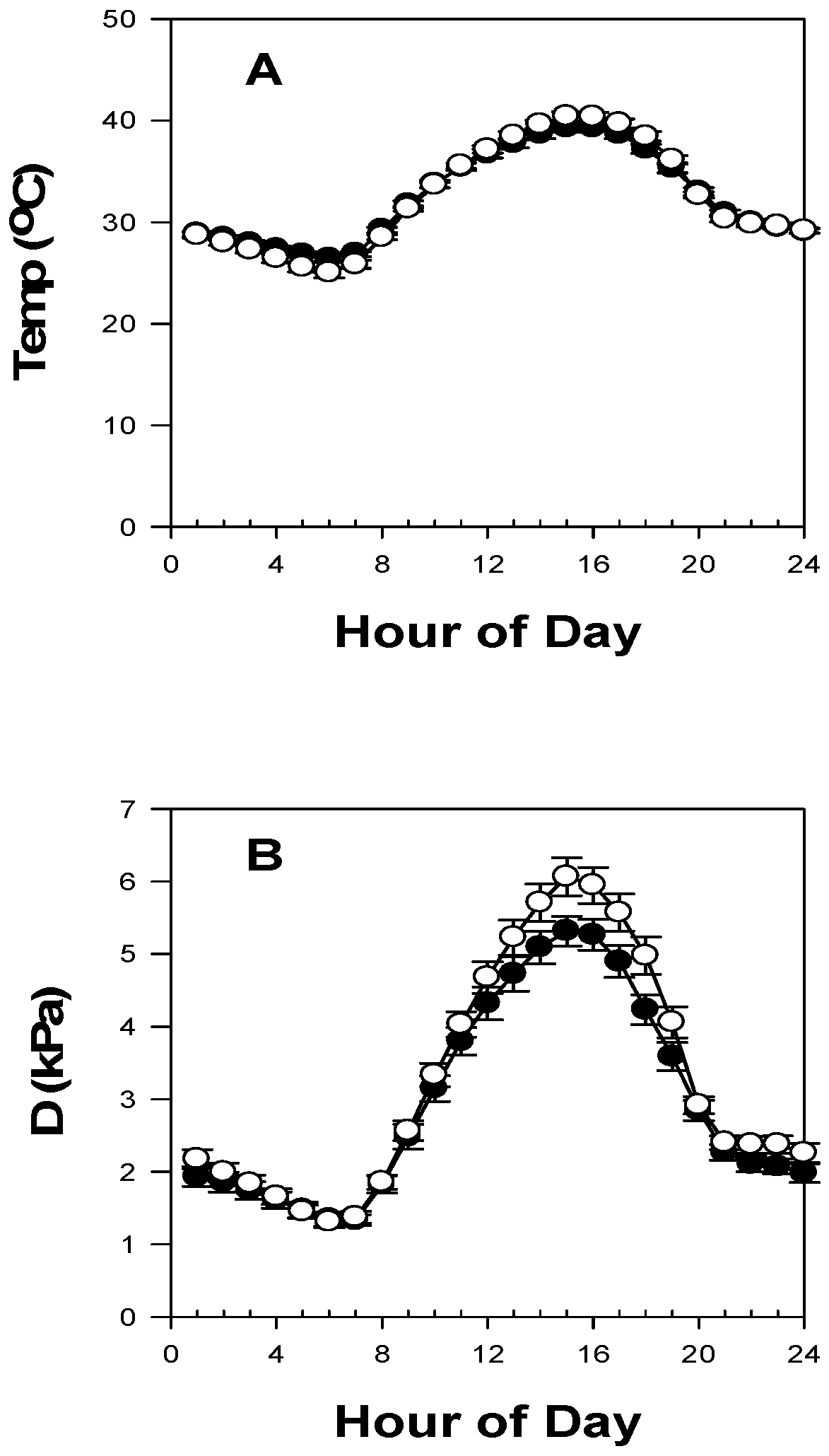
3.1. Meteorological, Soil and Aquifer Conditions at Saltcedar and Alfalfa Sites

Diurnal temperature, vapor pressure deficit, and radiation curves from the Parker AZMET station over the 2007 and 2008 sap flow measurement periods (June-August), are in Figure 2.
Figure 2. Climate conditions measured at the Parker, Arizona, AZMET station during periods in which sap flow measurements were made at Cibola National Wildlife Refuge in 2007 (closed circles) and 2008 (open circles). Values are means over the June-August measurement intervals of air temperature (A), vapor pressure deficit (B), and solar radiation (RS) (C).
Remotesensing 01 01273 g002aRemotesensing 01 01273 g002b
Conditions were similar both years, characterized by bright, hot days with very high midday atmospheric water demand. Rainfall over the measurement periods was 2.0 mm in 2007 and 8.8 mm in 2008. Sites differed in soil properties, depth to water, and salinity of the aquifer (Table 1). Soils at Swamp and Slitherin were loams, whereas soils at Diablo Tower, Diablo Southwest, Diablo East and Hot Springs were sands. The water table was deeper at Slitherin (3.5 m) than at the other saltcedar sites (2.4–2.8 m). Aquifer salinities ranged from 3.90 dS m−1 at Swamp to 24.0 dS m−1 at Dialbo Southwest and salinity increased in direct proportion to distance from the active channel (r2 = 0.82. P = 0.005). The equation of best fit was:
EC (dS m−1) = 0.012 d − 0.626
where EC is electrical conductivity and d is distance from the river in meters. A value of 1.41 dS m−1 for river water was used as the zero distance value. Aquifer temperatures were markedly elevated at Hot Springs due to the intrusion of geothermal water into the aquifer. The alfalfa field had a clay loam soil, and an elevated, non-saline aquifer due to the effect of irrigation.

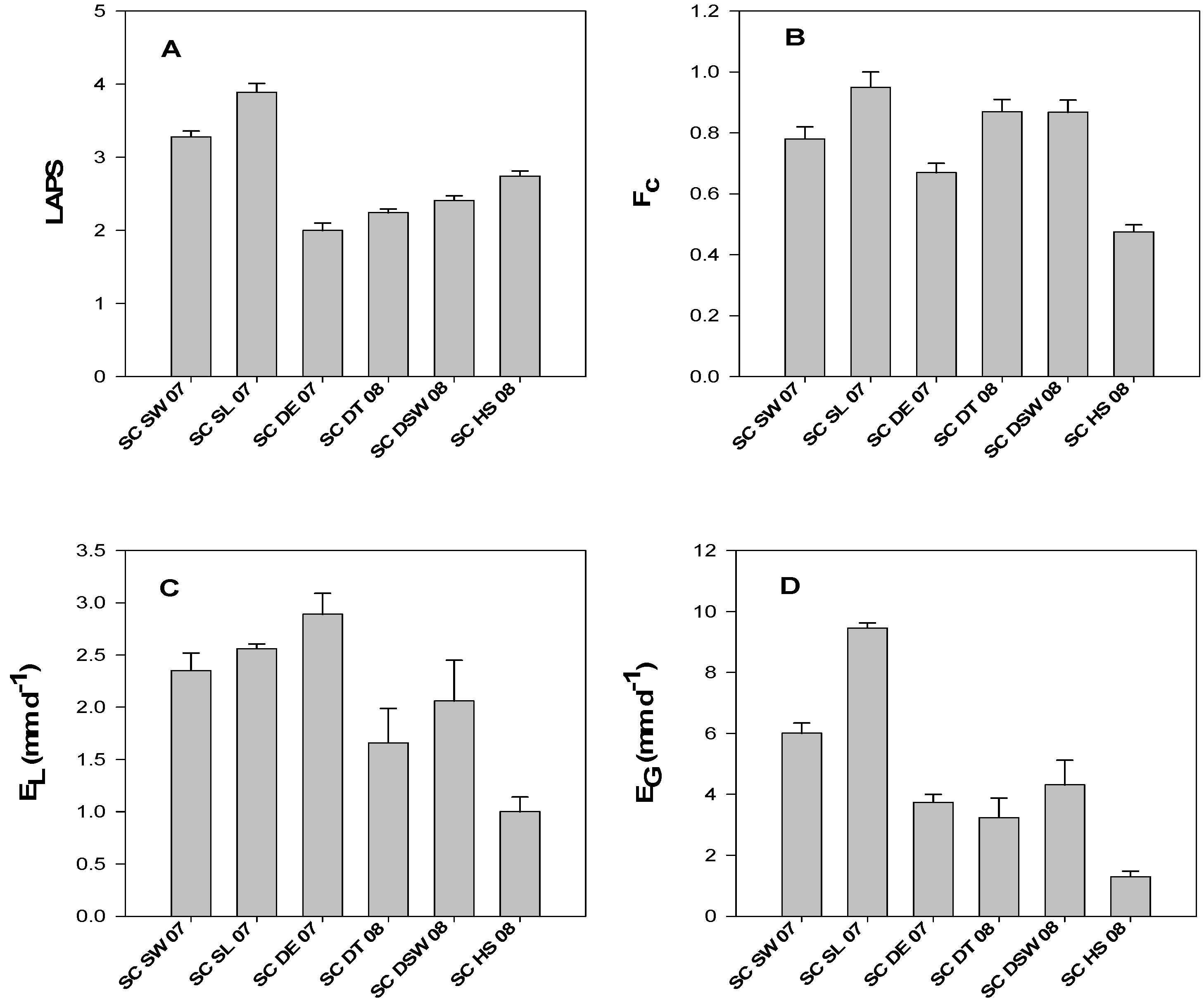
3.2. LAPS, fc, EL, and EG of Saltcedar Stands

LAPS varied from 2–4 among saltcedar sites (Figure 3A) but did not vary significantly (P > 0.05) from June to August at a given site [8]. fc varied from 0.47–0.95 (Figure 3B). EL (Figure 3C) and EG (Figure 3D) was markedly lower at Hot Springs than at other sites. We attribute this to the elevated aquifer temperatures. Excluding Hot Springs, mean EL was 2.30 mm d−1 and the coefficient of variation (CV) was 0.20; mean EG was 5.35 mm d−1 and CV was 0.47. Over all sites, standard errors of EL, LAPS and fc were 4.7%, 2.1% and 0.7% of mean values, respectively, and the cumulative propagation error for EG was 6.5% of the mean value across sites.

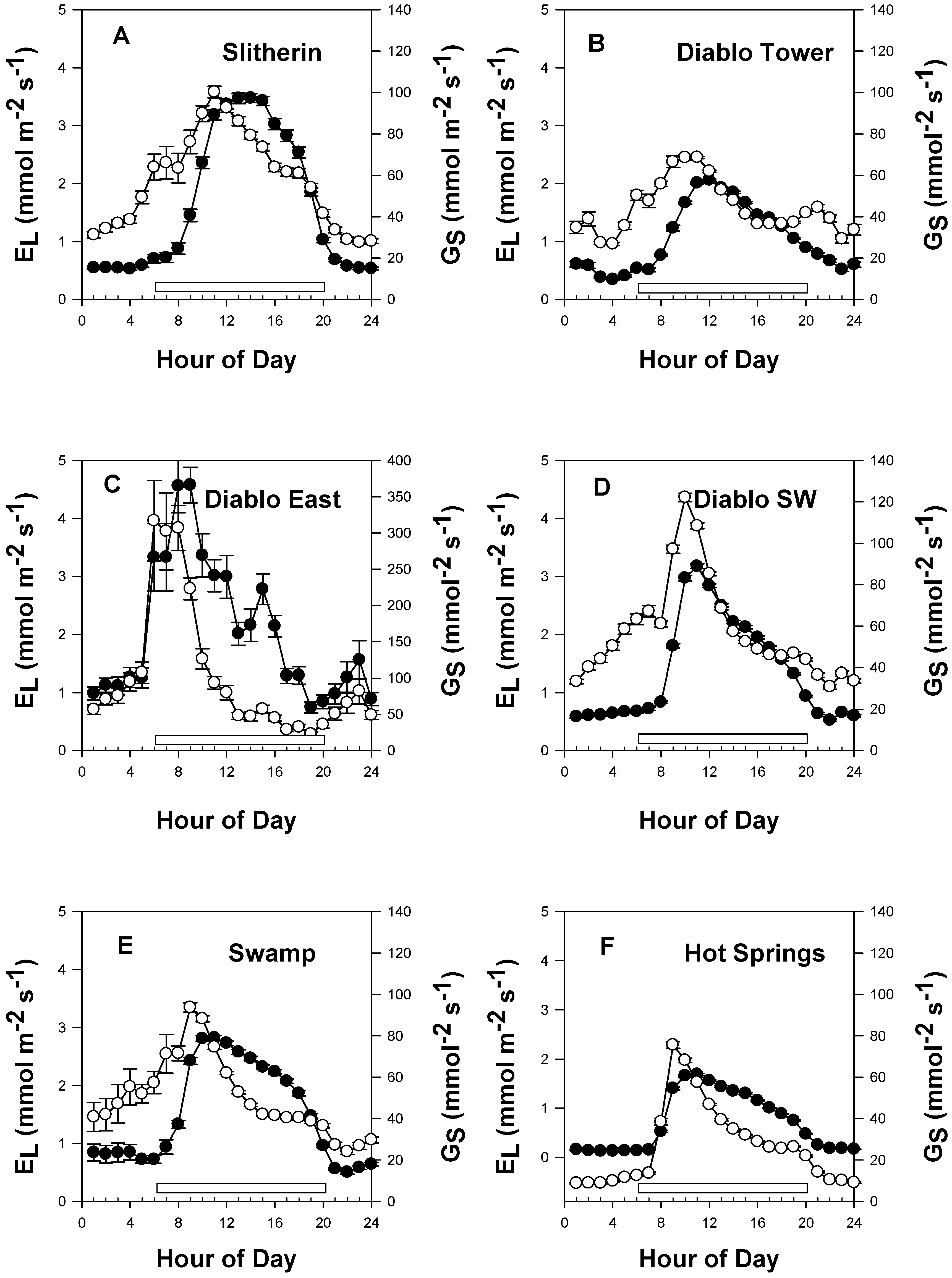
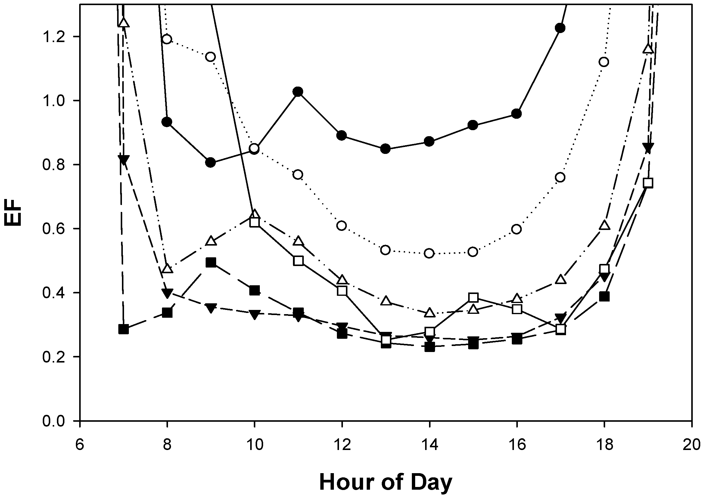
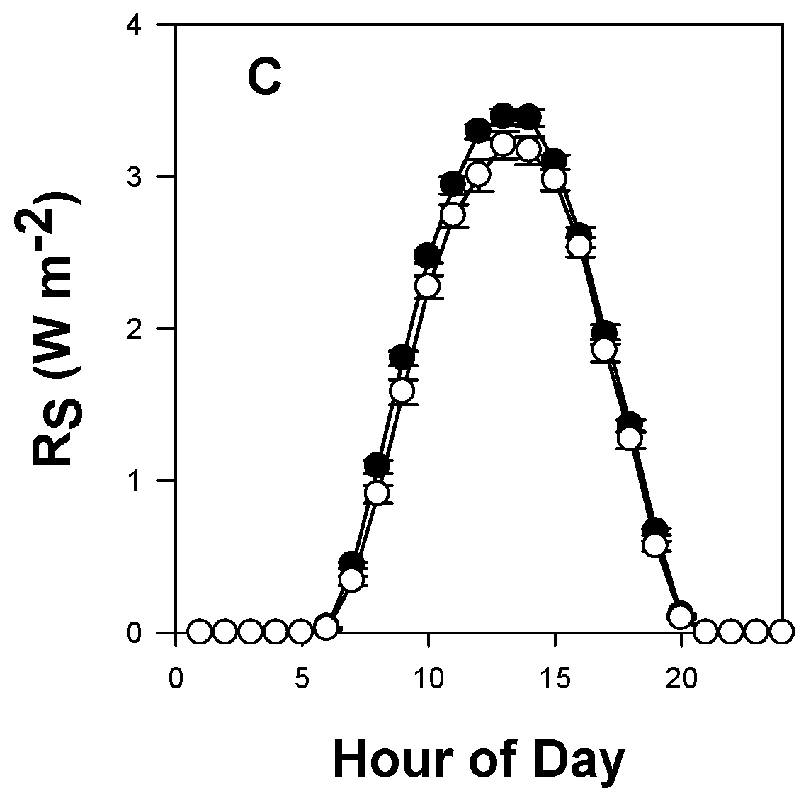
3.3. Diurnal Variation in EL, GS and EF

Saltcedar showed markedly different patterns of EL and GS among sites (Figure 4). Slitherin (Figure 4A) was the only site where EL closely tracked the daily radiation curve (r2 = 0.92, P < 0.001), with peak EL at 1,200–1,300 hrs, and peak GS at 1,000 hrs. The other sites had peak EL well before 1,200, and afternoon EL was truncated when compared to the radiation curve. Diablo East had peak EL at 0800 hrs and peak GS was at sunrise (0600 hrs) then dropped after 0800 hrs. All sites tended to show a recovery in GS between 1,600 and sunset. All plants also continued EL at night, with nocturnal water loss accounting for 25% of total EL across sites. The foliage of the plants was heavily coated with highly saline water droplets at dawn, even though temperatures were well above the dew point, indicating that much of the nighttime water loss could be due to guttation through salt glands on saltcedar leaves [57] rather than transpiration through stomata.
Diurnal curves of EF showed U shapes typical of crops, for which EF often exceeds 1.0 in early morning and late afternoon, when advective effects dominate ETactual, but are less than 1.0 during midday hours, when ETactual is limited by Rn, which supplies the energy needed to evaporate water [6,48,51,52]. However, patterns of saltcedar EF were not constant over the daylight hours at most of the sites (Figure 5). Morning values of EF (i.e., 0800–1200 hrs) were 0.53 (SE = 0.065), compared to only 0.35 (SE = 0.019) in the afternoon (1,300–1,700 hrs) due to the midday depression of EL and GS across sites. Slitherin was the only site for which midday EF was in the range of 0.8–1.0, indicating the maximum utilization of available energy to support EG, while the other sites ranged from 0.3–0.5.
Figure 3. Saltcedar plant-specific leaf area index (LAPS) (A), fractional cover (B), leaf-area transpiration (C) and ground-area transpiration (D) at six sites at Cilobla National Wildlife Refuge on the Lower Colorado River.
Remotesensing 01 01273 g003
Figure 4. Leaf-area transpiration (EL) (closed circles) and stomatal conductance (GS) (open circles) of saltcedar at six sites at Cibola National Wildlife Refuge on the Lower Colorado River. Results are hourly mean values over each measurement period. Error bars are standard errors. Horizontal white rectangles above the x-axis denotes daylight hours.
Remotesensing 01 01273 g004
Figure 5. Evaporative fraction (EF), defined as ETactual/Rn, for saltcedar at six sites at Cibola National Wildlife Refuge on the Lower Colorado River. Sites are Slitherin (closed circles), Swamp (open circles), Diablo Tower (closed triangles), Diablo Southwest (open triangles), Hot Springs (closed squares) and Diablo East (open squares).
Remotesensing 01 01273 g005

3.4. Alfalfa ETactual

ETactual measurements were made when plants were 30–50 cm tall and had not been recently cut. LAI measured by Licor LAI 2000 during the June, 2007 measurement period was 4.42 (Std. Error = 0.42). Soil moisture depletion in units of cm3 cm−3 d−1 were converted to ET units (mm H2O d−1) based on water loss in the top 1.8 m of soil profile. ETactual in the alfalfa field ranged from 6.96 mm d−1 at the end of September, 2006, to 8.77 m d−1 in early June, 2007 (Figure 6). The standard error of mean ETactual tended to be high at each sample date, due to variation in ETactual among the five sites within the field. However, differences in soil moisture content at the two sampling dates in each measurement period were significant across soil depths and probe ports for all measurement periods (P < 0.05).
Figure 6. Alfalfa ETactual at a field in the Palo Verde Irrigation District calculated from the difference in soil moisture levels measured 48 hours after an irrigation (closed circles) and 6–7 days latter (open circles). Each data point is the mean of five probe measurements. SE is the standard error of ETactual over all five ports. P is the probability that mean moisture contents across soil depths are equal at the two measurement intervals by paired t-test.
Remotesensing 01 01273 g006aRemotesensing 01 01273 g006b

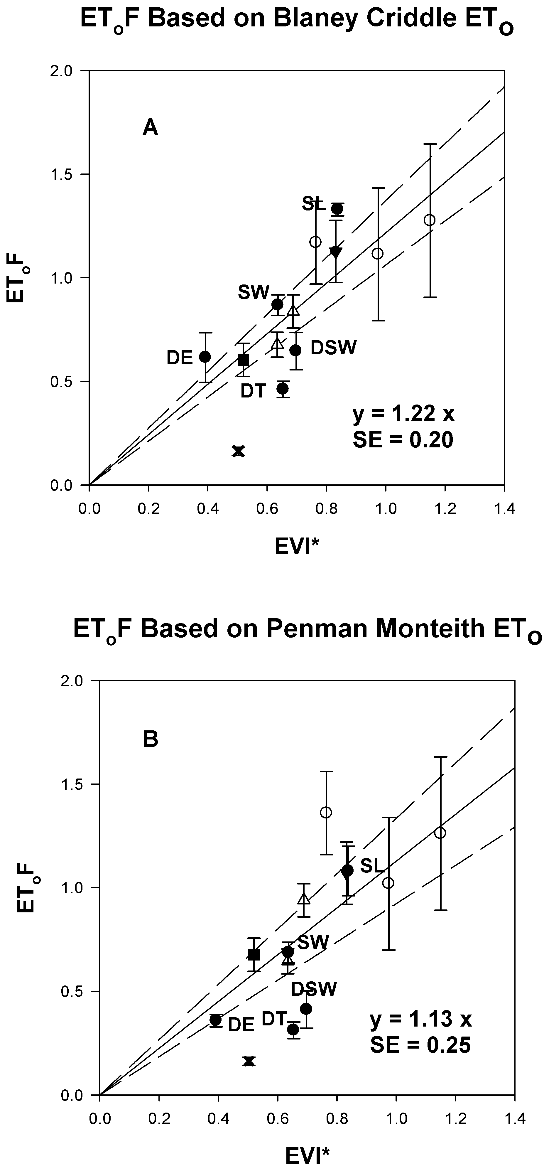
3.5. Linear Equations for EGF and EToF Based on EVI*

For the eight saltcedar data points (six sites at CNWR and two years data at one site at HNWR), the correlation between EG or ETactual and EVI* was significant (P = 0.036) but of low predictive power (r2 = 0.55). We attempted to improve and generalize the algorithm by normalizing EG data to reference crop ETo, and by including other plant types. Hot Springs was not included in the regression equations as it was clearly an outlier due to the elevated aquifer temperatures. Linear regression equations between EToF and EVI* were significant for both ETo-BC and ETo-PM (P < 0.01), but y-intercepts were small and non-significant (P = 0.69 and 0.84, respectively). This is expected because the scaling procedure sets EVI* for bare soil at 0. Therefore, it was justified to pass regression equations through the origin to determine the final algorithms (Figure 7). ETo-BC (Figure 7A) clearly gave a better fit of data than ETo-PM (Figure 7B). The standard error of the mean increased with increasing EToF, as expected for regression through the origin. At EToF = 1.0, the error around the mean for the expression using ETo-BC was about 20%, compared to 25% for ETo-PM. When only saltcedar EToF was used in the regression with EVI*, the slope of the EToF:EVI* equation based on ETo-BC was 1.20, nearly the same as when all plants were included (1.22) (no significant difference in slopes at P = 0.05), hence the equation in Figure 7A can be used to estimate EToF for either saltcedar or mixed stands of agricultural and riparian plants on the Lower Colorado River.
Figure 7. Ratio of ETactual or EG to reference crop ET (EToF) for plants on the Lower Colorado River, using the Blaney Criddle method (A) and the Penman Monteith method (B) for ETo. Plants and locations are: saltcedar at Slitherin (SL), Swamp (SW), Diablo East (DE), Diablo Southwest (DSW) and Diablo Tower (DT) at Cibola National Wildlife Refuge (closed circles); saltcedar at Hot Springs at Cibola National Wildlife Refuge (cross); saltcedar at Havasu National Wildlife Refuge in 2002 and 2003 (open triangles); arrowweed at Havasu National Wildlife Refuge in 2003 (closed square); and alfalfa at Palo Verde Irrigation District on three dates (open circles). Hot Springs was not included in the regression analyses. Regression equations were passed through the origin and dashed lines denote 95% confidence intervals. Error bars are standard errors of means.
Remotesensing 01 01273 g007
The reason for the better performance of ETo-BC compared to ETo-PM was further investigated with flux tower data for saltcedar at HNWR (from data in [7]). Over an annual cycle, ETo-BC was about 10% lower than ETo-PM and they had slightly different seasonal curves, with the temperature-driven ETo-BC lagging behind the radiation-driven ETo-PM in the spring (Figure 8). Saltcedar loses its leaves in winter and does not green up until mid-March, and when flux tower data for saltcedar ETactual was plotted against ETo, its phenology better matched ETo-BC than ETo-PM (Figure 8).
Figure 8. ETo calculated by the Penman Monteith method (ETo-PM), the Blaney Criddle method (ETo-BC) and saltcedar ETactual measured by Bowen ratio moisture flux towers at Havasu National Wildlife Refuge on the Lower Colorado River in 2002 and 2003. Data are from [7]. Correlation coefficients (r) between each variable are shown under the curves.
Remotesensing 01 01273 g008

4. Discussion

4.1. Diurnal Patterns of Saltcedar EL, GS and EF Indicate Stress

The study site at CNWR was selected as typical of the dense saltcedar stands that have developed on wide river terraces on the Lower Colorado River. Due to lack of overbank flooding, the aquifer has become salinized, and it is dominated by saltcedar and native salt tolerant shrubs. The aquifer is replenished by underflow from the river, and the salinity of the aquifer increases in proportion to distance from the river, due to extraction of water by saltcedar while most of the salts remain in the aquifer [8,34].
Except at Slitherin, diurnal patterns of EL and GS were not at all typical of unstressed crop plants. At the other sites, saltcedar exhibited marked midday depression of EL and GS, a characteristic of stressed plants [21]. Furthermore, the response was not uniform among sites; in fact, saltcedar at each site exhibited different diurnal patterns of E, GS and EF. Peak EL at Slitherin was at 1,200 hrs, whereas plants at Diablo East had peak EL at 0800 hours and the other sites were intermediate. Other studies have also noted midday depression of saltcedar ETactual [31,58,59,60].
Saltcedar at Hot Springs was obviously affected by high temperatures in the aquifer. However, the factors controlling EL and EG at the other sites were not as clearcut. Depth to the aquifer did not seem to be a controlling factor, since the aquifer was deepest at Slitherin, which had the highest values of LAPS, fc and EG. High salinity might have negatively affected plants at Diablo and Diablo SW, but Slitherin outperformed plants at Swamp, Diablo East and Hot Springs, despite having similar salinities as those sites.
Soil conditions in the aquifer differed among sites and could be responsible for differences in diurnal responses. EL and EG of phreatophytes can be profoundly affected by soil texture, which regulates the rate at which roots can extract water from the aquifer [61]. Sands (as at Hot Springs, Diablo Tower, Diablo Southwest and Diablo East) have low matric potential, and water in the rhizosphere can cavitate above a critical level of EL, limiting transpiration rates in sandy aquifers [62]. On the other hand, heavier soils as at Slitherin can support higher rates of EL due to less tendency for the water column to cavitate at the soil-root interface [62]. A working hypothesis, which we have not yet tested, is that the soil in the root zone of saltcedar recharges with water at night, but is depleted faster than it can be replenished in the morning, leading to midday depression of saltcedar EL at the sites with sandy soils. This could lead to the observed patterns in which morning EF was much higher than afternoon EF at all sites except Slitherin. In support of this hypothesis, EG was negatively correlated with % sand (r = −0.612) and positively correlated with % clay (r = 0.543) (P > 0.05, not significant, for each), and a multiple linear regression between EG and % sand and % clay had r = 0.91 (significant at P = 0.029), despite the small sample size (6 sites).
Unlike most crop plants [63], saltcedar has high rates of nocturnal water loss, amounting to 25% of total consumptive use in this study and even more in a study on the Middle Rio Grande [43]. Part of this water loss was due to guttation of liquid water rather than EL. Guttation of water through salt glands is functional in disposing of excess salts from the leaf apoplast [57].

4.2. Remote Sensing Algorithm for Scaling ETactual

Given the diverse physiological responses of saltcedar at different sites, caution is needed in using remote sensing methods to scale riparian ETactual over wide areas. With respect to SEB methods, the assumption of constant EF over daylight hours was not met for saltcedar. A midday snapshot of ETactual by satellite would tend to underestimate daily ETactual, and the error would vary from site to site and with the timing of the satellite overpass. With respect to VI methods, EL was not constant on a daily time step, but varied from 1.66–2.89 mm m−2 d−1 among sites (excluding Hot Springs, which was 1.0 mm m−2 d−1). Hence, an ETactual estimate based on the assumption of a constant relationship between EL and ETo (e.g., [1]) would not accurately project ETactual at any given site. In aggregate, however, EToF from saltcedar sites plotted against EVI* fell along the same line as alfalfa, arrowweed and cottonwood. Midday depression of saltcedar EL was compensated by nighttime transpiration and guttation, and a generalized algorithm for scaling ETactual over mixed scenes had an error term of about 20% (mean ETactual = 6.2 mm d−1, SEM = 1.2) when ETo-BC was used for reference ET. This is within the accuracy range of other remote sensing methods for ETactual, which have error rates of 15–30% when compared to ground measurements [14,16]. Hence, the algorithm developed here was within the accuracy range of other methods, and appears to be valid for scaling ETactual over the Lower Colorado River. However, the existence of sites such as Hot Springs, which had aberrant values of EG in relation to EVI*, suggests that the ecophysiological constraints on EG should be characterized by ground studies in a biome of interest, before remote sensing methods are used to scale physiological functions such as EG.

4.3. Comparison with Other Remote Sensing Methods for ET

Nagler et al. [7,50] developed a similar VI method for riparian ETactual, in which time-series flux tower ETactual data were regressed against EVI* from MODIS and meteorological data collected at the flux tower sites. In those studies maximum daily temperature had the most explanatory power among meteorological variables, and addition of other variables did not improve the regression equation. The present results support that study, in that ETo-BC (largely driven by temperature) had more explanatory power than ETo-PM (largely driven by radiation) [16]. Desert agricultural and riparian ETactual rates can be enhanced by advective effects from the surrounding arid landscape, which increases with increasing temperatures (discussed in [16]). Saltcedar ETactual rates projected for CNWR based on methods in [7] are about 20% higher than those projected in this study [34], perhaps due to the use of flux tower data in [7] versus primarily sap flow data in this study. Flux tower data includes both bare soil evaporation and transpiration while sap flow only measures transpiration.
Most remote sensing methods for estimating ETactual have used thermal data from satellite sensors to solve the surface energy balance (SEB) [14,15,64], and several of these have been developed as commercial products [65,66]. Most of these methods require high-resolution thermal imagery (e.g., from Landsat satellites), which have reduced temporal resolution compared to MODIS. Gonzalez-Dugo et al. [6] found similar levels of accuracy of daily ETactual predictions for a VI/crop coefficient method based on FAO-56 [19] and SEB methods based on thermal NIR satellite bands. However, the sources of error were different. SEB methods were affected by the assumption of constant EF, needed to scale instantaneous measurements to daily values, and by differences in calibrating radiometric temperatures to give aerodynamic surface temperatures. On the other hand, the VI method was unable to detect early signs of water stress, whereas SEB methods detect stress as an increase in sensible heat flux at a given value of vegetation cover. Since saltcedar plots in this study exhibited variable degrees of stress, SEB methods could conceivably give a more accurate spatial depiction of ETactual over a floodplain than simple VI methods. Time-series VI methods based on MODIS can provide the primary ETactual data needed in constructing agricultural and riparian water budgets, but these should be augmented by high-resolution SEB methods for detecting stress at the level of individual agricultural fields or stands of riparian plants in western riverine irrigation districts. A combined approach would provide the information needed to monitor consumptive water use and improve water use efficiency of managed and natural vegetation in these districts.

4.4. Sources of Error and Uncertainty

Remote sensing estimates of ETactual are subject to a number of sources of error and uncertainty, as already noted. The main sources of error in this study are outlined below:
A. Several methods were used to measure ETactual on the ground, including sap flow sensors, flux towers, and neutron probe water balance measurements. Each of these havs their own, separate, sources of measurement and scaling errors, and they do not strictly measure the same thing. Sap flow sensors measure plant transpiration while towers and hydroprobe methods measure total ETactual.
B. The sample size and duration of measurements unavoidably varied among plant types. Single alfalfa, cottoonwood and arrowweed sites were measured, whereas six sites were measured for saltcedar. Sap flow sensors measure plant water use over a period of weeks, compared to years for tower measurements. Hence, A and B introduce uncertainty into the ground measurements used to calibrate remote sensing algorithms. These errors are in the range of 10–40% across methods and depend in part on the skill of the practicioners (reviewed in [67]).
C. Vegetation index methods for ETactual cannot account for stress effects, which proved to be substantial and to differ across different plant stands for saltcedar. A strength of the algorithm developed in this study was that it could be applied across different plant types, because even high-resolution satellite imagery cannot resolve the different riparian and agricultural plants present in mixed landscapes on western rivers. However, pooling of crop types inevitably obscures likely difference in transpiration efficiency and other physiological factors that affect leaf-level transpiration rates, thereby introducing additional uncertainty into the remote sensing estimates.
D. The resolution of the imagery and other scaling issues also introduce uncertainty into the estimates. MODIS pixels encompass 6 ha and often contain mixed cover types, but they offer the advantage of high temporal resolution, with near daily coverage. On the other hand, Landsat and other higher resolution images, used in other studies (e.g., [1,6]), leave gaps of weeks or months between measurements.
On balance, the present method offers sufficient accuracy to improve our estimates of ETactual over the range of crops and climatic conditions for which it was calibrated, but does not provide a general algorithm for ETactual for other applications. Fortunately, there are now hundreds of ground stations collecting ETactual data in different biome types around the world [16,17] and these can provide local calibration of empirical remote sensing methods such as the one described here.

5. Conclusions

This study developed a computation method for estimating ETactual using time-series satellite-derived vegetation index values from MODIS, calibrated with ground measurements of ETo and ETactual. The resulting algorithm for ETactual had an error or uncertainty of about 20%, within the range of other remote sensing methods for ETactual, and allowed ETactual to be scaled across irrigation districts and riparian areas on the Lower Colorado River (see [68]). Similar locally calibrated and validated algorithms can be developed for other applications for which frequent-return satellite imagery and ground meteorological and ETactual data are available. These applications can reduce the error bars around the ET component of basin-wide hydrological models and aid in understanding plant water use across wide areas.

Acknowledgements

Funding was provided by the Research and Development Office of the US Bureau of Reclamation, Denver, Colorado.

References and Notes

  1. Groeneveld, D.P.; Baugh, W.M.; Sanderson, J.S.; Cooper, D.J. Annual groundwater evapotranspiration mapped from single satellite scenes. J. Hydrol. 2007, 344, 146–156. [Google Scholar] [CrossRef]
  2. Glenn, E.; Morino, K.; Didan, K.; Jordan, F.; Nagler, P.; Waugh, J.; Carroll, K.; Sheader, L. Scaling sap flux measurements of grazed and ungrazed shrub communities with fine and coarse-resolution remote sensing. Ecohydrol. 2008, 1, 316–329. [Google Scholar] [CrossRef]
  3. Nagler, P.L.; Glenn, E.P.; Kim, H.; Emmerich, W.; Scott, R.L.; Huxmam, T.E.; Huete, A.R. Relationship between evapotranspiration and precipitation pulses in a semiarid rangeland estimated by moisture flux towers and MODIS vegetation indices. J. Arid. Environ. 2007, 70, 443–462. [Google Scholar] [CrossRef]
  4. Hunsaker, D.J.; Fitzgerald, G.J.; French, A.N.; Clarke, T.R.; Ottman, M.J.; Pinter, P.J. Wheat irrigation management using multispectral crop coefficients. I. Crop evapotranspiration prediction. Trans. ASABE 2007, 50, 2017–2033. [Google Scholar] [CrossRef]
  5. Kim, J.Y.; Hogue, T.S. Evaluation of a MODIS-based potential evapotranspiration product at the point scale. J. Hydrometeor. 2008, 9, 444–460. [Google Scholar] [CrossRef]
  6. Gonzalez-Dugo, M.P.; Neale, C.M.U.; Mateos, L.; Kustas, W.P.; Anderson, M.C.; Li, F. A comparison of operational remote-sensing based models for estimating crop evapotranspiration. Agr. Forest Meteor. 2009, 49, 2082–2097. [Google Scholar] [CrossRef]
  7. Nagler, P.; Scott, R.; Westenburg, C.; Cleverly, J.; Glenn, E.; Huete, A. Evapotranspiration on western US rivers estimated using the Enhanced Vegetation Index from MODIS and data from eddy covariance and Bowen ratio flux towers. Remote Sens. Environ. 2005, 97, 337–351. [Google Scholar] [CrossRef]
  8. Nagler, P.L.; Morino, K.; Didan, K.; Osterberg, J.; Hultine, K.; Glenn, E. Wide-area estimates of saltcedar (Tamarix spp.) evapotranspiration on the lower Colorado River measured by heat balance and remote sensing methods. Ecohydrol. 2009, 2, 18–33. [Google Scholar] [CrossRef]
  9. Juarez, R.I.N.; Goulden, M.L.; Myneni, R.B.; Fu, R.; Bernardes, S.; Gao, H. An empirical approach to retrieving monthly evapotranspiration over Amazonia. Int. J. Remote Sens. 2008, 29, 7045–7063. [Google Scholar] [CrossRef]
  10. Leuning, R.; Zhang, Y.Q.; Rajaud, A.; Cleugh, H.; Tu, K. A simple surface conductance model to estimate regional evapotranspiration using MODIS leaf area index and the Penman-Monteith equation. Water Resour. Res. 2008, 44, Article No. W10419. [Google Scholar] [CrossRef]
  11. Zhang, Y.Q.; Chiew, F.H.S.; Zhang, L.; Leuning, R.; Cleugh, H.A. Estimating catchment evaporation and runoff using MODIS leaf area index and the Penman-Monteith equation. Water Resou. Res. 2008, 44, Article No. W10420. [Google Scholar] [CrossRef]
  12. Mu, Q.; Heinsch, F.A.; Zhao, M.; Running, S.W. Development of a global evapotranspiration algorithm based on MODIS and global meteorology data. Remote Sens. Environ. 2007, 111, 519–536. [Google Scholar] [CrossRef]
  13. Wang, K.C.; Liang, S.L. An improved method for estimating global evapotranspiration based on satellite determination of surface net radiation, vegetation index, temperature, and soil moisture. J. Hydrometeor. 2008, 9, 712–727. [Google Scholar] [CrossRef]
  14. Kalma, J.D.; McVicar, T.R.; McCabe, M.F. Estimating land surface evaporation: a review of methods using remotely sensed surface temperature data. Surv. Geophys. 2008, 29, 421–469. [Google Scholar] [CrossRef]
  15. Kustas, W.; Norman, J. Use of remote sensing for evapotranspiration monitoring over land surfaces. Hydrologic. Sci. J. 1996, 41, 495–516. [Google Scholar] [CrossRef]
  16. Glenn, E.; Huete, A.; Nagler, P.; Hirschboek, K.; Brown, P. Integrating remote sensing and ground methods to estimate evapotranspiration. Crit.Rev. Plant Sci. 2007, 26, 139–168. [Google Scholar] [CrossRef]
  17. Glenn, E.; Huete, A.; Nagler, P.L.; Nelson, S.G. Relationship between remotely-sensed vegetation indices, canopy attributes and plant physiological processes: what vegetation indices can and cannot tell us about the landscape. Sensors 2008, 8, 2136–2160. [Google Scholar] [CrossRef]
  18. Choudhury, B.J.; Ahmed, N.U.; Idso, S.B.; Reginato, R.J.; Daughtry, C.S.T. Relations between evaporation coefficients and vegetation indexes studied by model simulations. Remote Sens. Environ. 1994, 50, 1–17. [Google Scholar] [CrossRef]
  19. Allen, R.; Pereira, L.; Rais, D.; Smith, M. Crop Evapotranspiration—Guidelines for Computing Crop Water Requirements—FAO Irrigation and Drainage Paper 56; Food and Agriculture Organization of the United Nations: Rome, Italy, 1998. [Google Scholar]
  20. Mata-Gonzalez, R.; McLendon, T.; Martin, D.W. The inappropriate use of crop transpiration coefficients (Kc) to estimate evapotranspiration in arid ecosystems. Arid Land Res. Manag. 2005, 19, 285–295. [Google Scholar] [CrossRef]
  21. Xu, D.; Shen, Y. External and internal factors responsible for midday depression of photosynthesis. In Handbook of Photosynthesis, 2nd ed.; Pessarakli, M., Ed.; Taylor & Francis: Boca Raton, FL, USA, 2005; pp. 297–298. [Google Scholar]
  22. Gaskin, J.; Schaal, B. Hybrid Tamarix widespread in US invasion and undetected in native Asian range. P. Nat. Acad. Sci.USA 2002, 99, 11256–11259. [Google Scholar] [CrossRef] [PubMed]
  23. Glenn, E.; Nagler, P. Comparative ecophysiology of Tamarix ramosissima and native trees in western US riparian zones. J. Arid Envir. 2005, 61, 419–446. [Google Scholar] [CrossRef]
  24. Stromberg, J.; Chew, M.; Nagler, P.L.; Glenn, E.P. Change perceptions of change: the role of scientists in Tamarisk and river management. Restor. Ecol. 2009, 17, 177–186. [Google Scholar] [CrossRef]
  25. Di Tomaso, J. Impact, biology, and ecology of saltcedar (Tamarix spp.) in the southwestern United States. Weed Technol. 1998, 12, 326–336. [Google Scholar]
  26. Zavaleta, E. The economic value of controlling an invasive shrub. Ambio 2000, 29, 462–467. [Google Scholar] [CrossRef]
  27. United States 109th Congress. HR 2720: Salt Cedar and Russian Olive Control Demonstration Act; United State Congress: Washington, DC, USA, 2009. [Google Scholar]
  28. Devitt, D.; Sala, A.; Smith, S.; Cleverly, J.; Shaulis, L.; Hammett, R. Bowen ratio estimates of evapotranspiration for Tamarix ramosissima stands on the Virgin River in southern Nevada. Water Resour. Res. 1998, 34, 2407–2414. [Google Scholar] [CrossRef]
  29. Cleverly, J.; Dahm, C.; Thibault, J.; McDonnell, D.; Coonrod, J. Riparian ecohydrology: regulation of water flux from the ground to the atmosphere in the Middle Rio Grande, New Mexico. Hydrol. Process. 2006, 20, 3207–3225. [Google Scholar] [CrossRef]
  30. Westenberg, C.; Harper, D.; DeMeo, G. Evapotranspiration by Phreatophytes Along the Lower Colorado River at Havasu National Wildlife Refuge, Arizona; US Geological Survey Scientific Investigations Report, 2006-5043; USGS: Henderson, NV, USA, 2006.
  31. Sala, A.; Smith, S.; Devitt, D. Water use by Tamarix ramosissima and associated phreatophytes in a Mojave Desert floodplain. Ecol. Appl. 1996, 6, 888–898. [Google Scholar] [CrossRef]
  32. Owens, M.; Moore, G. Saltcedar water use: Realistic and unrealistic expectations. Rangeland Ecol. Manag. 2007, 60, 553–557. [Google Scholar] [CrossRef]
  33. Huete, A.; Didan, K.; Miura, T.; Rodriquez, E.; Gao, X.; Ferreira, L. Overview of the radiometric and biophysical performance of the MODIS vegetation indices. Remote Sens. Environ. 2002, 83, 195–213. [Google Scholar] [CrossRef]
  34. Nagler, P.; Glenn, E.; Didan, K.; Osterberg, J.; Jordan, F.; Cunningham, J. Wide-area estimates of stand structure and water use of Tamarix spp. on the Lower Colorado River: implications for restoration and water management projects. Restor. Ecol. 2009, 16, 136–145. [Google Scholar] [CrossRef]
  35. AZMET. The Arizona Meteorological Network; University of Arizona: Tucson, AZ, USA, 2009. Available online: http://cals.arizona.edu/azmet/ (accessed on November 18, 2009).
  36. Grime, V.; Sinclair, F. Sources of error in stem heat balance sap flow measurements. Agr. Forest Meteor. 1999, 94, 103–121. [Google Scholar] [CrossRef]
  37. Kjelgaard, J.; Stockle, C.; Black, R.; Campbell, G. Measuring sap flow with the heat balance approach using constant and variable heat inputs. Agr. Forest Meteor. 1997, 85, 239–250. [Google Scholar] [CrossRef]
  38. Nagler, P.; Glenn, E.; Thompson, T. Comparison of transpiration rates among saltcedar, cottonwood and willow trees by sap flow and canopy temperature methods. Agr. Forest Meteor. 2003, 116, 73–89. [Google Scholar] [CrossRef]
  39. Nagler, P.; Jetton, A.; Fleming, J.; Didan, K.; Glenn, E.; Erker, J.; Morino, K.; Milliken, J.; Gloss, S. Evapotranspiration in a cottonwood (Populus fremontii) restoration plantation estimated by sap flow and remote sensing methods. Agr, Forest Meteor. 2007, 144, 95–110. [Google Scholar] [CrossRef]
  40. Scott, R.; Huxman, T.; Cable, W.; Emmerich, W. Partitioning of evapotranspiration and its relation to carbon dioxide exchange in a Chihuahuan Desert shrubland. Hydrol. Process. 2006, 20, 3227–3243. [Google Scholar] [CrossRef]
  41. Phillips, N.; Oren, R. A comparison of daily representations of canopy conductance based on two conditional time-averaging methods and the dependence of daily conductance on environmental factors. Ann. Sci. Forest. 1998, 55, 217–235. [Google Scholar] [CrossRef]
  42. Ewers, B.; Oren, R. Analyses of assumptions and errors in the calculation of stomatal conductance from sap flux measurements. Tree Physiol. 2000, 20, 579–589. [Google Scholar] [CrossRef] [PubMed]
  43. Moore, G.; Cleverly, J.; Owens, M. Nocturnal transpiration in riparian Tamarix thickets authenticated by sap flux, eddy covariance and leaf gas exchange measurements. Tree Physiol. 2008, 28, 521–528. [Google Scholar] [CrossRef] [PubMed]
  44. Nagler, P.; Glenn, E.; Thompson, T.; Huete, A. Leaf area index and Normalized Difference Vegetation Index as predictors of canopy characteristics and light interception by riparian species on the Lower Colorado River. Agr. Forest Meteor. 2004, 116, 103–112. [Google Scholar] [CrossRef]
  45. Bell, J.P. Neutron Probe Practice. Institute of Hydrology Report 19; Institute of Hydrology: Oxfordshire, UK, 1987. [Google Scholar]
  46. Glenn, E.P.; McKeon, C.; Gerhart, V.; Nagler, P.L.; Jordan, F.; Artiola, J. Deficit irrigation of a landscape halophyte for reuse of saline waste water in a desert city. Landscape Urban Plan. 2009, 89, 57–64. [Google Scholar] [CrossRef]
  47. Oak Ridge National Laboratory Distributed Active Archive Center (ORNL DAAC). MODIS Subsetted Land Products, Collection 5; ORNL DAAC: Oak Ridge, TN, USA. Available online: www.daac.ornl/MODIS/modis.html (accessed on November 18, 2009).
  48. Monteith, J.; Unsworth, M. Principles of Environmental Physics, 2nd ed.; Edward Arnold: London, UK, 1990. [Google Scholar]
  49. Brouwer, C.; Heibloem, M. Irrigation Water Management Training Manual No. 3; FAO: Rome, Italy, 1986. [Google Scholar]
  50. Nagler, P.L.; Cleverly, J.; Glenn, E.; Pampkin, D.; Huete, A.; Wan, Z.M. Predicting riparian evapotranspiration from MODIS vegetation indices and meteorological data. Remote Sens. Environ. 2005, 94, 17–30. [Google Scholar] [CrossRef]
  51. Crago, R.D. Conservation and validity of the evaporative fraction during the daytime. J. Hydrol. 1996, 180, 173–180. [Google Scholar] [CrossRef]
  52. Chavez, J.L.; Neale, C.M.; Prueger, J.H.; Kustas, W.P. Daily evapotranspiration estimates from extrapolating instantaneous airborne remote sensing ET values. Irrig. Sci. 2008, 27, 67–81. [Google Scholar] [CrossRef]
  53. Wilson, K.; Balodocchi, D.; Falge, E.; Aubinet, M.; Berbigier, P.; Bernhofer, C.; Dolman, H.; Field, C.; Goldstein, A.; Granier, A.; Hollinger, D.; Katul, G.; Law, B.; Meyers, T.; Moncreiff, J.; Monson, R.; Tenhunen, J.; Valentini, R.; Verma, S.; Wofsy, S. Diurnal centroid of ecosystem energy and carbon fluxes at FLUXNET sites. J. Geophys. Res.-Atmos. 2003, 108, Art. No. 4664. [Google Scholar] [CrossRef]
  54. Mackay, D.S.; Samanta, S.; Nemani, R.R.; Band, L.E. Multi-objective parameter estimation for simulating canopy transpiration in forested watersheds. J. Hydrol. 2003, 277, 230–247. [Google Scholar] [CrossRef]
  55. Bevington, P. Data Reduction and Error Analysis for the Physical Sciences; McGraw-Hill Inc.: New York, NY, USA, 1969. [Google Scholar]
  56. GraphPad Inc. GraphPad QuickCalcs. Available online: www.graphpad.com/quickcalcs/ErrorPropplusminus/cfm (accessed on November 18, 2009).
  57. Bosabalidis, A.M.; Thomson, W.W. Ultrastructural development and secretion in the salt-glands of Tamarix aphylla L. J. Ultra. Res. 1985, 92, 55–62. [Google Scholar] [CrossRef]
  58. Horton, J.; Hart, S.; Kolb, T. Physiological condition and water source use of Sonoran Desert riparian trees at the Bill Williams River, Arizona, USA. Isot. Environ. Health S. 2003, 39, 69–82. [Google Scholar]
  59. Horton, J.; Kolb, T.; Hart, S. Physiological response to groundwater depth varies among species and with river flow regulation. Ecol. App. 2001, 11, 1046–1059. [Google Scholar] [CrossRef]
  60. Horton, J.; Kolb, T.; Hart, S. Responses of riparian trees to interannual variation in ground water depth in a semi-arid river basin. Plant Cell Environ. 2001, 24, 293–304. [Google Scholar] [CrossRef]
  61. Hultine, K.; Koepke, D.; Pockman, W.; Fravolini, A.; Sperry, J.; Williams, D. Influence of soil texture on hydraulic properties and water relations of a dominant warm-desert phreatophyte. Tree Physiol. 2006, 26, 313–323. [Google Scholar] [CrossRef] [PubMed]
  62. Sperry, J.; Adler, F.; Campbell, G.; Comstock, J. Limitation of plant water use by rhizosphere and xylem conductance: results from a model. Plant Cell Environ. 1998, 21, 347–359. [Google Scholar] [CrossRef]
  63. Snyder, K.; Richards, J.; Donovan, L. Night-time conductance in C3 and C4 species: do plants lose water at night? J. Exp. Bot. 2003, 54, 861–865. [Google Scholar] [CrossRef] [PubMed]
  64. Su, Z. The Surface Energy Balance System (SEBS) for estimation of turbulent heat fluxes. Hydrol. Earth Syst. S. 2002, 6, 85–99. [Google Scholar] [CrossRef]
  65. Allen, R.; Tasumi, M.; Trezza, R. Satellite-based energy balance for mapping evapotranspiration with internalized calibration (METRIC)—Model. J. Irrig. Drain. E-ASCE 2007, 133, 380–394. [Google Scholar] [CrossRef]
  66. Bastiaanssen, W.G.M.; Noordman, E.J.M.; Pelgrum, H.; Davids, G.; Thoreson, B.P.; Allen, R.G. SEBAL model with remotely sensed data to improve water-resources management under actual field conditions. J. Irrig. Drain. E-ASCE 2005, 131, 85–93. [Google Scholar] [CrossRef]
  67. Tamarisk Coalition. Independent Peer Review of Tamarisk and Russian Olive Evapotranspiration Colorado River Basin; Tamarisk Coalition: Grand Junction, CO, USA, 2009. Available online: http://www.tamariskcoalition.org/tamariskcoalition/PDF/ET%20Report%20FINAL%204-16-09%20(2).pdf (accessed on December 1, 2009).
  68. Murray, R.S.; Nagler, P.L.; Morino, K.; Glenn, E.P. An empirical algorithm for estimating agricultural and riparian evapotranspiration using MODIS Enhanced Vegetation Index and ground measurements of ET. II. Application to the Lower Colorado River, US. Remote Sens. 2009, 1, 1125–1138. [Google Scholar] [CrossRef]

