1. Introduction
In mountainous areas there is a strong influence of the topography on the signal recorded by spaceborne optical sensors, i.e., for the same surface cover slopes oriented away from and towards the sun will appear darker and brighter, respectively, if compared to a horizontal geometry. This behaviour causes problems for a subsequent scene classification and thematic evaluation. Therefore, different topographic correction methods were developed to eliminate or at least reduce the topographic influence [
1,
2,
3,
4,
5,
6,
7,
8,
9]. The contribution of Riano
et al. [
6] summarizes the most frequently used topographic normalization methods. It ranks the modified C method first, based on the evaluation of a mapping of vegetation types in Landsat TM data from an area in the Toledo mountains, Spain. The modification concerned an averaging of the DEM slopes over 5 × 5 pixels, but most other contributions work with non-smoothed slope values [
3,
4,
5]. Some authors employ the Lambert normalization [
4,
8,
9], others include the sensor view geometry in addition to the solar illumination.
While each paper yields good results for the respective investigated scene, a comparison of the methods for different areas (vegetated, arid, semi-arid) and different sensors is missing, but would be of great interest. A comprehensive study for different sensors, geographical regions, and seasons is a huge effort outside the scope of a single paper. However, this study is a first step into this direction, as it comprises an evaluation of data from three different sensors (SPOT-5, Landsat-5 TM, and Landsat-7 ETM+), two different geographic areas (Switzerland and Israel), and some multi-temporal (SPOT-5, Switzerland) data. The investigation contains a comparison of three known often-employed topographic correction approaches, the C method, the Gamma method that includes the viewing geometry in addition to the solar illumination geometry, and a modified Minnaert technique.
2. Methods
A brief survey of the methods is summarized here. All proposed methods rely on a digital elevation model (DEM) of the scene to describe the topography. If
θn θs φs φn denote solar zenith angle, terrain slope, solar azimuth, and topographic azimuth, respectively, the local solar illumination angle
β can be obtained from the topographic slope and aspect angles and the solar geometry:
where
x, y indicate the pixel coordinates in an image that depend on the terrain slope
θn and aspect
φn. If
ρT and
ρH denote the reflectance of an inclined (terrain) and a horizontal surface, respectively, then the Lambertian method of topographic normalization is defined as:
For a low illumination, i.e., small values of
cosβ, the corrected reflectance is too large and the corresponding parts of an image are overcorrected. All methods can be applied to surface reflectance (after atmospheric correction) or the apparent or top-of-atmosphere (TOA) reflectance, i.e.,
ρ = πL/Ecosθs (
L = at-sensor radiance,
E = extraterrestrial solar irradiance). The Minnaert normalization [
6,
10] is defined as:
where the exponent
K usually ranges between 0 and 1. If
cosβ tends to 0, the method encounters similar problems as the Lambertian approach of Equation (2).
Similar to the Minnaert approach, our first method the C normalization belongs to a class of non-Lambertian methods [
6]. It can be defined as:
where
k indicates the channel dependence, and
ρT = ak + bk cosβ, and
ak,
bk are calculated from the regression equation of the terrain reflectance versus the local illumination angle (
ck = bk/ak). This approach avoids the problems associated with small values of
cosβ by adding the term
ck in the denominator. The
ck accounts for the diffuse radiance component if TOA reflectance data is used, and for residual effects in case of surface reflectance.
The second approach [
7], called “Gamma” here, calculates the horizontal reflectance as a function of the solar and terrain angles (
θs ,β) and also depends on the sensor view angles on a flat terrain (
θv) and the inclined terrain (
βv):
It is an extension of Equation (2) and avoids an overcorrection in faintly illuminated areas with the additive term cos βv in the denominator.
The third method is described in detail in references [
5,
11]. Basically, it is a modified Minnaert approach, but with a set of empirical rules that were successfully tested on many rugged terrain scenes. As a first step, the surface reflectance is computed based on a Lambertian reflectance law
ρL . Then if the local solar illumination angle
β exceeds a threshold
βT (i.e., in areas of low illumination where
ρL might become high), the updated surface reflectance is reduced according to:
The index
‘MM’ stands for modified Minnaert. If the local illumination angle does not exceed the threshold
βT, then Equation (6) is not applied and the Lambertian reflectance is retained (
ρMM = ρL ). The following set of empirical rules is used in combination with Equation (6), see reference [
11]:
The threshold angle is set as βT = θs + 20°, i.e., 20° above the solar zenith angle, if θs.< 45°.
If 45° ≤ θs ≤ 55° then βT = θs + 15°.
If θs > 55° then βT = θs + 10°, i.e., a higher solar zenith angle requires a threshold closer to the solar zenith, because the correction must take place earlier.
Exponent b = 1/2 for non-vegetation.
Exponent b = 3/4 for vegetation in the visible spectrum ( λ < 720 nm).
Exponent b = 1/3 for vegetation if λ ≥ 720 nm.
In addition, if the correction factor (cosβ /cosβT )b is smaller than 0.25 (i.e., local solar zenith angle much higher than the threshold angle) it will be reset to 0.25 to prevent a too strong reduction.
In this study, the C normalization is applied to TOA reflectance images, and the other candidates (Gamma and modified Minnaert MM) are evaluated based on surface reflectance data [
4,
5,
7,
8], i.e., with a combined atmospheric / topographic correction. The reason for using the TOA reflectance with the C method here is that it is much easier to use (no atmospheric correction necessary) and it is the most frequently used method in practice. However, our ranking of the C method is independent of applying it to TOA or surface reflectance. On the other hand, the Gamma and MM techniques are always applied to surface reflectance data in the literature.
3. Results and Discussion
Following the suggestion of some authors [
1,
6,
7] the quality of the topographic correction can be estimated by the reduction of the standard deviation of the reflectance within each surface cover class. We use the coefficient of variation (CV in percent) as a metric which is defined as:
where
σ and
mean are the standard deviation and mean class reflectance values, respectively. A coarse classification of each scene is conducted based on the MM product (i.e., after atmospheric / topographic correction) employing three classes. Class 1 is dark vegetation (coniferous forest), class 2 consists of deciduous and mixed forests as well as agricultural fields, and class 3 is non-vegetation, see [
11,
12] for details on the classification algorithm. The second quality measure is the visual appearance of processed images as the human observer is critical and sensitive to topographically related artifacts.
Table 1 summarizes the locations, acquisition dates, and geometries for the six scenes investigated here. The SPOT-5 scenes are taken from a project to generate a SPOT-5 mosaic of Switzerland. The Landsat-7 ETM+ scene also covers part of Switzerland, whereas the Landsat-5 TM scene was recorded over Makhtesh Ramon, Israel. For the nadir-viewing Landsat scenes the view azimuth angle is not defined. The SPOT scenes have different view or tilt angles, from near-nadir to 26.8° off-nadir. A positive view angle indicates a tilt right (west) with respect to the platform movement, a negative angle left (east).
Table 1.
List of scenes (SZA = solar zenith angle, SAA = solar azimuth angle, VZA = view zenith angle, VAA = view azimuth angle).
Table 1.
List of scenes (SZA = solar zenith angle, SAA = solar azimuth angle, VZA = view zenith angle, VAA = view azimuth angle).
| ID | Sensor | Acquisition Date | SZA / SAA | VZA /VAA |
|---|
| (a) | SPOT-5 | 2004-05-29 | 25.1° / 164.9° | 26.8° / 289.1°° |
| (b) | SPOT-5 | 2005-07-20 | 27.5° / 154.0° | 13.2° / 287.0° |
| (c) | SPOT-5 | 2005-09-06 | 42.6° / 155.5° | -15.7°/ 103.3° |
| (d) | SPOT-5 | 2005-09-21 | 46.7° / 163.7° | 2.3° / 285.6° |
| (e) | L7 ETM+ | 1999-09-11 | 45.8° / 153.3° | 0° / - |
| (f) | L5 TM | 1995-09-12 | 44.5° / 124.8° | 0° / - |
The topographic measures for the SPOT scenes are based on a 10 m resolution bilinear resampling of the original 25 m DEM during the orthocorrection. Terrain measures for the Landsat scenes are also determined from a 25 m DEM, but are scaled to 30 m.
Figure 1,
Figure 2,
Figure 3,
Figure 4,
Figure 5a,
Figure 5b and
Figure 6 show the results of processing for the six scenes, and
Figure 7 presents the coefficient of variation (CV) evaluation for each reflective spectral band. For the visual assessment, smaller sub-scenes are always displayed in critical areas with large variations of the topography.
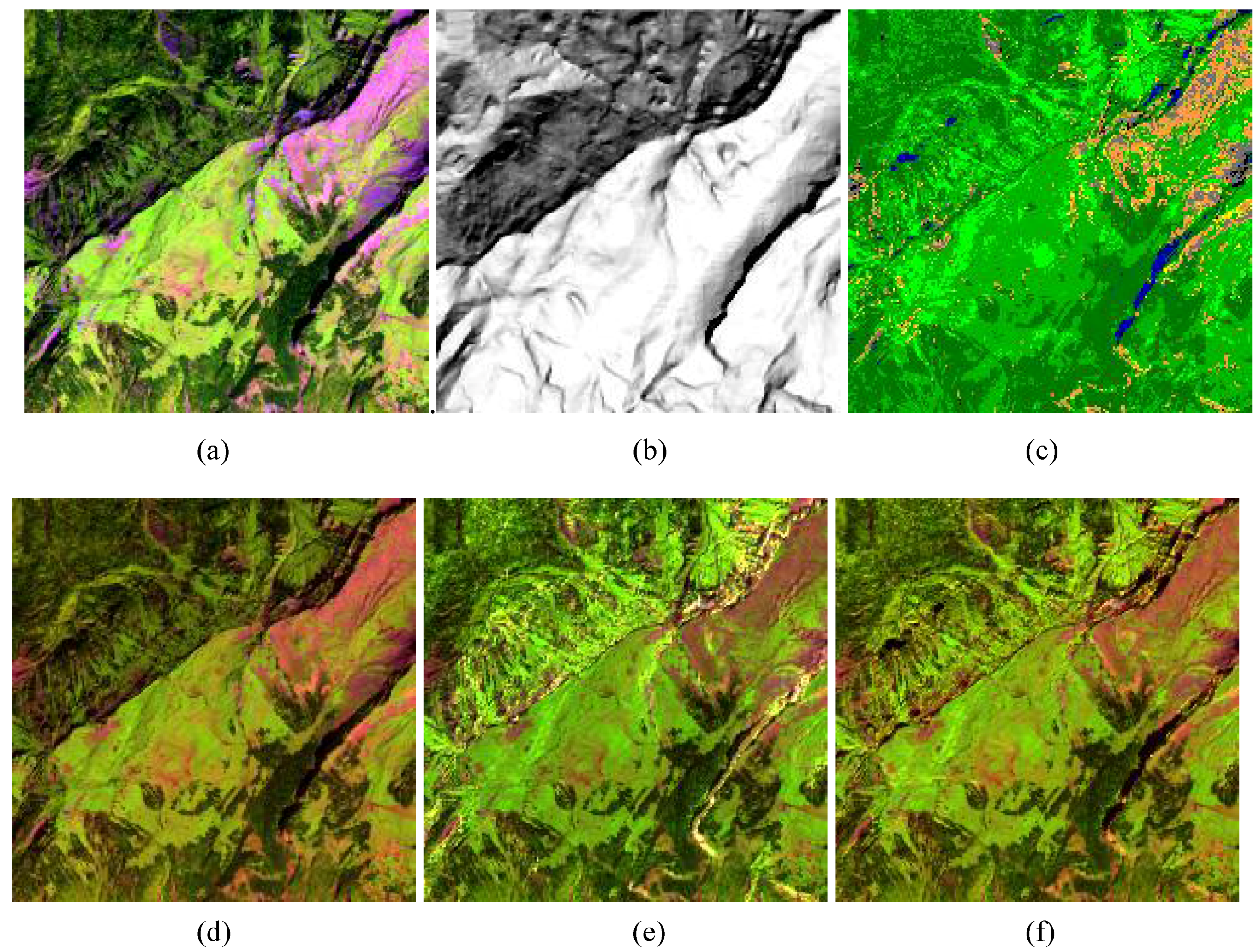
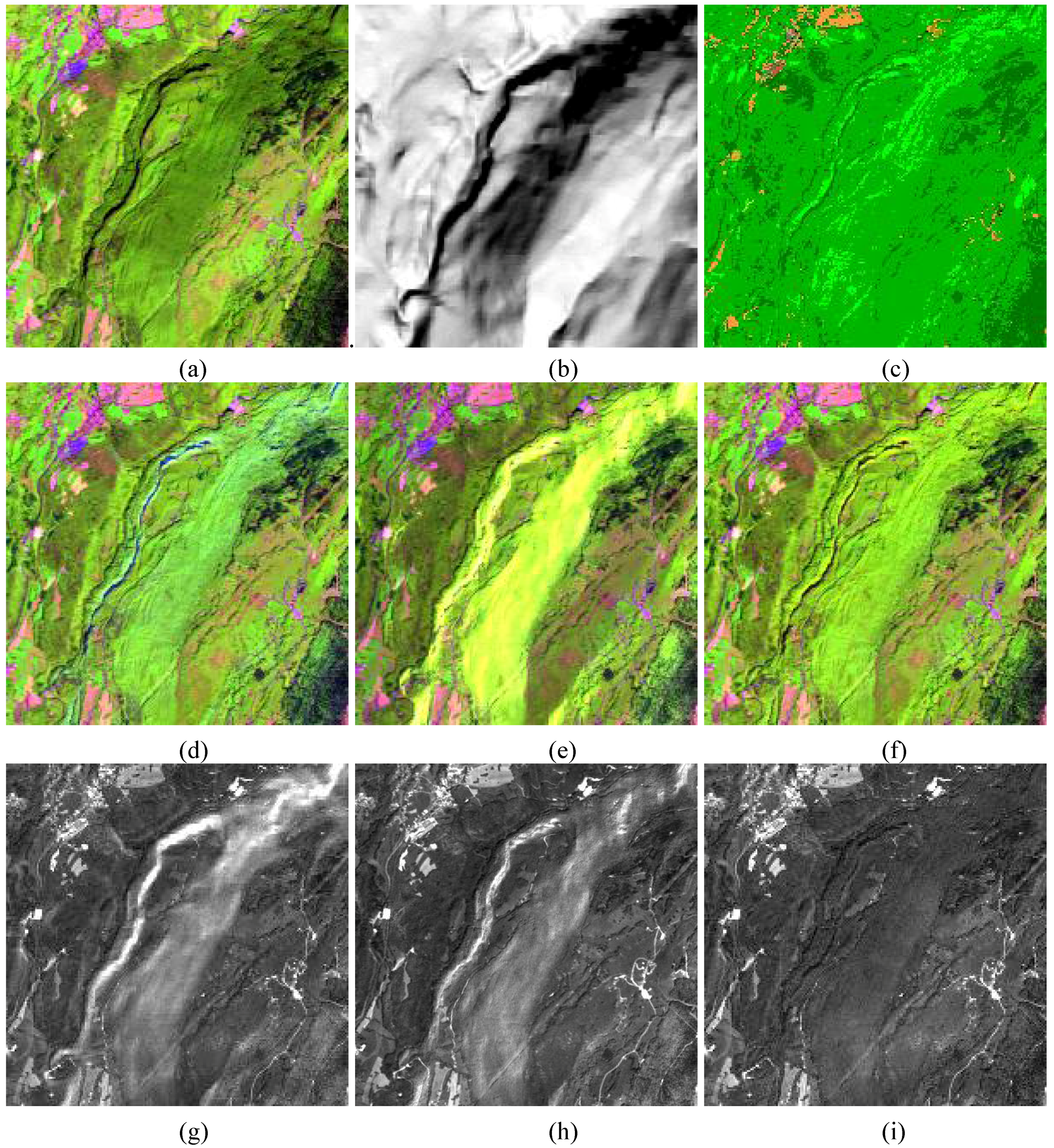
3.1. Scene (a)
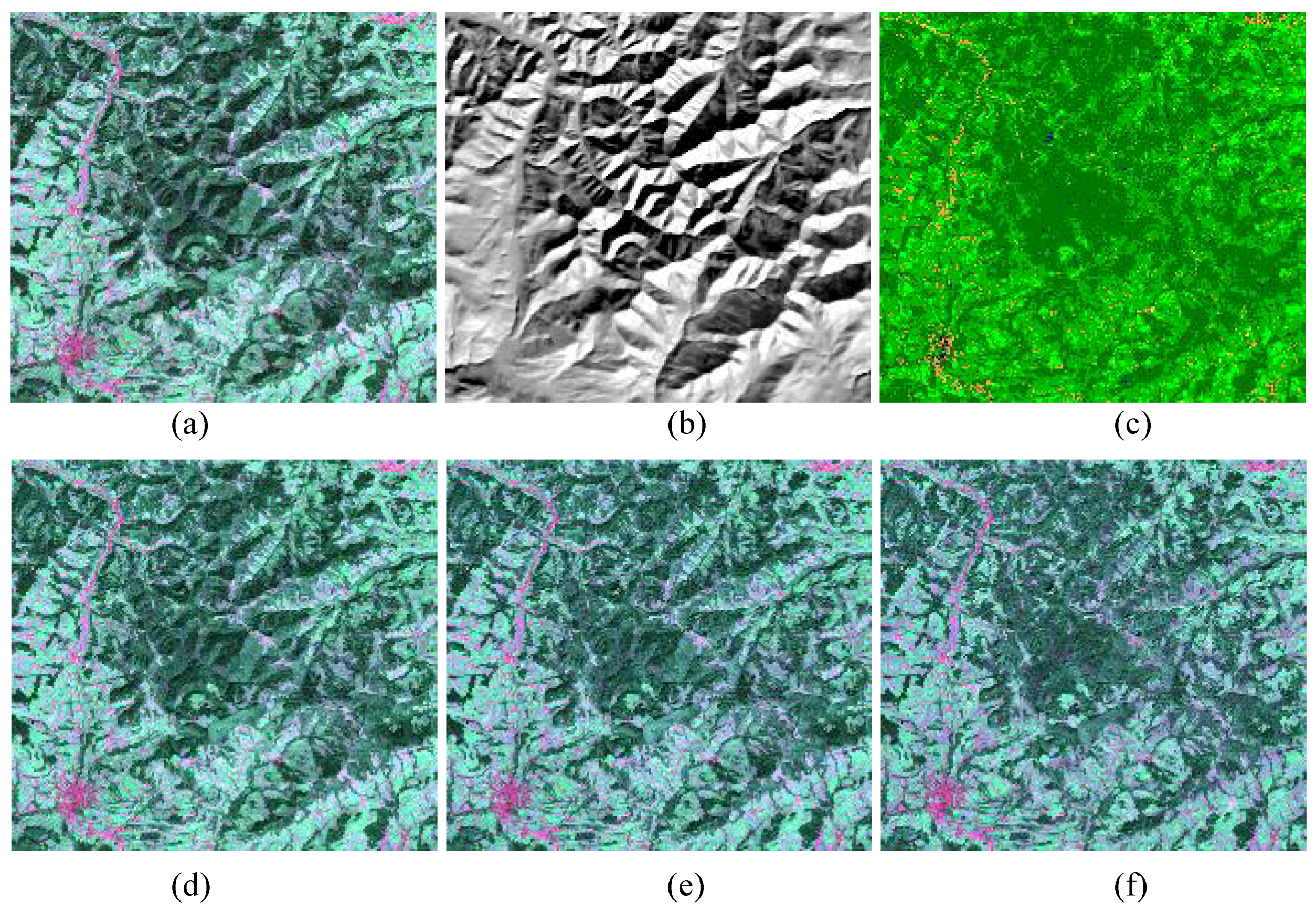
Figure 1 displays a sub-scene of the SPOT-5 scene (a). It has the largest off-nadir viewing angle (26.8°) of all considered scenes. Elevations range between 300 m and 1700 m, slopes between 0° and 42°. The illumination map (cosβ) represents the cosine of the local solar zenith angle and incorporates the topography. Bright areas receive a high illumination, dark areas are the critical ones, representing steep slopes oriented away from the sun. Therefore, the methods will likely yield different results in those dark areas. This can indeed be observed when comparing
Figure 1 (d) to (f). From the visual impression the MM method ranks first, followed by the C correction, Gamma ranks last, because of the large yellow areas in faintly illuminated regions. In the false colour image, the second rank of the C approach is not very clear, but the better performance of MM is obvious from the results of the first band, compare
Figure 1 (g) with (i). The classification map (
Figure 1 (c)) presents class1 (coniferous, coded as dark green), and class 2 (deciduous and agricultural, coded medium green). A comparison of
Figure 1 (b) and
Figure 1 (c) shows that the classification is only marginally dependent on the illumination.
Figure 1.
Sub-scene of (a), RGB = bands 4, 3, 2 (1650, 840, 660 nm). (a) Original. (b) Illumination. (c) Classification map. (d) C correction. (e) Gamma correction. (f) MM correction, (g) C (band 1). (h) Gamma (band 1). (i) MM (band 1).
Figure 1.
Sub-scene of (a), RGB = bands 4, 3, 2 (1650, 840, 660 nm). (a) Original. (b) Illumination. (c) Classification map. (d) C correction. (e) Gamma correction. (f) MM correction, (g) C (band 1). (h) Gamma (band 1). (i) MM (band 1).
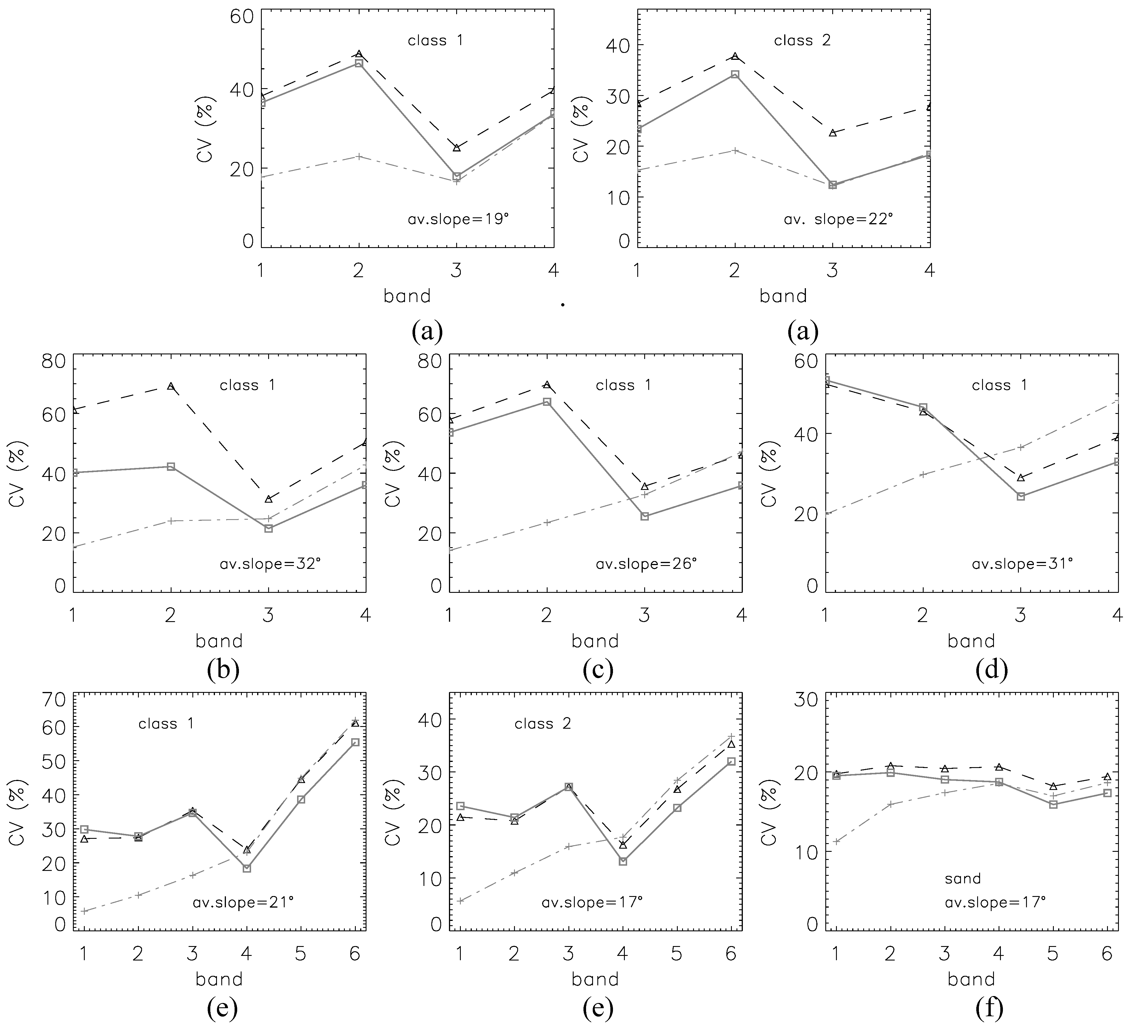
Figure 7 (a) presents the CV values for the classes 1 and 2. The average slope values are 19° (class 1) and 22° (class 2), not counting pixels in the flat plane. As low values indicate the best elimination of topographic features, the C method ranks first for the visible bands (1, 2), while C and MM achieve the same quality for the NIR and SWIR bands (3, 4). However, the visual comparison of
Figure 1 (g),(i) clearly indicates a better performance of the MM algorithm.
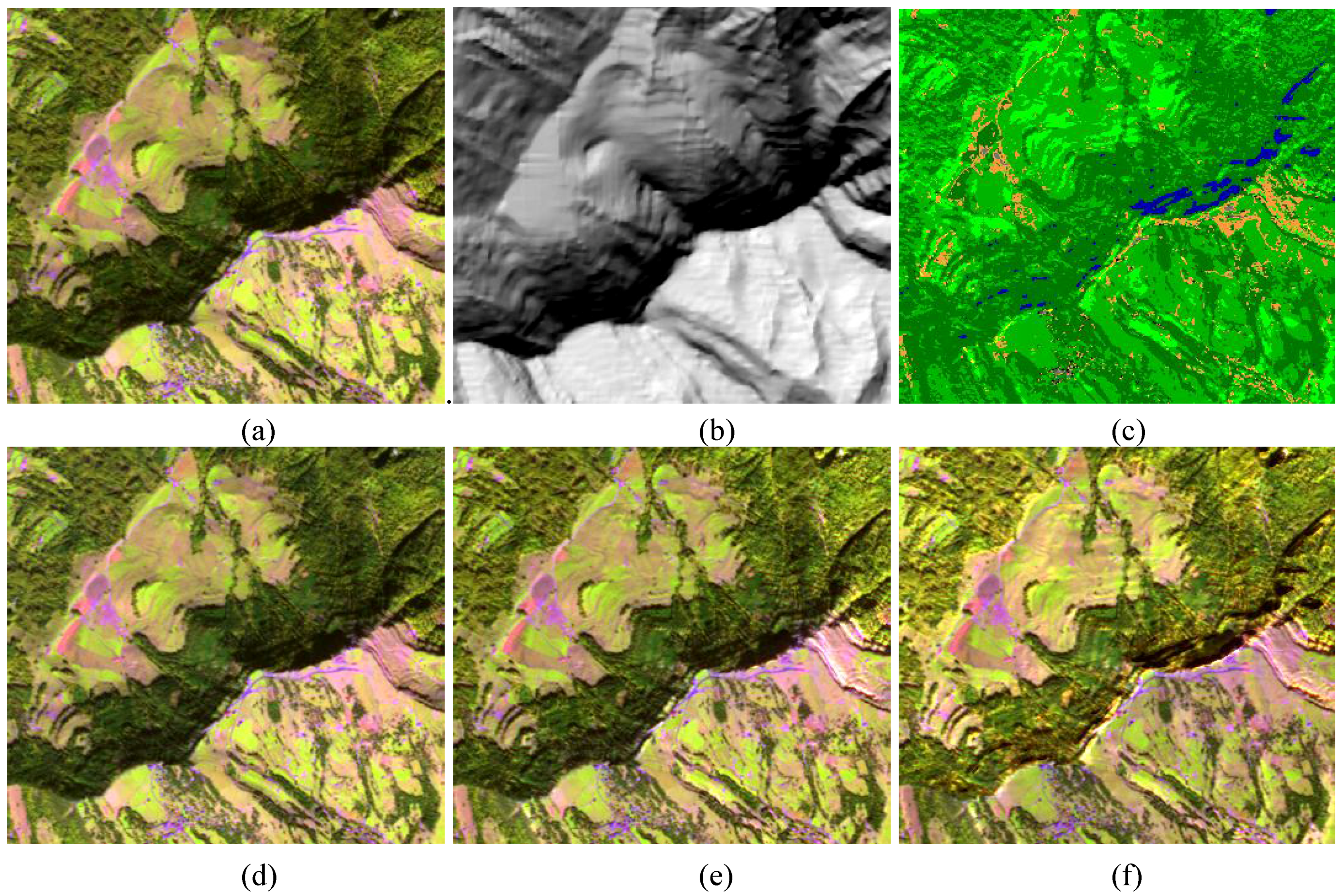
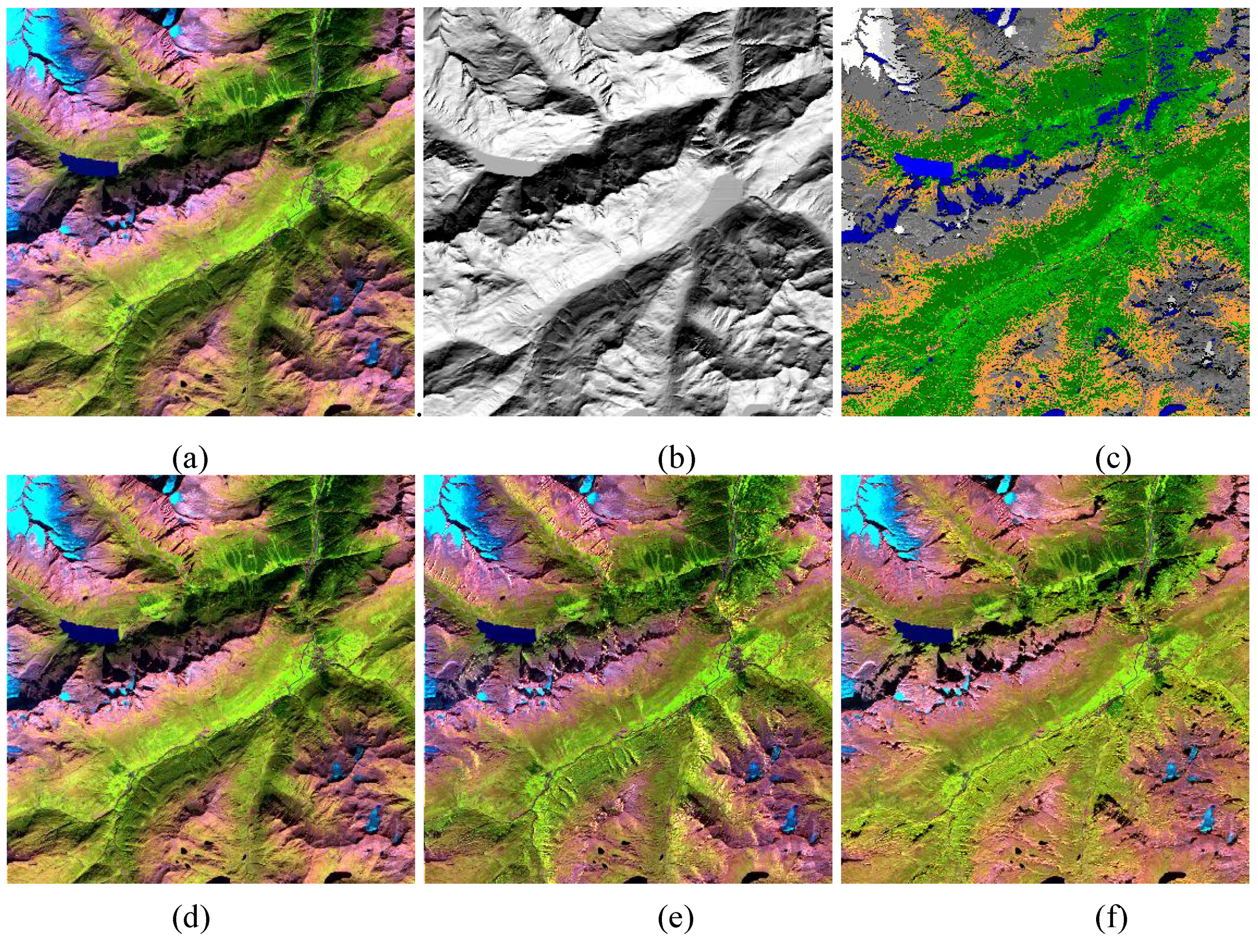
3.2. Scene (b)
Figure 2 displays a sub-scene of the SPOT-5 scene (b). It has a medium off-nadir viewing angle (13.2°). Elevations range between 600 m and 3,600 m, slopes between 0° and 64°. From the visual impression the MM method ranks first, followed by the Gamma, then the C algorithm. The Gamma image contains artifacts (yellow pixels) which do not appear in the MM corrected scene.
Figure 7 (b) presents the CV values for class 1. Results for class 2 show a similar trend, therefore, they are not included. The average slope of the terrain is 32°, not counting pixels in the flat plane, which is rather high. Again, for the visible bands (1, 2) the C method (+ symbol) ranks first, followed by MM, and Gamma. For the NIR, SWIR bands the ranking is MM, C, Gamma. However, the visual inspection places MM first for all bands.
Figure 2.
Sub-scene of (b), RGB = bands 4, 3, 2 (1650, 840, 660 nm). (a) Original. (b) Illumination. (c) Classification map. (d) C correction. (e) Gamma. (f) MM correction.
Figure 2.
Sub-scene of (b), RGB = bands 4, 3, 2 (1650, 840, 660 nm). (a) Original. (b) Illumination. (c) Classification map. (d) C correction. (e) Gamma. (f) MM correction.
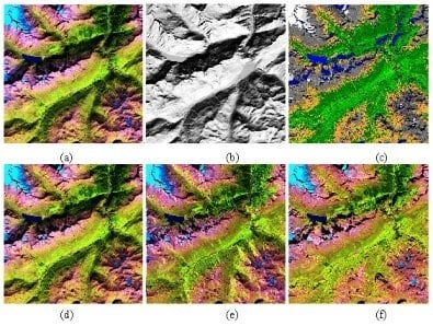
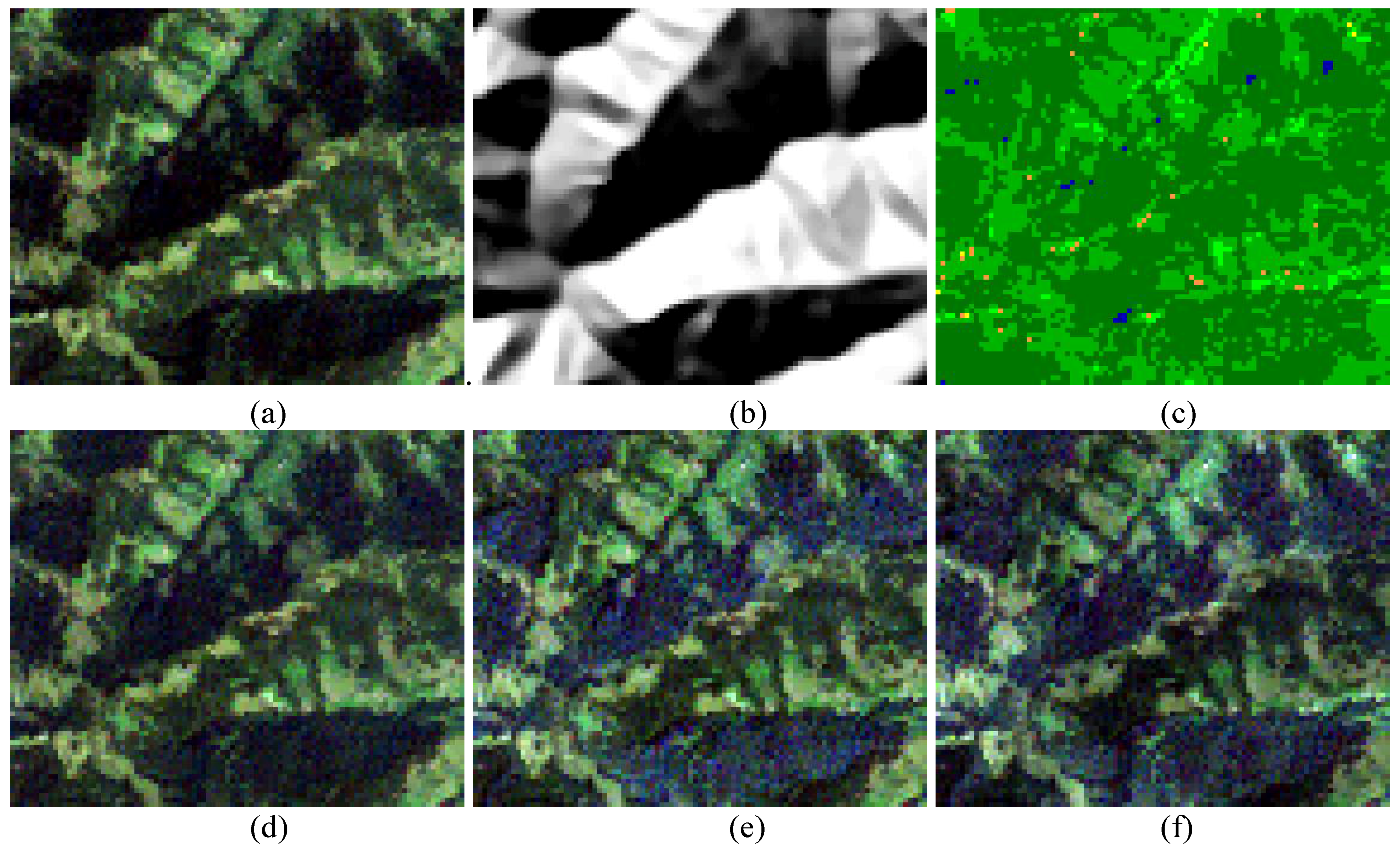
3.3. Scene (c)
Figure 3 displays a sub-scene of the SPOT-5 scene (c). It has a medium off-nadir viewing angle (15.7°). Elevations range from 400 m to 1900 m, and steep slopes up to 50° can be found. A comparison of the illumination (
Figure 3b) and classification maps (
Figure 3c) shows no correlation of class assignment and terrain illumination except for some blue areas (topographic shadow, misclassified as water) that do not belong to the evaluated classes 1 (dark green) and 2 (medium green). From the visual impression the MM method ranks first, followed by the Gamma, then the C algorithm.
Figure 7 (c) presents the CV values for class 1. Results for class 2 show a similar trend, therefore, they are not included. The average slope of the terrain is 26°. Again, for the visible bands (1, 2) the C method (+ symbol) ranks first, followed by MM, and Gamma. For the NIR, SWIR bands the ranking is MM, C, Gamma. However, the visual inspection places MM first for all bands.
Figure 3.
Sub-scene of (c), RGB = bands 4, 3, 2 (1650, 840, 660 nm). (a) Original. (b) Illumination. (c) Classification. (d) C correction. (e) Gamma correction. (f) MM correction.
Figure 3.
Sub-scene of (c), RGB = bands 4, 3, 2 (1650, 840, 660 nm). (a) Original. (b) Illumination. (c) Classification. (d) C correction. (e) Gamma correction. (f) MM correction.
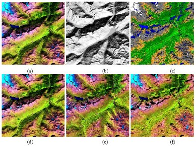
3.4. Scene (d)
Figure 4 displays a sub-scene of the SPOT-5 scene (d). It has a near-nadir viewing angle (2.3°). Elevations range between 1,200 m and 3,000 m, and steep slopes up to 58°. In the classification map of
Figure 4c some misclassifications occur in regions where the illumination is 0 (topographic shadow), see the blue areas indicating water bodies. However, these pixels are not used in the evaluation, and the vegetation classes 1 and 2 are correctly assigned. From the visual impression the MM method again ranks first, followed by the Gamma, then the C algorithm.
Figure 7 (d) presents the CV values for class 1. Results for class 2 show a similar trend, therefore, they are not included. The average slope of the terrain is 21°, not considering the flat terrain. Again, for the visible bands (1, 2) the C method ranks first, MM and Gamma values are nearly the same. For the NIR, SWIR bands the ranking is MM, Gamma, C. However, the visual inspection clearly places MM first for all bands.
Figure 4.
Sub-scene of (d), RGB = bands 4, 3, 2 (1650, 840, 660 nm). (a) Original. (b) Illumination. (c) Classification. (d) C correction. (e) Gamma correction. (f) MM correction.
Figure 4.
Sub-scene of (d), RGB = bands 4, 3, 2 (1650, 840, 660 nm). (a) Original. (b) Illumination. (c) Classification. (d) C correction. (e) Gamma correction. (f) MM correction.
3.5. Scene (e)
Figure 5 (a) and
Figure 5 (b) display two different sub-scenes of the Landsat-7 ETM+ scene (e). The scene was orthorectified with a Swisstopo 25 m DEM scaled to 30 m. Elevations range between 400 m and 1,100 m, slopes reach values up to 34°. The reason for selecting two sub-scenes is to demonstrate that the best performance ranking can even change from one sub-scene to the next within the same large scene. In the true colour image of
Figure 5a, the visual impression indicates that the best performance in suppressing topographic features is achieved with the C method, followed by MM, and Gamma. However, in the second sub-scene of
Figure 5 (b) with the NIR and SWIR bands the ranking is MM, followed by Gamma, then the C algorithm, while the true colour image (not shown for space reasons) yields the ranking MM, C, Gamma.
Figure 7 (e) presents the CV values for classes 1 and 2. The C method ranks first for the visible bands (1, 2, 3) while MM is superior for the NIR and SWIR bands. CV values for class 1 (conifers) are higher than for class 2 (deciduous forests, agricultural fields), because the mean reflectance values are lower for class 1, especially in the NIR and SWIR region, i.e., for the same standard deviation σ the
CV = 100 σ / mean will be larger.
Figure 5a.
Sub-scene 1 of (e), RGB = bands 3, 2, 1 at 660, 560, 480 nm. (a) Original. (b) Illumination. (c) Classification. (d) C correction. (e) Gamma correction. (f) MM correction.
Figure 5a.
Sub-scene 1 of (e), RGB = bands 3, 2, 1 at 660, 560, 480 nm. (a) Original. (b) Illumination. (c) Classification. (d) C correction. (e) Gamma correction. (f) MM correction.
Figure 5b.
Sub-scene 2 of (e), RGB = bands 7, 4, 5 (2200, 840, 1600 nm). (a) Original. (b) Illumination. (c) Classification. (d) C correction. (e) Gamma correction. (f) MM correction.
Figure 5b.
Sub-scene 2 of (e), RGB = bands 7, 4, 5 (2200, 840, 1600 nm). (a) Original. (b) Illumination. (c) Classification. (d) C correction. (e) Gamma correction. (f) MM correction.
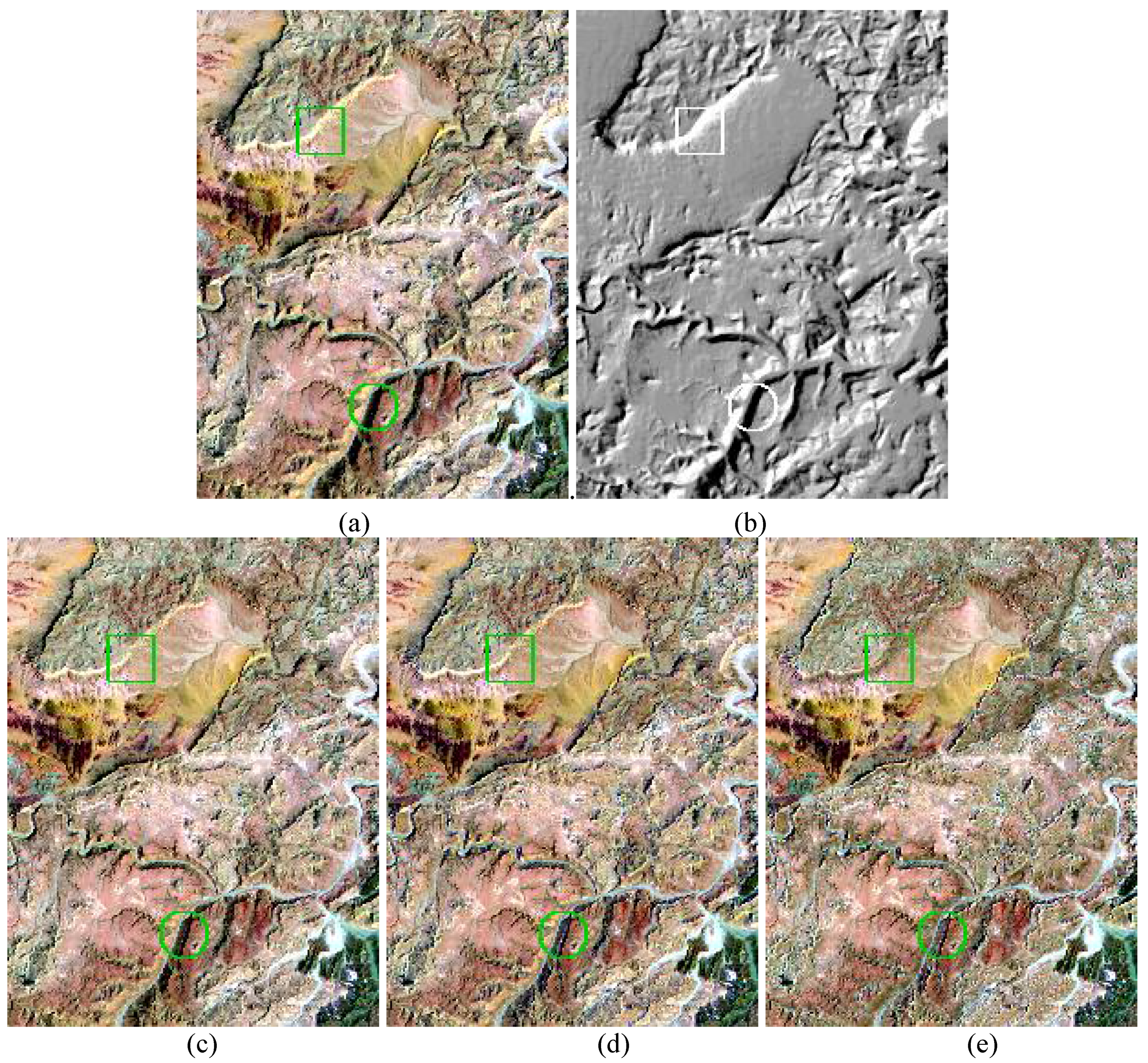
3.6. Scene (f)
Figure 6 shows a sub-scene of Landsat-5 TM from the Makhtesh Ramon area in Israel. The scene was orthorectified with a 25 m DEM scaled to 30 m. Elevations range between 200 m and 800 m, slope values reach 31°. The classification map is not shown as it contains only the sand class and no vegetation. Two locations have been marked in the image: the center of the square symbol shows pixels oriented to the sun [bright in
Figure 6 (b)], and the center of the circle indicates pixels oriented away from the sun [dark in
Figure 6 (b)]. From the visual impression, the best performance in eliminating topographic features is achieved with the MM algorithm, followed by Gamma, then the C method. Although only one RGB band combination is shown here for space reasons, this statement holds true for all band combinations.
Figure 6.
Sub-scene of (f), RGB = bands 7, 4, 1 (2200, 840, 480 nm. (a) Original. (b) Illumination. (c) C correction. (d) Gamma correction. (e) MM correction.
Figure 6.
Sub-scene of (f), RGB = bands 7, 4, 1 (2200, 840, 480 nm. (a) Original. (b) Illumination. (c) C correction. (d) Gamma correction. (e) MM correction.
Figure 7 (f) presents the CV values for the six reflective bands of TM. For the selected arid region, there exist only class 3 pixels (sand). Similar to the previous results with the SPOT-5 and ETM+ scenes, the C method has the best performance in the visible bands. The MM algorithm again ranks first in the NIR and SWIR bands. In
Figure 7, for scenes (b), (c), (d) results are only shown for class 1 because those for class 2 are very similar. Scene (f) has no vegetation, so only class 3 (sand) is displayed.
Figure 7.
Coefficient of variation (CV) for each spectral band. (a) to (f) correspond to scenes (a) to (f) of
Table 1. The symbols +, square, and triangle mark results of the C, MM, and Gamma method, respectively. Band 6 for TM and ETM+ represents the 6
th reflective band at 2.2 µm (also known as Landsat band 7).
A remark concerning TOA reflectance (C method) and surface reflectance (Gamma and MM): the use of TOA reflectance has no adverse effect on the visual appearance. However, as the TOA reflectance in the visible bands usually is higher than the surface reflectance (because of the path radiance contribution) the TOA CV values are lower than the surface reflectance CV values. As the standard deviation for both reflectance products is about the same, the TOA CV values are biased toward lower values. However, this “advantage” is lost if the C method is applied to surface reflectance data. An additional slight advantage of the TOA reflectance for the CV evaluation is the smoothing low pass filter effect of the atmosphere which yields somewhat smaller standard deviations compared to the surface reflectance product. According to the recommendation of [
6] we also investigated the performance of the C method with a smoothed DEM slope map, i.e., using a kernel of 5 × 5 pixels during the calculation of the slope/aspect maps. However, no improvement was achieved for our scenes.
Table 2 shows a summary of all assessments (visual, CV, overall) for all scenes. The overall best rankings are achieved with the MM method.
Table 2.
Rankings for all scenes.
Table 2.
Rankings for all scenes.
| | Visual Assessment | CV | |
|---|
| Scene ID | VIS | NIR / SWIR | VIS | NIR / SWIR | Overall |
|---|
| A | MM | MM | C | MM | MM |
| B | MM | MM | C | MM | MM |
| C | MM | MM | C | MM | MM |
| D | MM | MM | C | MM | MM |
| E | C | MM | C | MM | MM |
| F | MM | MM | C | MM | MM |


