Sustainability in the Food-Water-Ecosystem Nexus: The Role of Land Use and Land Cover Change for Water Resources and Ecosystems in the Kilombero Wetland, Tanzania

 , ,
, ,
Abstract
:1. Introduction
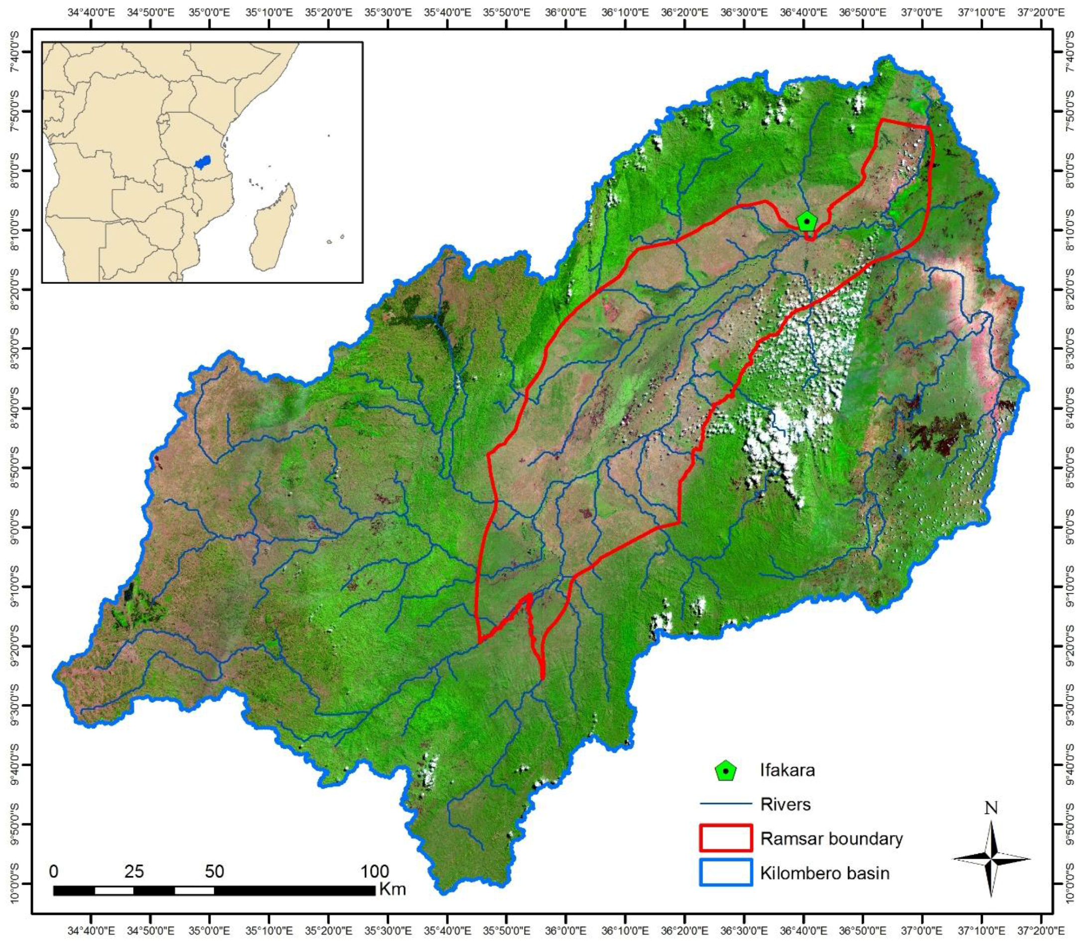
2. Study Site
3. Methods
3.1. Land Use and Land Cover Classification and Change Assessment
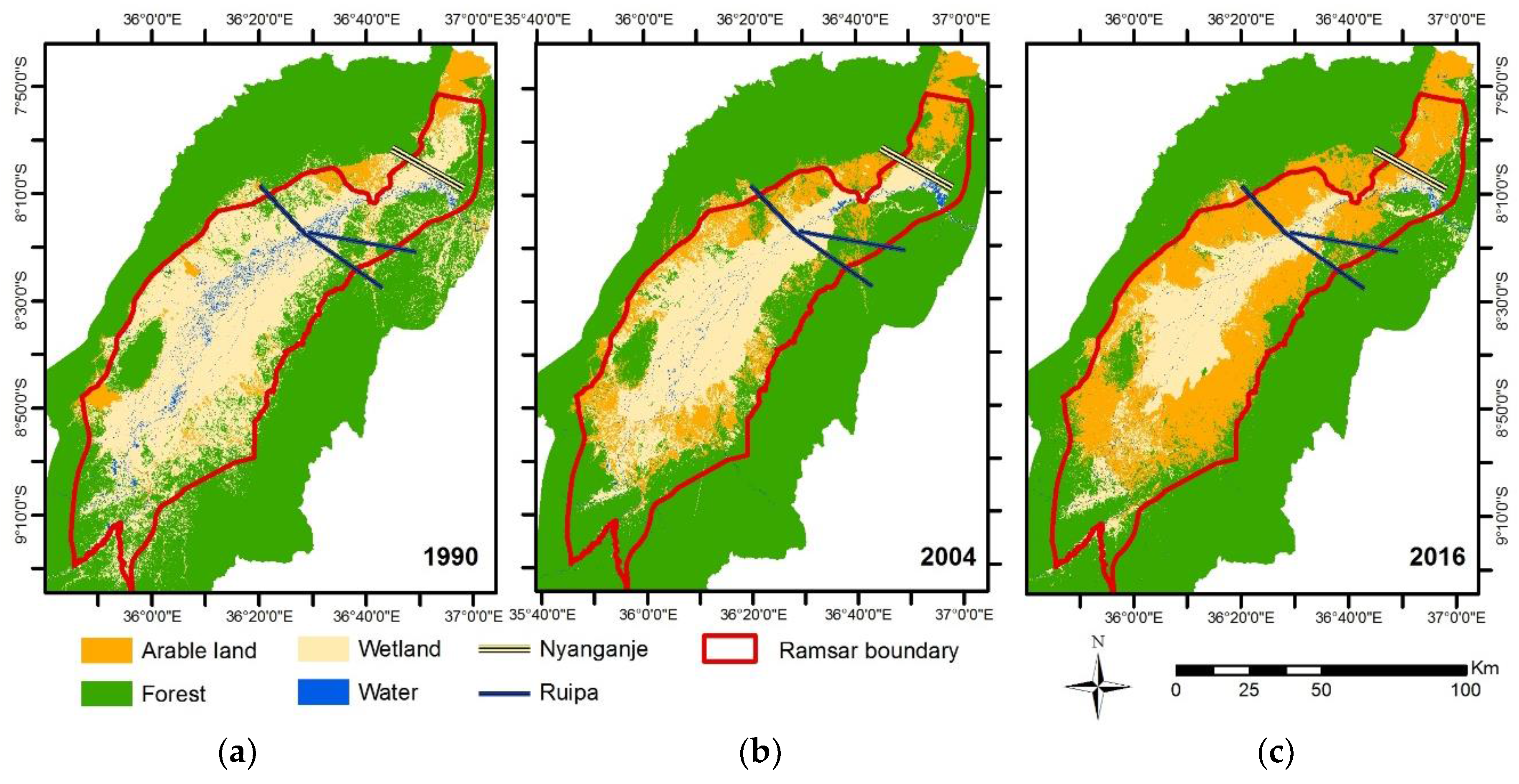
3.1.1. LULC Changes in the Kilombero Floodplain
3.1.2. LULC Changes at the Catchment Scale
3.2. The Impact of Land Use and Land Cover on Water Resources at the Catchment Scale
3.2.1. The SWAT Model Setup for the Kilombero Catchment
3.2.2. Model Configuration and Performance Evaluation
4. Results
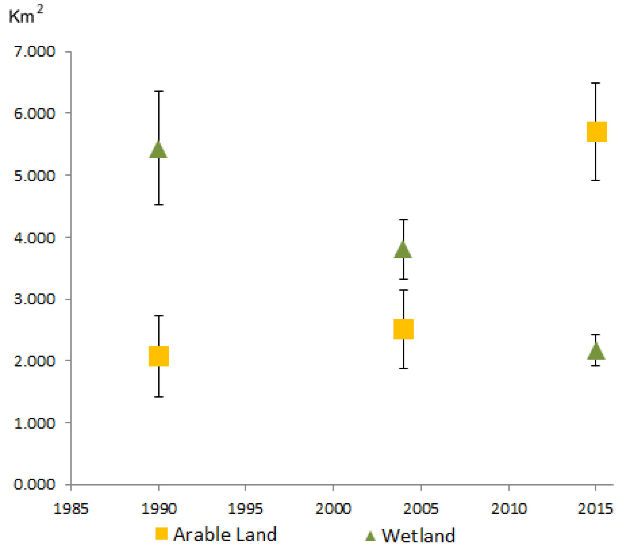
4.1. LULCC at Floodplain Scale
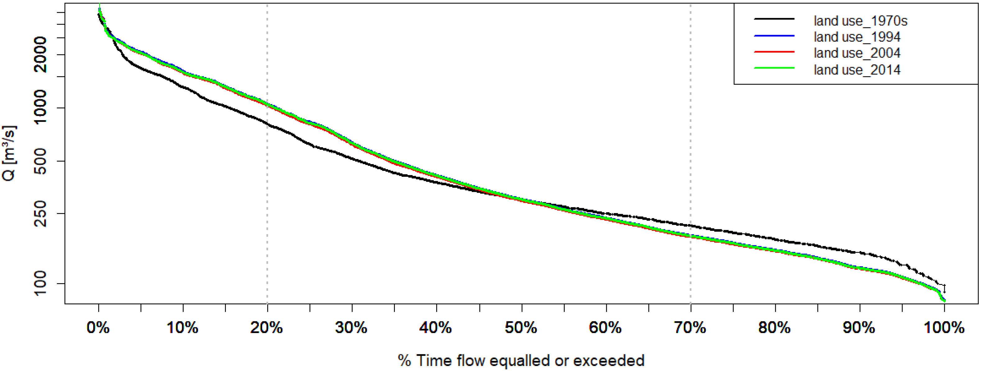
4.2. LULC Changes at the Catchment Scale
5. Discussion
5.1. The Potential, Uncertainties and Limitations of LULCC Analysis and SWAT Application
5.2. Science-Policy Interface and Capacity Building
6. Conclusions—Ways Forward
Acknowledgments
Author Contributions
Conflicts of Interest
References
- Finlayson, C.M.; Davis, J.A.; Gell, P.A.; Kingsford, R.T.; Parton, K.A. The status of wetlands and the predicted effects of global climate change: The situation in Australia. Aquat. Sci. 2013, 75, 73–93. [Google Scholar] [CrossRef]
- Junk, W.J.; An, S.; Finlayson, C.M.; Gopal, B.; Květ, J.; Mitchell, S.A.; Mitsch, W.J.; Robarts, R.D. Current state of knowledge regarding the world’s wetlands and their future under global climate change: A synthesis. Aquat. Sci. 2013, 75, 151–167. [Google Scholar] [CrossRef]
- Zedler, J.B.; Kercher, S. Wetland Resources: Status, Trends, Ecosystem Services, and Restorability. Annu. Rev. Environ. Resour. 2005, 30, 39–74. [Google Scholar] [CrossRef]
- Mooney, H.A.; Cropper, A.; Leemans, R.; Arico, S.; Bridgewater, P.; Peterson, G.; Revenga, C.; Rivera, M. Millenium Ecosystem Assessment. In Ecosystems and Human Well-Being: Wetlands and Water Synthesis; World Resource Institute: Washington, DC, USA, 2005; ISBN 156-9-73-597-2. Available online: https://www.millenniumassessment.org/documents/document.358.aspx.pdf (accessed on 23 August 2017).
- Lawford, R.; Strauch, A.; Toll, D.; Fekete, B.; Cripe, D. Earth observations for global water security. Curr. Opin. Environ. Sustain. 2013, 5, 633–643. [Google Scholar] [CrossRef]
- Kansakar, P.; Hossain, F. A review of applications of satellite earth observation data for global societal benefit and stewardship of planet earth. Space Policy 2016, 36, 46–54. [Google Scholar] [CrossRef]
- Von der Heyden, C.; New, M.G. The role of a dambo in the hydrology of a catchment and the river network downstream. Hydrol. Earth Syst. Sci. 2003, 7, 339–357. [Google Scholar] [CrossRef]
- Piao, S.; Friedlingstein, P.; Ciais, P.; de Noblet-Ducoudré, N.; Labat, D.; Zaehle, S. Changes in climate and land use have a larger direct impact than rising CO2 on global river runoff trends. Proc. Natl. Acad. Sci. USA 2007, 104, 15242–15247. [Google Scholar] [CrossRef] [PubMed]
- Hoff, H.; Falkenmark, M.; Gerten, D.; Gordon, L.; Karlberg, L.; Rockström, J. Greening the global water system. J. Hydrol. 2010, 384, 177–186. [Google Scholar] [CrossRef]
- Falkenmark, M.; Molden, D. Wake Up to Realities of River Basin Closure. Int. J. Water Resour. Dev. 2008, 24, 201–215. [Google Scholar] [CrossRef]
- Machingura, F.; Lally, S. Case Study Report the Sustainable Development Goals and Their Trade-Offs; Overseas Development Institute: London, UK , 2017; Available online: https://www.odi.org/sites/odi.org.uk/files/resource-documents/11329.pdf (accessed on 23 August 2017).
- Bhaduri, A.; Bogardi, J.J.; Siddiqi, A.; Voigt, H.; Vörösmarty, C.; Pahl-Wostl, C.; Bunn, S.; Shrivastava, P.; Lawford, R.; Foster, S.; et al. Achieving Sustainable Development Goals from a Water Perspective. Front. Environ. Sci. 2016, 4, 1–13. [Google Scholar] [CrossRef]
- Ait-kadi, M. Water for Development and Development for Water: Realizing the Sustainable Development Goals (SDGs) Vision. Aquat. Procedia 2016, 6, 106–110. [Google Scholar] [CrossRef]
- Bhaduri, A.; Ringler, C.; Dombrowski, I.; Mohtar, R.; Scheumann, W. Sustainability in the water-energy-food nexus. Water Int. 2015, 40, 723–732. [Google Scholar] [CrossRef]
- Mcclain, M.E. Balancing Water Resources Development and Environmental Sustainability in Africa: A Review of Recent Research Findings and Applications. Ambio 2013, 42, 549–565. [Google Scholar] [CrossRef] [PubMed]
- Vörösmarty, C.J.; Green, P.; Salisbury, J.; Lammers, R.B. Global Water Resources: Vulnerability from Climate Change and Population Growth. Science 2000, 289, 284–288. [Google Scholar] [CrossRef] [PubMed]
- Liu, J.; Yang, H. Spatially explicit assessment of global consumptive water uses in cropland: Green and blue water. J. Hydrol. 2010, 384, 187–197. [Google Scholar] [CrossRef]
- Cornelissen, T.; Diekkrüger, B.; Giertz, S. A comparison of hydrological models for assessing the impact of land use and climate change on discharge in a tropical catchment. J. Hydrol. 2013, 498, 221–236. [Google Scholar] [CrossRef]
- Siebert, S.; Döll, P. Quantifying blue and green virtual water contents in global crop production as well as potential production losses without irrigation. J. Hydrol. 2010, 384, 198–217. [Google Scholar] [CrossRef]
- Amler, E.; Schmidt, M.; Menz, G. Definitions and Mapping of East African Wetlands: A Review. Remote Sens. 2015, 7, 5256–5282. [Google Scholar] [CrossRef]
- MacKay, H.; Finlayson, C.M.; Fernández-Prieto, D.; Davidson, N.; Pritchard, D.; Rebelo, L.-M. The role of Earth Observation (EO) technologies in supporting implementation of the Ramsar Convention on Wetlands. J. Environ. Manag. 2009, 90, 2234–2242. [Google Scholar] [CrossRef] [PubMed]
- Cetin, M. Sustainability of urban coastal area management: A case study on Cide. J. Sustain. For. 2016, 35, 527–541. [Google Scholar] [CrossRef]
- Brink, A.B.; Eva, H.D. Monitoring 25 years of land cover change dynamics in Africa: A sample based remote sensing approach. Appl. Geogr. 2009, 29, 501–512. [Google Scholar] [CrossRef]
- Maitima, J.M.; Mugatha, S.M.; Reid, R.S.; Gachimbi, L.N.; Majule, A.; Lyaruu, H.; Pomery, D.; Mathai, S.; Mugisha, S. The linkages between land use change, land degradation and biodiversity across East Africa. Afr. J. Environ. Sci. Technol. 2009, 3, 310–325. [Google Scholar]
- Brink, A.B.; Bodart, C.; Brodsky, L.; Defourney, P.; Ernst, C.; Donney, F.; Lupi, A.; Tuckova, K. Anthropogenic pressure in East Africa—Monitoring 20 years of land cover changes by means of medium resolution satellite data. Int. J. Appl. Earth Obs. Geoinf. 2014, 28, 60–69. [Google Scholar] [CrossRef]
- Kashaigili, J.J.; Majaliwa, A.M. Integrated assessment of land use and cover changes in the Malagarasi river catchment in Tanzania. Phys. Chem. Earth Parts A/B/C 2010, 35, 730–741. [Google Scholar] [CrossRef]
- Kashaigili, J.J. Impacts of land-use and land-cover changes on flow regimes of the Usangu wetland and the Great Ruaha River, Tanzania. Phys. Chem. Earth Parts A/B/C 2008, 33, 640–647. [Google Scholar] [CrossRef]
- Msoffe, F.U.; Said, M.Y.; Ogutu, J.O.; Kifugo, S.C.; de Leeuw, J.; van Gardingen, P.; Reid, R.S. Spatial correlates of land-use changes in the Maasai-Steppe of Tanzania: Implications for conservation and environmental planning. Int. J. Biodivers. Conserv. 2011, 3, 280–290. [Google Scholar]
- Msuha, M.J.; Carbone, C.; Pettorelli, N.; Durant, S.M. Conserving biodiversity in a changing world: Land use change and species richness in northern Tanzania. Biodivers. Conserv. 2012, 21, 2747–2759. [Google Scholar] [CrossRef]
- Milder, J.C.; Hart, A.K.; Buck, L.E. Applying an Agriculture Green Growth Approach in the SAGCOT Clusters: Challenges and Opportunities in Kilombero, Ihemi and Mbarali; SAGCOT Centre: Dar es Salaam, Tanzania, 2013. [Google Scholar]
- Government of Tanzania Southern Agricultural Growth Corridor of Tanzania (SAGCOT): Environmental and Social Management Framework (ESMF); Environmental Resources Management Limited: Dar es Salaam, Tanzania, 2013; pp. 1–175. Available online: http://www.sagcot.com/uploads/media/SAGCOT_Final_ESMF_For_Redisclosure_20_August_2013.pdf (accessed on 23 August 2017).
- Leemhuis, C.; Amler, E.; Diekkrüger, B.; Gabiri, G.; Näschen, K. East African wetland-catchment data base for sustainable wetland management. Proc. Int. Assoc. Hydrol. Sci. 2016, 374, 123–128. [Google Scholar] [CrossRef]
- Mombo, F.; Speelman, S.; Huylenbroeck, G.; Van Hella, J.; Moe, S. Ratification of the Ramsar convention and sustainable wetlands management: Situation analysis of the Kilombero Valley wetlands in Tanzania. JAERD 2011, 3, 153–164. [Google Scholar]
- Beck, A.D. The Kilombero valley of south-central Tanganyika. East Afr. Geogr. Rev. 1964, 1964, 37–43. Available online: https://journals.co.za/content/eagr/1964/2/AJA19376812_7 (accessed on 23 August 2017).
- Koutsouris, A.J.; Chen, D.; Lyon, S.W. Comparing global precipitation data sets in eastern Africa: A case study of Kilombero Valley, Tanzania. Int. J. Climatol. 2016, 36, 2000–2014. [Google Scholar] [CrossRef]
- RBWO. The Rufiji Basin Water Office (RBWO) Discharge Database; RBWO: Iringa, Tanzania, 2014; Available online: http://rbwo.org (accessed on 23 August 2017).
- National Bureau of Statistics 2012 Census Data. Available online: http://dataforall.org/dashboard/tanzania/ (accessed on 8 April 2017).
- Monson, J. Freedom Railway: How a Chinese Development Project Changed Lives and Livelihoods in Tanzania; Indiana University Press: St Bloomington, IN, USA, 2009. [Google Scholar]
- Hughes, R.H.; Hughes, J.S. A Directory of African Wetlands; IUCN: Gland, Switzerland, 1992; ISBN 978-2-88-032949-5. [Google Scholar]
- Siima, S.B.; Munishi, P.K.T.; Ngaga, Y.M.; Navrud, S. Estimating direct use value of Kilombero Ramsar Site based on market price method. Tanzan. J. For. Nat. Conserv. 2012, 81, 133–146. [Google Scholar]
- Nindi, S.J.; Maliti, H.; Bakari, S.; Kija, H.; Machoke, M. Conflicts Over Land and Water Resources in the Kilombero Valley Floodplain, Tanzania. Afr. Study Monogr. 2014, 50, 173–190. [Google Scholar] [CrossRef]
- Wilson, E.; McInnes, R.; Mbanga, D.P.; Ouedraogo, P. Ramsar Advisory Mission Report; Ramsar Site No. 1173; Kilombero Valley Teak Company Ltd: Dar es Salaam, Tanzania, 2017; Available online: http://www.ramsar.org/sites/default/files/documents/library/ram83_kilombero_valley_tanzania_2016_e.pdf (accessed on 23 August 2017).
- Drusch, M.; Del Bello, U.; Carlier, S.; Colin, O.; Fernandez, V.; Gascon, F.; Hoersch, B.; Isola, C.; Laberinti, P.; Martimort, P.; et al. Sentinel-2: ESA’s Optical High-Resolution Mission for GMES Operational Services. Remote Sens. Environ. 2012, 120, 25–36. [Google Scholar] [CrossRef]
- Hüttich, C.; Reschke, J.; Keil, M.; Dech, S.; Weise, K.; Beltrame, C.; Fitoka, H.; Paganini, M. Using the Landsat Archive for the Monitoring of Mediterranean Coastal Wetlands: Examples from the Glob-Wetland-II Project. Earthzine. 2011, pp. 1–10. Available online: https://earthzine.org/2011/12/20/using-the-landsat-archive-for-the-monitoring-of-mediterranean-coastal-wetlands-examples-from-the-globwetland-ii-project/ (accessed on 23 August 2017).
- Bey, A.; Sánchez-Paus Díaz, A.; Maniatis, D.; Marchi, G.; Mollicone, D.; Ricci, S.; Bastin, J.-F.; Moore, R.; Federici, S.; Rezende, M.; et al. Collect Earth: Land Use and Land Cover Assessment through Augmented Visual Interpretation. Remote Sens. 2016, 8, 807. [Google Scholar] [CrossRef]
- Olofsson, P.; Foody, G.M.; Herold, M.; Stehman, S.V.; Woodcock, C.E.; Wulder, M.A. Good practices for estimating area and assessing accuracy of land change. Remote Sens. Environ. 2014, 148, 42–57. [Google Scholar] [CrossRef]
- Jensen, J.R.; Ramsey, E.W.; Mackey, H.E.; Christensen, E.J.; Sharitz, R.R. Inland Wetland Change Detection Using Aircraft MSS Data. Photogramm. Eng. Remote Sens. 1987, 53, 521–529. [Google Scholar]
- Ozesmi, S.L.; Bauer, M.E. Satellite remote sensing of wetlands. Wetl. Ecol. Manag. 2002, 10, 381–402. [Google Scholar] [CrossRef]
- Muro, J.; Canty, M.; Conradsen, K.; Hüttich, C.; Nielsen, A.A.; Skriver, H.; Remy, F.; Strauch, A.; Thonfeld, F.; Menz, G. Short-Term Change Detection in Wetlands Using Sentinel-1 Time Series. Remote Sens. 2016, 8, 795. [Google Scholar] [CrossRef]
- Schmitt, A.; Brisco, B. Wetland Monitoring Using the Curvelet-Based Change Detection Method on Polarimetric SAR Imagery. Water 2013, 5, 1036–1051. [Google Scholar] [CrossRef]
- White, L.; Brisco, B.; Dabboor, M.; Schmitt, A.; Pratt, A. A Collection of SAR Methodologies for Monitoring Wetlands. Remote Sens. 2015, 7, 7615–7645. [Google Scholar] [CrossRef] [Green Version]
- Torres, R.; Snoeij, P.; Geudtner, D.; Bibby, D.; Davidson, M.; Attema, E.; Potin, P.; Rommen, B.; Floury, N.; Brown, M.; et al. GMES Sentinel-1 mission. Remote Sens. Environ. 2012, 120, 9–24. [Google Scholar] [CrossRef]
- Potin, P.; Bargellini, P.; Laur, H.; Rosich, B.; Schmuck, S. Sentinel-1 mission operations concept. In Proceedings of the 2012 IEEE International Geoscience and Remote Sensing Symposium, Munich, Germany, 22–27 July 2012; pp. 1745–1748. [Google Scholar]
- Mack, B.; Leinenkugel, P.; Kuenzer, C.; Dech, S. A semi-automated approach for the generation of a new land use and land cover product for Germany based on Landsat time-series and Lucas in-situ data. Remote Sens. Lett. 2017, 8, 244–253. [Google Scholar] [CrossRef]
- Masek, J.G.; Vermote, E.F.; Saleous, N.E.; Wolfe, R.; Hall, F.G.; Huemmrich, K.F.; Gao, F.; Kutler, J.; Lim, T.-K. A Landsat surface reflectance dataset for North America, 1990–2000. IEEE Geosci. Remote Sens. Lett. 2006, 3, 68–72. [Google Scholar] [CrossRef]
- Vermote, E.; Justice, C.; Claverie, M.; Franch, B. Preliminary analysis of the performance of the Landsat 8/OLI land surface reflectance product. Remote Sens. Environ. 2016, 185, 46–56. [Google Scholar] [CrossRef]
- Zhu, Z.; Wang, S.; Woodcock, C.E. Improvement and expansion of the Fmask algorithm: Cloud, cloud shadow, and snow detection for Landsats 4–7, 8, and Sentinel 2 images. Remote Sens. Environ. 2015, 159, 269–277. [Google Scholar] [CrossRef]
- Zhu, Z.; Woodcock, C.E. Object-based cloud and cloud shadow detection in Landsat imagery. Remote Sens. Environ. 2012, 118, 83–94. [Google Scholar] [CrossRef]
- Arnold, J.G.; Srinivasan, R.; Muttiah, R.S.; Williams, J.R. Large area hydrologic modeling and assessment part I: Model development. J. Am. Water Resour. Assoc. 1998, 34, 73–89. [Google Scholar] [CrossRef]
- Tucker, C.J. Red and photographic infrared linear combinations for monitoring vegetation. Remote Sens. Environ. 1979, 8, 127–150. [Google Scholar] [CrossRef]
- McFeeters, S.K. The use of the Normalized Difference Water Index (NDWI) in the delineation of open water features. Int. J. Remote Sens. 1996, 17, 1425–1432. [Google Scholar] [CrossRef]
- Crist, E.P.; Cicone, R.C. A Physically-Based Transformation of Thematic Mapper Data—The TM Tasseled Cap. IEEE Trans. Geosci. Remote Sens. 1984, GE-22, 256–263. [Google Scholar] [CrossRef]
- Crist, E.P. A TM Tasseled Cap equivalent transformation for reflectance factor data. Remote Sens. Environ. 1985, 17, 301–306. [Google Scholar] [CrossRef]
- Kauth, R.; Thomas, G. The Tasselled Cap—A Graphic Description of the Spectral-Temporal Development of Agricultural Crops as Seen by Landsat. In Proceedings of the Symposium on Machine Processing of Remotely Sensed Data, West Lafayette, IN, USA, 29 June–1 July 1976. [Google Scholar]
- Yamamoto, K.H.; Finn, M.P. Approximating Tasseled Cap Values to Evaluate Brightness, Greenness, and Wetness for the Advanced Land Imager (ALI); Scientific Investigations Report; U.S. Geological Survey: Reston, VA, USA, 2012.
- Beven, K.J.; Kirkby, M.J. A physically based, variable contributing area model of basin hydrology/Un modèle à base physique de zone d’appel variable de l’hydrologie du bassin versant. Hydrol. Sci. Bull. 1979, 24, 43–69. [Google Scholar] [CrossRef]
- Breiman, L. Using Adaptive Bagging to Debias Regressions; Technical Report 547; Statistics Deptartment UCB: Berkeley, CA, USA, 1999. [Google Scholar]
- Breiman, L. Random forests. Mach. Learn. 2001, 45, 5–32. [Google Scholar] [CrossRef]
- Pal, M. Random forest classifier for remote sensing classification. Int. J. Remote Sens. 2005, 26, 217–222. [Google Scholar] [CrossRef]
- Rokach, L. Ensemble-based classifiers. Artif. Intell. Rev. 2010, 33, 1–39. [Google Scholar] [CrossRef]
- Gessner, U.; Machwitz, M.; Esch, T.; Tillack, A.; Naeimi, V.; Kuenzer, C.; Dech, S. Multi-sensor mapping of West African land cover using MODIS, ASAR and TanDEM-X/TerraSAR-X data. Remote Sens. Environ. 2015, 164, 282–297. [Google Scholar] [CrossRef]
- Ghimire, B.; Rogan, J.; Miller, J. Contextual land-cover classification: Incorporating spatial dependence in land-cover classification models using random forests and the Getis statistic. Remote Sens. Lett. 2010, 1, 45–54. [Google Scholar] [CrossRef]
- Rodriguez-Galiano, V.F.; Chica-Olmo, M.; Abarca-Hernandez, F.; Atkinson, P.M.; Jeganathan, C. Random Forest classification of Mediterranean land cover using multi-seasonal imagery and multi-seasonal texture. Remote Sens. Environ. 2012, 121, 93–107. [Google Scholar] [CrossRef]
- Jha, M.; Gassman, P.W.; Secchi, S.; Gu, R.; Arnold, J. Effect of Watershed Subdivision on SWAT Flow, Sediment, and Nutrient Predictions. J. Am. Water Resour. Assoc. 2004, 40, 811–825. [Google Scholar] [CrossRef]
- Abbaspour, K.C.; Rouholahnejad, E.; Vaghefi, S.; Srinivasan, R.; Yang, H.; Kløve, B. A Continental-Scale Hydrology and Water Quality Model for Europe: Calibration and uncertainty of a high-resolution large-scale SWAT model. J. Hydrol. 2015, 524, 733–752. [Google Scholar] [CrossRef]
- Bossa, A.Y.; Diekkrüger, B. Estimating scale effects of catchment properties on modeling soil and water degradation in Benin (West Africa). In Proceedings of the 2012 International Congress on Environmental Modelling and Software Managing Resources of a Limited Planet, Sixth Biennial Meeting, Leipzig, Germany, 1–5 July 2012; Seppelt, R., Voinov, A.A., Lange, S., Bankamp, D., Eds.; International Environmental Modelling and Software Society (iEMSs): Leipzig, Germany, 2012. Available online: http://www.iemss.org/sites/iemss2012/proceedings.html (accessed on 23 August 2017).
- Baker, T.J.; Miller, S.N. Using the Soil and Water Assessment Tool (SWAT) to assess land use impact on water resources in an East African watershed. J. Hydrol. 2013, 486, 100–111. [Google Scholar] [CrossRef]
- Lehner, B.; Verdin, K.; Jarvis, A. New global hydrography derived from spaceborne elevation data. Transactions 2008, 89, 93–94. [Google Scholar] [CrossRef]
- Dewitte, O.; Jones, A.; Spaargaren, O.; Breuning-Madsen, H.; Brossard, M.; Dampha, A.; Deckers, J.; Gallali, T.; Hallett, S.; Jones, R.; et al. Harmonisation of the soil map of africa at the continental scale. Geoderma 2013, 211–212, 138–153. [Google Scholar] [CrossRef] [Green Version]
- Gutowski, W.J., Jr.; Giorgi, F.; Timbal, B.; Frigon, A.; Jacob, D.; Kang, H.-S.; Raghavan, K.; Lee, B.; Lennard, C.; Nikulin, G.; et al. WCRP COordinated Regional Downscaling EXperiment (CORDEX): A diagnostic MIP for CMIP6. Geosci. Model Dev. 2016, 9, 4087–4095. [Google Scholar] [CrossRef]
- Moriasi, D.N.; Arnold, J.G.; Van Liew, M.W.; Binger, R.L.; Harmel, R.D.; Veith, T.L. Model evaluation guidelines for systematic quantification of accuracy in watershed simulations. Trans. ASABE 2007, 50, 885–900. [Google Scholar] [CrossRef]
- Abbaspour, K.C. SWAT Calibration and Uncertainty Programs; EAWAG: Zürich, Switzerland, 2011; Available online: http://www.eawag.ch/en/department/siam/software/ (accessed on 23 August 2017).
- Nash, J.E.; Sutcliffe, J.V. River Flow Forecasting through Conceptual Models 1. A Discussion of Principles. J. Hydrol. 1970, 10, 282–290. [Google Scholar] [CrossRef]
- Gupta, H.V.; Sorooshian, S.; Yapo, P.O. Status of Automatic Calibration for Hydrologic Models: Comparison with Multilevel Expert Calibration. J. Hydrol. Eng. 1999, 4, 135–143. [Google Scholar] [CrossRef]
- Gupta, H.V.; Kling, H.; Yilmaz, K.K.; Martinez, G.F. Decomposition of the mean squared error and NSE performance criteria: Implications for improving hydrological modelling. J. Hydrol. 2009, 377, 80–91. [Google Scholar] [CrossRef]
- MacDonald, A.M.; Bonsor, H.C.; Dochartaigh, B.É.Ó.; Taylor, R.G. Quantitative maps of groundwater resources in Africa. Environ. Res. Lett. 2012, 7, 024009. [Google Scholar] [CrossRef]
- Jones, T.; Bamford, A.J.; Ferrol-Schulte, D.; Hieronimo, P.; McWilliam, N.; Rovero, F. Vanishing Wildlife Corridors and Options for Restoration: A Case Study from Tanzania. Trop. Conserv. Sci. 2012, 5, 463–474. [Google Scholar] [CrossRef]
- Yira, Y.; Diekkrüger, B.; Steup, G.; Bossa, A.Y. Modeling land use change impacts on water resources in a tropical West African catchment (Dano, Burkina Faso). J. Hydrol. 2016, 537, 187–199. [Google Scholar] [CrossRef]
- Bates, P.D.; De Roo, A.P.J. A simple raster based model for flood inundation simulation. J. Hydrol. 2000, 236, 54–77. [Google Scholar] [CrossRef]
- Wessel, B. TanDEM-X Ground Segment DEM Products Specification Document; EOC—DLR: Oberpfaffenhofen, Germany, 2013; Available online: http://elib.dlr.de/93565/1/TD-GS-PS-0021_DEM-Product-Specification_v3.0.pdf (accessed on 23 August 2017).
- Government of Tanzania Southern Agricultural Growth Corridor of Tanzania (SAGCOT): Strategic Regional Environmental and Social Assessment; Environmental Recources Management Limited: London, UK, 2012; Available online: http://www.sagcot.com/resources/downloads-resources/ (accessed on 23 August 2017).
- AMBERO Consulting Gesellschaft mbH. In Technical Advisory Services for Biodiversity Conservation and Wetland Management in Kilombero Valley Ramsar Site Tanzania; Coopération Technique Belge: Bruxelles, Belgium, 2016; Available online: https://oppex.com/notice/ENOT_6f60dc17a3d85649bca7eb090955ae84?locale=en (accessed on 23 August 2017).


| 1990 (Landsat 5) | 2004 (Landsat 5) | 2016 (Sentinel 2) |
|---|---|---|
| 1 June 1991 | 7 May 2004 | 6 December 2015 |
| 11 July 1990 | 17 July 2004 | 26 December 2015 |
| 24 May 2016 | ||
| 13 June 2016 |
| Data Type | Digital Elevation Model (DEM) | Soil | Land Use | Climate | Discharge |
|---|---|---|---|---|---|
| Resolution | 90 m | 1 km | 60 m (1979); 30 m (1994, 2004, 2014) | Observed (precipitation) modelled (0.44°) with CORDEX—Africa (temperature, rel. humidity, wind speed, solar radiation) | Station data comprising 34,000 km2 |
| Source | SRTM [78] | Harmonized World Soil Database (HWSD) [79] | (Own product, see Section 3.1.2) | CORDEX-Africa [80] | Rufiji Basin Water Office [36] |
| Simulation period | p-Factor | r-Factor | R2 | NSE | PBIAS | KGE | Mean_Sim (Mean_obs) [mm] Discharge | StDev_Sim (StDev_obs) [mm] of Discharge |
|---|---|---|---|---|---|---|---|---|
| Calibration | 0.62 | 0.45 | 0.86 | 0.85 | 0.3 | 0.93 | 535.28 (537.11) | 578.56 (572.50) |
| Validation | 0.67 | 0.56 | 0.80 | 0.80 | 2.5 | 0.89 | 508.53 (521.32) | 496.61 (508.19) |
| Water Balance Components | Mean Annual [mm] |
|---|---|
| Precipitation | 1306 |
| Evapotranspiration | 757 |
| Surface runoff | 41 |
| Lateral flow | 55 |
| Base flow | 221 |
| Recharge to the deep aquifer | 222 |
| LULC Class | 1990 (km2) | 2004 (km2) | 2016 (km2) |
|---|---|---|---|
| Arable Land | 2082 | 2511 | 5704 |
| Wetland | 5436 | 3809 | 2166 |
| Forest | 12,177 | 14,408 | 12,922 |
| Water | 1162 | 102 | 71 |
| LULC Class | 1970s (km2) | 1994 (km2) | 2004 (km2) | 2014 (km2) |
|---|---|---|---|---|
| Cropland | 1414.38 | 473.33 | 1293.50 | 5603.18 |
| Grassland | 9162.49 | 9489.96 | 13,139.04 | 6827.92 |
| Open Woodland | 16,771.86 | 17,660.93 | 14,222.44 | 17,394.11 |
| Closed Woodland | 8377.62 | 8662.76 | 7486.78 | 4609.35 |
| Montane Forest | 3138.89 | 2542.89 | 1901.42 | 4681.38 |
| Teak | n.a. | 35.72 | 70.30 | 154.32 |
| Swamp | 164.01 | 114.68 | 206.62 | 333.00 |
| Bare | 445.73 | 1094.82 | 1695.90 | 485.77 |
| Built-Up | n.a. | 9.23 | 40.62 | 78.43 |
| Water | 890.26 | 155.79 | 183.49 | 72.64 |
| 1994–2004 | Area (km2) | 2004–2014 | Area (km2) |
|---|---|---|---|
| Conversion to cropland | 1968.94 | Conversion to cropland | 5744.11 |
| Grassland to cropland | 1093.15 | Grassland to cropland | 4981.32 |
| Open woodland to cropland | 838.67 | Open woodland to cropland | 762.79 |
| Swamp to cropland | 37.12 | ||
| Conversion to teak | 97.14 | Conversion to teak | 176.4 |
| Bare soil to teak | 0.31 | Bare soil to teak | 0.88 |
| Grassland to teak | 10.57 | Grassland to teak | 24.56 |
| Open woodland to teak | 86.26 | Open woodland to teak | 113.64 |
| Closed woodland to teak | 37.32 | ||
| Changes within natural classes | 12,496.49 | Changes within natural classes | 12,808.00 |
| Open woodland to grassland | 5378.69 | Open woodland to grassland | 1316.24 |
| Closed woodland to open woodland | 2401.3 | ||
| Grassland to bare soil | 1835.23 | ||
| Swamp to grassland | 39.05 | ||
| Bare to open woodland | 136.51 | Bare to open woodland | 554.43 |
| Bare to grassland | 3268.5 | Bare to grassland | 93.94 |
| Grassland to open woodland | 1838.51 | Grassland to open woodland | 4128.38 |
| Closed woodland to montane forest | 2888.71 | ||
| Open woodland to closed woodland | 1425.00 | ||
| Other changes | 1156.97 | Other changes | 0.00 |
| Cropland to grassland | 945.24 | - | |
| Cropland to open woodland | 211.73 | - |
© 2017 by the authors. Licensee MDPI, Basel, Switzerland. This article is an open access article distributed under the terms and conditions of the Creative Commons Attribution (CC BY) license (http://creativecommons.org/licenses/by/4.0/).
Share and Cite
Leemhuis, C.; Thonfeld, F.; Näschen, K.; Steinbach, S.; Muro, J.; Strauch, A.; López, A.; Daconto, G.; Games, I.; Diekkrüger, B. Sustainability in the Food-Water-Ecosystem Nexus: The Role of Land Use and Land Cover Change for Water Resources and Ecosystems in the Kilombero Wetland, Tanzania. Sustainability 2017, 9, 1513. https://doi.org/10.3390/su9091513
Leemhuis C, Thonfeld F, Näschen K, Steinbach S, Muro J, Strauch A, López A, Daconto G, Games I, Diekkrüger B. Sustainability in the Food-Water-Ecosystem Nexus: The Role of Land Use and Land Cover Change for Water Resources and Ecosystems in the Kilombero Wetland, Tanzania. Sustainability. 2017; 9(9):1513. https://doi.org/10.3390/su9091513
Chicago/Turabian StyleLeemhuis, Constanze, Frank Thonfeld, Kristian Näschen, Stefanie Steinbach, Javier Muro, Adrian Strauch, Ander López, Giuseppe Daconto, Ian Games, and Bernd Diekkrüger. 2017. "Sustainability in the Food-Water-Ecosystem Nexus: The Role of Land Use and Land Cover Change for Water Resources and Ecosystems in the Kilombero Wetland, Tanzania" Sustainability 9, no. 9: 1513. https://doi.org/10.3390/su9091513