Mapping Urban Expansion and Exploring Its Driving Forces in the City of Praia, Cape Verde, from 1969 to 2015


1
School of Resources and Environmental Science, Wuhan University, 129 Luoyu Road, Wuhan 430079, China
2
Collaborative Innovation Center of Geo Spatial Technology, Wuhan University, 129 Luoyu Road, Wuhan 430079, China
3
The Key Laboratory of Geographical Information System, Ministry of Education, Wuhan University, 129 Luoyu Road, Wuhan 430079, China
*
Author to whom correspondence should be addressed.
Sustainability 2017, 9(8), 1434; https://doi.org/10.3390/su9081434
Submission received: 16 July 2017
/
Revised: 8 August 2017
/
Accepted: 8 August 2017
/
Published: 14 August 2017
(This article belongs to the Special Issue Sustainable Smart Cities and Smart Villages Research)
Abstract
:Urban expansion is the outcome of intensive human activity within a certain natural environment and may cause ecological and environmental problems, especially on small islands where land is a scarce resource. Praia is the capital city of Cape Verde, located on such an island. Understanding urban expansion will provide good knowledge for urban planning and policy making in balancing urban economic development and natural resource protection. According to available data, the urban expansion in Praia between 1969 and 2015 is observed in four phases (1969–1993, 1993–2003, 2003–2010, and 2010–2015). In order to integrate various data sources, this study applies an available method to coordinate and calibrate map data with different scales and forms into a consistent dataset and then introduces some improvements in the delineation of urban areas. With this data, the driving forces in each phase are explored using regression analysis, by which the main urban expansion processes are presented. We found a decrease in annual growth rate (AGR) of urban expansion after the year 2003 and a parallel stabilization of urban utilization density (UD) and land consumption per capita (LCR). This study also indicates that population is not always the persistent driving factor for urban expansion and the majority of horizontal expansion has occurred in zones with less infrastructure.
1. Introduction
In the near future, urban population growth in developing countries will be 16 times that of developed countries [1,2], especially in Africa and Asia [3]. By 2030, the population of cities in developing countries (i.e., >100,000 inhabitants) may double, while their built-up areas will triple due to a decrease in population density [1]. In addition, such demographic pressure may promote rapid urban expansion and cause irreversible implications for the soil and land use, compromising areas for recreation, food production, renewable energy, and resource extraction [4]. In many cases, urban expansion has been unsustainable (e.g., landscape fragmentation, deforestation), especially when it is dispersed [5], causing high soil consumption, soil sealing, increases in the cost and need for infrastructure [6], and impoverishment of the urban fringe [7]. The situation worsens when planning, control, and fiscal resources are limited [8].
In small island developing states (SIDS), about 59% of the population lives in urban settlements [9]; in some countries (e.g., Singapore, Nauru), the rate is 100%. Their small size creates intense competition between land use options [10]. As a result, their urban land cover as a percentage of total arable land is generally higher than the world average for developing countries [11], showing limited land and arable soil. Cape Verde has a high urban growth rate (2.1%) when compared to the world average (1.7%) [12] and limited arable land (10%). As a response, the Praia Master Plan (PDM) [13] and National Institute of Territory Management of Cape Verde (INGT) [14] have shown great concern over excessive land consumption and changes in urban pattern by defining as priorities the containment of the urban perimeter and its extension into potential agricultural land, the reduction of travel costs, increased accessibility to public services, and the promotion of urban infill growth. Furthermore, the PDM of Praia has prescribed the minimum number of floors permitted for residential construction as being two, in order to minimize such urban expansion. This requirement will be controlled using remote sensing techniques in semi-automatic form. In 2010, the Praia Municipality Council (CMP) created the municipal guard service in order to reinforce the supervision and monitoring of illegal construction in the capital city. The CMP aims to implement the municipal housing policies in order to reduce the habitational deficit based on vertical construction, reducing the demand and the pressure on the land [13].
Urban expansion as a dynamic process requires deep understanding of its historical evolution and driving forces. Such analysis is important for decision makers in order to predict the amount of land to allocate to accommodate the fast increase in population [5] and minimize its adverse environmental and socioeconomic effects [15]. Recently, different approaches have been used in order to examine the effects of driving forces on urban expansion. Bivariate [16], logistic [15,17], and multivariate regression [18,19,20,21] are most widely used in such studies, especially in large cities. Usually, such studies are conducted at static points of view or short time periods, instead of examining its multi-temporal changes.
The common driving forces in urban expansion studies are grouped as proximity, site-specificity and neighborhood characteristics [17]. Nevertheless, this list of factors can be updated as new driving forces are revealed. Most such driving forces are related to actual lifestyles and dwellers’ preferences [22,23].
On the other hand, for small scales of analysis, quantifying multi-temporal urban expansion require detailed multi-temporal datasets to delineate urban areas, which are sometimes limited in some areas [24]. This limitation persists even if we consider the satellite imagery data, which is often used for this purpose [25,26], (e.g., non-coverage for early times and a lack of consistent spatial resolution). Beyond this, satellite data from earlier generations is not ideal for the delineation of urban areas on such a scale of analysis [27] unless we use posterior commercial high-resolution satellite images [28]. Consequently, finding solutions to coordinate and calibrate different data types at different scales into a consistent dataset is a challenge.
Alternatively, aggregation of vector data is used to delineate built-up areas [29,30] by analyzing the density and layout of road networks [31] and aggregation of building footprints [6] using a GIS algorithm [32]. Such techniques were often applied at regional scales [33], primarily to identify the urban boundary, without the discrimination of the elements of urban areas (e.g., roads and small vacant land) [31]. Hence, at large scales, the challenge is to make a clear delineation of built-up areas by including all human structures, with as little generalization as possible.
Urban areas include building footprints (i.e., residential, commercial, and industrial areas) and road networks [34]. Research at small scales of analysis that uses both building footprints and roads in the delineation of urban areas is sparse. However, roads within the cluster of urban settlements should be considered part of urban areas [27,30,35]. The methodology proposed by Ferreira [27] is still generic for small scales of analysis and does not include some basic ideas. For example, even if they are between urban settlements, roads that interconnect zones passing through vacant land should not be considered part of urban areas if they do not have any buildings on either side. If a road has some buildings close to it, this entire road should not be a part of the urban area, but only of the roads closest to it. For larger scales, building footprints and roads are well detailed. Therefore, in order to capture more detail, less generalization and more adjustments are necessary for urban area delineation.
The main objective of this paper is to delineate, map, and analyze the dynamics of urban expansion in the city of Praia between 1969 and 2015 using vector data, and then explore which factors may have contributed to such expansion in each period (1969–1993, 1993–2003, 2003–2010, and 2010–2015) using Ordinary Least Squares (OLS) regression. We also introduce some improvements in the delineation of urban areas at large scales, using vector data. The main approach in this delineation is to include roads with certain conditions as a part of built-up areas, using GIS techniques.
The rest of the paper is organized as follows, Section 2 describes the city of Praia (Section 2.1), cartography and alphanumeric data preparation (Section 2.2), delineation of urban areas and mapping urban expansion (Section 2.3), selection of driving forces of urban expansion (Section 2.4), and OLS regression requirements (Section 2.5). Section 3 presents the results of urban expansion and historic driving forces of urban expansion in Praia city. Finally, Section 4 discusses the results obtained, and Section 5 gives the conclusion of this research.
2. Study Area, Materials and Methods
2.1. Study Area: The Praia City
The 10 islands of Cape Verde are located on the West African Coast, 450 km from Senegal (Figure 1). The island of Santiago has only 24.5% of the national territory and is home to 56% of the entire population, with nine of the 24 Cape Verdean cities, including the capital city of Praia. Praia is the main economic and political center of Cape Verde, located on the southeasternmost end of the Santiago Island. The mean elevation is 71 m and the slope is 7 degrees.
The city of Praia is the most problematic in Cape Verde in terms of territory management [36]. In 2010, it had 26% of the Cape Verdean population, 42% of Cape Verde’s urban population, and 76.7% of Santiago Island’s population—all this in only 0.25% of the national territory [37]. Moreover, only 20% of the buildings have received formal planning approval and half of the housings have only one floor. The city of Praia is also dominated by informal and spontaneous construction [13].
The Praia municipality earns 39% of the Cape Verdean Gross Domestic Product (GDP) and 74% of Santiago Island’s GDP [38]. The population of Praia has increased rapidly over the last few decades (3% annually) [13], starting from 38,564 in 1980 to 94,048 in 2000, and about 145,290 for the year 2015. The reason for this fast population growth is internal migration (from other islands and Santiago’s municipalities) and migration from other African countries [39], especially by young people and adults. One draw is the presence of more employment opportunities, which have been generated as a result of foreign and domestic investment.
The extent of the study area is 33.2 km2 and includes 42 zones, mostly residential.
2.2. Materials and Methods
2.2.1. Cartographic Data
The delineation of urban areas requires only two datasets: the building footprints and the roads, in polygon format. Vector data that represent all the human structures of the city of Praia, including building footprints and roads, were used for the years 1993, 2003, and 2010. For the year 1969, we used topographic maps to obtain such data (Figure 2a). The said data were acquired from INGT.
Firstly, we pre-processed the data to arrive at the building footprints and roads for each period of analysis (1969, 1993, 2003, 2010, and 2015) (Figure 2a). For the years 1993, 2003, and 2010, we exported the building footprints and road layers and converted them to polygon format. For 1969, historic datasets were not available in digital format. Therefore, we georeferenced national topographic maps of Praia (1969) and then overlaid and digitized the building footprints and roads backwards in time, starting from the base layer of 1993.
We used El-Shayal Smart GIS software [40] to get high-resolution Google Earth images, taken in December 2015. By overlaying the 2010 building footprints and roads, we manually digitized forward in time, and, as a result, obtained the building footprints and roads for 2015. Both methodologies used to obtain building footprints and roads are conservative in that they allow us to preserve the scale and accuracy of the data. However, this process creates some imprecision and error in the results.
The width of roads for the year 1969 was optimized by manually digitizing all the roads centerline using the base national topographic maps and delineated a three-meter buffer for each side of the main roads, and a two-meter buffer for secondary roads, according to the exploratory datasets analysis and historic literature review. To explore the driving forces, the independent variables shown in Table 1 were used. These data and their calculations are presented in Appendix A (Table A1).
2.2.2. Population Data
The data about the population for each zone of Praia were available for the years 1970, 1980, 1990, 2000, and 2010 and were obtained from the National Institute of Statistics of Cape Verde (INE-CV) censuses. However, the data do not match all our cartography data, with the exception of the year 2010. For 1969, we considered the population data from the year 1970. Using this time series census data and assuming a linear growth rate, we estimated the population for all zones of the city of Praia for the years 1993 and 2003, using the AGR.
We used the Praia PDM projected population for the year 2020 to estimate the population for the year 2015, also using the AGR. Notably, one limitation that was identified in the projected data was that they assumed linear population growth for all the zones with an AGR of 3%. Therefore, for zones with a decreasing population, it is not recommendable to use the linear projection method [42]. For example, Platô, which has always recorded a decreasing population, showed an increase in such projection data. In order to solve this problem, one modification was made. We applied the geometrical method, using the same data, to project the population for 2020 for zones that have a decrease in population over time. The population for the year 2025 was also projected.
2.3. Delineation of Urban Areas and Mapping Urban Expansion
According to our definition, urban areas include building footprints, roads within 20 m of such buildings, and all the vacant land located between the roads and building footprints within a 20-m distance. The aggregation of such data is based on a GIS algorithm, using aggregation distance. In this research, the aggregation distance was 20 m, implemented in aggregate polygons tools in ArcGIS software. The input data for this procedure should only be one dataset, thereby merging roads and building footprints (Figure 2b).
To include only the roads within a 20-m distance of the building footprints, a shapefile fishnet of 20 m by 20 m was created and then intersected with the roads for each year. The results are the same as road input, but split into small sections. This technique allows us to select by location only the parts of roads within a certain distance of building footprints (Figure 3a).
Proceeding in this away, we delineated, mapped, and quantified the urban expansion of the city of Praia from 1969 to 2015 by overlapping the different time-series urban patches and calculating the corresponding areas in a GIS environment. Subsequently, we calculated the built-up areas within each zone of Praia, applying intersection operation. Thereafter, we calculated the land consumption per capita (LCR) [16] and utilization density of urban areas (UD) [6].
2.4. Urban Expansion and Its Candidate Driving Forces
Besides population, other factors may influence urban expansion [43,44], influencing in different manners for each period [15]. The candidate driving forces shown in Table 1 were chosen by analyzing historical documents for Praia city and the literature (i.e., [45,46]). Using OLS regression, we explored the relationship between the built-up area (changed urban area from one period to another) and such candidates’ explanatory variables. Independent variables were calculated based on patches of changed urban areas in each zone and for each year separately, but not for accumulative urban patches. This was done in order to reduce the subjectivity of Euclidean distance due to the disparities of size of zones (Appendix A (Table A1)). This method was not used to calculate the road density. Euclidean distance was considered in the distance variables, and DEM generated from one-meter distance contour (INGT) was used in the calculation of elevation and slope. The neighborhood variables were calculated using the ArcGIS polygon neighbors tool, which creates a table with statistics based on polygon contiguity (coincident edges).
Industrial areas were erased before the calculation of changed built-up areas. The socioeconomic indicators, price of soil, and average number of floors used as candidate variables for the year 2015 are the same as for 2010. However, we used the zone average number of floors and soil price instead of patches of changed urban areas (Table 1).
2.5. OLS Regression Requirements
A properly specified OLS regression can predict the variability in the dependent variable [47] since it meets all of the following requirements: (i) coefficients for model explanatory variables, which are statistically significant and have the expected sign; (ii) explanatory variables free of multicollinearity; (iii) model not biased (heteroscedasticity); (iv) residuals normally distributed; (v) no missing key explanatory variables; (vi) residuals free of spatial autocorrelation; and (vii) enough adjusted R-Squared to explain the variability of the dependent variable [48,49,50,51]. The exploratory regression tool (ArcGIS 10.1 (Esri, Redlands, CA, USA) helped us to find a good OLS model by attempting every possible combination for a set of explanatory variables; we selected the one that met all of the requirements of the OLS method and, notably, had a high-adjusted R2 [52].
3. Results
3.1. Assessment of Urban Expansion
Figure 4 shows the borders of urban areas (UA) in the city of Praia in the years 1969, 1993, 2003, 2010, and 2015. The total urban areas for the five respective times were estimated at 97, 232, 760, 913, and 1028 ha (Table 2). Analysis of the annual rate of change between the four study periods (1969–1993, 1993–2003, 2003–2010, and 2010–2015) showed that the area expanded by 12.7% (12.3 ha/year), 9.4% (36.8 ha/year), 2.9% (21.8 ha/year), and 2.5% (22.9 ha/year) respectively, with an average rate of 20.9% (20.2 ha/year) for the whole study period, from 1969 to 2015 (Table 2).
In parallel we registered, for the annual rate of change in population of Praia city for the corresponding five respective periods, an increase of 8.6% (1974 people/year), 4.7% (3275 people/year), 2.9% (3075 people/year), and 3% (3773 people/year) (Table 2), with an average rate of 11.3% (2620 people/year) for the whole study period. Therefore, we noted a small decrease in inhabitants per year for 2003–2010 and a slight increase for 2010–2015, the same as in urban areas. The rate of change in urban areas from 1969 until 2003 was much higher than the rate of change in population. After this time, the opposite was noted (Table 2, Figure 5b).
Table 3 shows that LCR generally increased from 42.1 m2/person in 1969 to 71.6 m2/person in 2015, but more or less constantly from 2003 to 2015 (73.7 vs. 71.6 m2/person). In contrast, we assessed a decrease in UD of −41.2% from 1969 (238 people/ha) to 2015 (140 people/ha) and an annual growth rate of −0.9%. Nevertheless, we noted a consistency over the last 12 years (136, 137, and 140 people/ha for 2003, 2010, and 2015, respectively).
Figure 5a shows that total population and urban area have a robust linear relationship with time in the study area (R2 = 0.98, α < 0.05). Using the equation plotted in Figure 5a, we predicted that the size of urban areas will be 1462 ha by 2025.
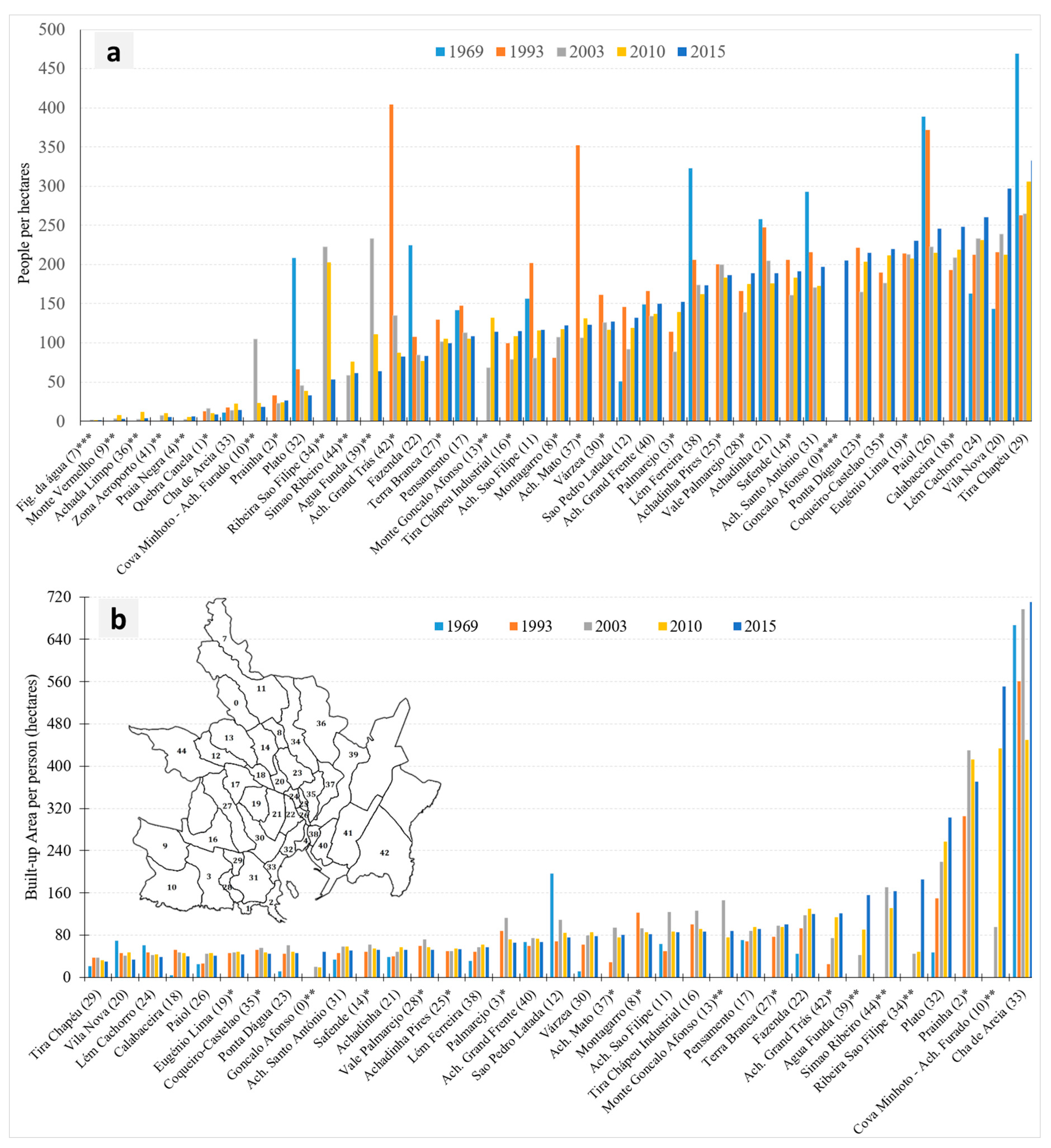
At zonal levels, the scenario varies across the period of study. For instance, older zones tended to be higher in density than recent zones, although some had a decline in population during that time. Zones like Platô (the historic center) are not a part of this trend, because it is a commercial and service zone. In 2015, Platô had only 19.9% of the 1969 population, a loss of about 3490 residents. Moreover, lower UD and higher LCR (Figure 6) occur due to a concentration of infrastructure that does not require housing (e.g., sports facilities, government institutions, commercial and industrial spaces with warehouses, military barracks). A higher UD during the period of analysis was observed for the years 1969 (Platô, Fazenda, Lém Ferreira, Achadinha, Achada Santo António, Paiol, and Tira Chapéu) and 1993 (Achada Grande Trás, Achada São Filipe, Achada Mato, Achadinha, Paiol, and Tira Chapéu).
Montagarro, Calabaceira, and Lém Cachorro have always shown an increase in UD from 1969 to 2015, unlike Platô, Cova Minhoto-Achada Furada, Ribeira São Filipe, Água Funda, and Achada Grande Trás, which have always decreased. Most of the remaining zones have shown a decline in UD.
Even though the population is strongly correlated with urban areas (Figure 5a), this relationship is not necessarily reflected for all zones in the study area. Therefore, further analysis should be done to verify that in fact the change in built-up area occurs in zones where the population has increased. Thus, in order to understand this phenomenon, we applied regression analysis, using said explanatory variables (Table 1).
3.2. Driving Forces of Urban Expansion in the Study Area
The population, age of zones, road density, distance to industrial zones, socioeconomic indicators, distance to arterial roads, neighborhood land available, neighborhood socioeconomic indicators, and distance to center have a positive relationship with urban expansion in Praia from 1993 to 2015. However, the combination of driving forces varies over time.
Table 4 shows how different factors have been driving urban expansion in different manners at different times. For instance, for 1993, only two variables, population and road density, explained 90% of variation in urban expansion; 81% was explained by population, distance from industrial zones, and road density in the year 2003; and 63% was explained by distance to arterial roads, road density, and extent of infrastructure in the year 2010. Meanwhile, distance to coast, road density, number of infrastructure, distance to urban perimeter, and industrial areas explained 65% of variation in urban expansion for the year 2015. Such variables have preserved their positive effect on the expansion of urban areas over time (Appendix B). On the other hand, variables such as distance to the coast, slope, average number of floors, extent of infrastructure, industrial zones, and distance to the urban perimeter have shown a consistent negative relationship with urban expansion.
Variables such as distance to the university, soil price, neighborhood soil price, and neighborhood extent of infrastructure were a part of some model with no defensible relationship and with a weak R2 (< 0.60). Elevation does not have a statistically significant relationship with urban expansion in our study area.
3.3. OLS Results Interpretation and Validation
Table 4 shows all the results of the selected OLS passing models for each year of analysis (1993, 2003, 2010, and 2015) and their interpretation. Passing models are those that satisfied all the OLS regression requirements, as previously discussed. The aim was to reconcile higher R2 and explanatory variables with a defensible variable relationship with urban expansion for each period of analysis.
3.4. Historic Driving Forces of Urban Expansion
For 1993, we verified a positive relationship between population and urban expansion. The results show that the denser the roads, the more built-up the areas. Other models with high adjusted R2 were selected (Appendix B) in order to appreciate how the combination of other variables helps to explain the urban expansion process in the said period. For example, the association of slope, distance to the coast, and population explains about 75% of the variation in built-up growth. Both slope and distance to the coast interact negatively with urban expansion.
For the year 2003, the model with higher adjusted R2 (0.81) contains, apart from population and road density variables, the distance from industrial zones. The population and road density variables kept their relationship with urban expansion. The distance from industrial zones variables coefficient suggested that urban expansion tends to occur further from industrial areas. Other groups of models that report satisfactory adjusted R2 (> 0.70) with a certain explanatory power and defensible relationship are shown in Appendix B. For example, model C2 suggests that an increase in socioeconomic indicators positively impacts urban expansion, when associated with the population, distance from industrial zones and mean slope variables. In all four models (i.e., C1, C2, C3, and C4), population kept its positive relationship with urban expansion. In model C3, the age of the zone also reported a positive relationship, when associated with population, distance from industrial zones, and slope—the same as model C4.
For 2010, 63% of the variability in urban expansion may be explained by only three variables (Table 4). The population is not statistically significant, although we expected the contrary. Another model with a lower R2 (Appendix B, Table A2 (D2)) shows that, besides the distance to arterial roads, road density, and neighborhood land available, the number of floors and neighborhood socioeconomic indicators influenced the trend of urban expansion in the city of Praia. Among these variables, only number of floors has a negative relationship with urban expansion. These facts will be clarified in the discussion section. For the subsequent period, 2010–2015, the distance to the coast and road density kept their positive relationship with urban expansion. By contrast, the extent of infrastructure kept its negative relationship with urban expansion, as expected (Table 4E), e.g., Água Funda, Monte Vermelho, and Terra Branca. The last three variables associated with industrial areas (dummy variables) and distance to urban perimeter together explain about 65% of the urban expansion of the city of Praia.
This is similar to the second chosen model, which shows another combination of explanatory variables, with distance to center instead of extent of infrastructure. We noticed that from 1993 to 2015, all the statistically significant explanatory variables have kept their relationship with urban expansion over time, suggesting some consistency.
4. Discussion
4.1. Urban Expansion and Comparison with Other Studies
Rapid urban expansion in the city of Praia started in 1975 after the national independence. With a succession of years of drought and the emergence of industrial clusters, people eventually moved from rural areas and other islands to the capital city [46]. Therefore, the majority of urban expansion in the study period 1969–1993 was concentrated during the interval 1975–1993. For the year 1969, the higher UD (238 people/ha) compared to the subsequent periods may justify the lower annual expansion of urban areas (12.3 ha/year) and the compact growth (Figure 3). Although we registered a decrease in UD from 1969 to 1993, the annual decrease is less than in the period 1993 to 2003 (approx. 2 people/ha vs. approx. 4 people/ha). From 1993 to 2003, this decrease in UD represents an unnecessary increase of urban area to accommodate 1472 new people, which can explain the higher urban expansion in that period. However, the absence of jobs data is a weakness of this metric.
The approval of the first law for the policy on territorial management and urbanism in 1993 (LBOTPU–Lei no. 85/IV/93) and the extensive revision of the law of soil in 2007 (DLeg. no. 2/2007) have changed the regulation and control of land use, e.g., the obligation to develop urban plans for municipality councils. In the city of Praia, the development of such plans was more significant after the year 2000, which may be associated with the decline in urban expansion from 2003 to 2015. In addition, the impact of the multi-family buildings project “Casa para todos—Housing for Everybody” started in 2010, which led to the construction of 2100 dwellings to reduce the housing deficit and pressure on the land [13].
The built-up area of Praia city increased 10-fold from 1969 to 2015, while the population increased 6-fold, indicating an increase in soil consumption. Angel et al. [22] have found the same trend in 120 cities, while Gao et al. [53] observed it in 438 small Chinese cities. The annual decrease rate in UD in the city of Praia is 0.9% versus the 1.7% reported by Angel.
Praia recorded rapid horizontal expansion. The 97 ha of built-up area in 1969 grew to 1028 ha in 2015 at an average growth rate of about 21% (20 ha/year). Literature on the urban expansion rate at the scale of this study is scant as most previous studies focused on larger cities [6]. However, Haregeweyn et al. [16] reported an annual growth rate of urban areas of 31% (88 ha/year) in Bahir Dar city, Ethiopia, for the period 1957–2009, while Gao et al. [53] reported a 10.8% growth rate in China during the period 1990–2010. Cape Verde, a small territory (4033 km2) compared to the said countries, recorded only 10% of arable land. The total urban areas of Praia in 2015 represent 11.2% of the total urban built-up area in Cape Verde (9178 ha), the latter of which was projected by Angel [5], and approximately 1% of the Santiago Island surface.
4.2. Historical Driving Forces and Comparison with Other Studies
Although the driving forces did not necessarily constantly influence urban expansion for all four periods of analysis (Table 4 and Appendix B), their effect on urban expansion was maintained over time.
Previous studies have shown population growth as a primary driving force of urban expansion [54,55]. However, our findings show that population growth did not always influence urban expansion in Praia city. The population strongly influenced urban expansion in Praia city only until 2003. Nevertheless, this relationship became weaker after that period (not statistically significant). This means that, even though the urban areas of Praia grew linearly with population (Figure 5a), such growth did not occur in the zones where we verified population growth. This fact may be associated with the desire for second homes [23]: by constructing a new house and keeping the permanent residence in the habitual zones is quite common in Praia. For example, in Cova Minhoto-Achada Furada (ID = 10 on the map), even though we registered a faster urban expansion (Figure 7), we registered lower UD, similar to Palmarejo (ID = 3).
From 1993 to 2003, zones further from industrial areas have registered more urban expansion than those close to them, and zones with industrial areas tend to have less urban expansion. Although this appears contradictory to previous studies [54,56], it may be related to locations of mostly industrial areas between zones with consolidated urban areas (e.g., Praia Negra) and zones located far from public easements (e.g., Zona Aeroporto, Achada Grande Trás, and Achada Grande Frente), which negatively affect urban expansion. Such zones are also located in urban periphery with relatively weak public transport. On the other hand, large portions of land in such zones have been reserved by the government for future port and airport expansion [13]. As mentioned previously, industrial built-up areas were removed as part of urban areas (dependent variable) in order to approximate our understanding of residential behavior.
Our findings show that, for the period 2003–2010, zones with less infrastructure and further from arterial roads registered more expansion. This fact is contradictory to Pravitasari et al. [56] but, in the present study area, this was expected because a large part of the urban expansion in Praia occurs in peripheral zones (Figure 7). This is because Praia was dominated by edge-expansion growth (Figure 4) in the said period, but also because zones closer to the arterial roads were already consolidated. These zones have a prevalence of poverty and scarcity of basic infrastructure and weak land-use controls (e.g., Água Funda, Achada Mato, Terra Branca, and Varzea) [36]. Additionally, even Cova Minhoto-Achada Furada, which is a prime zone, lacks infrastructure. The majority of Praia urban plans were more interested in producing lots of land, without ensuring the availability of basic infrastructure [13].
The higher socioeconomic indicators in the surroundings positively influence urban expansion in Praia. This means that people tend to live closer to areas that offer more opportunities for employment, urban infrastructure, and accessibility. We also observed, similar to previous studies [23], that neighborhood land availability has influenced urban expansion, showing a people’s preference for living in open spaces in Praia.
Our results suggest that the fewer floors there are in buildings, the more urban expansion is recorded. This means that low-rise buildings promote more construction and consequently horizontal expansion. In fact, vertical construction of buildings allows for an improvement in the utilization of land, with more people living in the same space, thereby preserving open and natural spaces [57,58].
Sometimes due to the irregularity of topography and coast lines, some zones seem to be close to the center if we consider the Euclidian distance. However, such zones are merely peripheral zones and not really close if we consider the road network. Therefore, it is useful to include both variables, distance to the center and distance to the urban perimeter, to reduce the subjectivity of the center effect, since they do not present multicollinearity problems.
Few studies have been conducted regarding urban expansion in SIDS, although they have been experiencing rapid urban expansion in contrast to their limited arable soil [9]. This study fills these gaps and will also be of particular interest to those who aim to use vector data to delineate urban settlements. This technique can also be applied after high-resolution image classification in order to smooth the outputs. In addition, it can be a helpful instrument for policy-makers in the urban planning process.
Most studies have used accumulative built-up area as a dependent variable in the regression models for the exploration of their driving forces [11,16], which has often shown a strong correlation between urban area and population. However, we believe that urban area for some zones cannot be a result of population, especially where we registered a decrease in population. For example, Platô was totally consolidated in 1993 (Figure 4), when it had approximately 1561 inhabitants. Therefore, it is not factual to relate such urban areas from the year 1993 with 867 inhabitants from the year 2015, assuming some relationship that does not exist. Therefore, our method allows us to better capture variations over time and better relate the built-up areas and population by considering both changes over the same period of time.
This study has its limitations. Although the technique used to obtain building footprints for the year 2015 is useful, specifically for urban scales where high spatial resolution images are a concern, it is still limited where urban areas have significant vegetation that may render it difficult to define the boundaries of the building footprints.
5. Conclusions
Based on the integration of multi-temporal data into the consistent vector dataset, we observed a rapid urban expansion in Praia during the period 1969–2015. The urban land increased by 960%, from 97 ha to 1028 ha. The majority of Praia’s built-up areas (62.8%) have emerged in the last 22 years, showing the fast urbanization process in recent decades. However, the period 1993–2003 was more dynamic (36.8 ha/year). The UD had decreased (238 people/ha to 140 people/ha), with a consequent increase in LCR (42.1 m2/person to 71.6 m2/person).
Different factors have driven the urban expansion in Praia in different periods. The population has influenced the urban expansion from 1993 to 2003. From this time until 2015, significant urban expansion did not occur in zones where we verified population growth. Therefore, population and density of roads showed a positive relationship with urban expansion and distance to the coast and slope, but a negative relationship in the period 1969–1993. Population, distance from industrial zones, density of roads, socioeconomic indicators, and age of zones positively influenced urban expansion during 1993–2003, while slope negatively influenced it. The distance to arterial roads, density of roads, neighborhood land available, and socioeconomic indicators positively influenced the urban expansion during the period 2003–2010. The infrastructure and number of floors have a negative relationship. After this period until 2015, the density of roads and distance to center had a positive effect on urban expansion. The distance to the coast, infrastructure, industrial zone, and distance from urban perimeter have also influenced urban expansion, but with a negative relationship.
Planners and policy-makers should consider the increase in land consumption in their urban plans, by qualifying the spaces for future urban expansion, promoting vertical construction, coverage for infrastructure, and improvement of accessibility in the periphery while improving the quality of life of the inhabitants. This study can provide useful data that will contribute to decision makers’ understanding of urban expansion and predictions of land area for future planning.
Acknowledgments
This study is funded by the National Natural Science Foundation of China (No. 41471325), the Scientific and Technological Leading Talent Fund of National Administration of Surveying, mapping and geo-information (2014), and the Wuhan “Yellow Crane excellence” (Science and technology) program (2014). We cordially thank Constantino Semedo from Praia Municipal Council and Euda Miranda from National Institute of Territory Management of Cape Verde for their support in data collection. We also thank Mrs. Lauren Roseinshein for her kind feedback about the OLS model.
Author Contributions
Patrik Silva and Li Lin contributed to the study design and manuscript writing. Patrik Silva designed and performed the analysis.
Conflicts of Interest
The authors declare no conflict of interest.
Appendix A. Calculation of Explanatory Variables

Table A1.
Calculation of some explanatory variables.
| Variables | Description | |
|---|---|---|
| Socioeconomics variables | Socioeconomic variables are the average of percentage of population in each zone living in the following conditions (based on our calculation): Source of water resources: Domiciliary water connection and auto-tank; Source of energy for cooking: Gas, electricity; Source of energy for illumination: Electricity (2003 and 2010) Sanitation: domiciliary connection to septic tanks or sewage system (2003); Possession of goods and services: Refrigerator, television (2003) in addition to stove, washing machine, air conditioning, automobile, telephone, computer, cable TV, Internet (2010); and level of education: High school, higher education, (2003); Comfort level: Median, high and very high (2010). We considered these variables as indicators of level of social life in each zone. | |
| Average price of soil | A shapefile that includes the delimitation of price of soil in the city of Praia, was intersected with the administrative zonal boundaries to calculate the average price of soil for each zone using the right formula: Where, ASP is the average of price of soil in zone i; SP1 is the soil price in the zone i; ASP1 is the area occupied by the soil price i; AZ is the area of the zone (or changed urban area) where ASP1 is located. | |
| Avg. number of floors | The number of floors shapefile were intersected with the administrative zones of Praia (2015) or patches grown for the year 2010 and then we summarized the average number of floors for each zone using ArcGIS. | |
| Number of infrastructure | The number of infrastructure was obtained by georeferencing and digitizing the map of infrastructure (CMP, 2014). | |
| Land available | For the calculation of land available for future urban expansion, we excluded the areas considered as not feasible for the construction of buildings. Such areas include geophysical limitations: mountains, water streams, slope steeper than 45ᴼ. | |
| Road density | The roads were classified as arterial roads, main roads, and secondary roads. Arterial roads are the highways. Main roads include arterial roads and all the roads that give access to each zone in particular. | |
| Secondary roads are roads that allow the circulation inside each zone. So, the density of roads for each zone was calculated by area weighted by type of roads (70% for main roads and 30% for secondary roads). Where, Drd is road density index, AMrd is the area (m2) of the main roads in zone i, ASrd is the area (m2) of secondary roads in the zone i and AZ is the size of zone. | ||
Appendix B. OLS Model Results
Table A2.
Other interesting models: summary.
| Summary OLS—1993 (B2) n = 32; variable = 3 | |||||
| Variable | Coefficient | Std-error | t-statistic | Robust_Pr | VIF |
| Intercept | 65,668.825059 | 18,085.944265 | 3.630932 | 0.006256 * | |
| Population | 36.541527 | 3.944321 | 9.264340 | 0.000000 * | 1.049561 |
| Distance to coast | −8.731622 | 6.129818 | −1.424450 | 0.043948 * | 1.009154 |
| Mean slope | −3185.661099 | 1808.962638 | −1.761043 | 0.023930 * | 1.053457 |
| Adjusted R2 | 0.759034 | ||||
| R2 | 0.782354 | ||||
| AICc | 777.949357 | ||||
| F-statistic | 33.549664 | Prob(>F), (3, 28) degrees of freedom: | 0.000000 * | ||
| Wald statistic | 63.931454 | Prob(>chi-squared), (3) degrees of freedom: | 0.000000 * | ||
| Koenker (BP) statistic | 8.321808 | Prob(>chi-squared), (3) degrees of freedom: | 0.039809 * | ||
| Jarque-Bera statistic | 2.419131 | Prob(>chi-squared), (2) degrees of freedom: | 0.298327 | ||
| Summary OLS—2003 (C2) n = 38; variable = 4 | |||||
| Variable | Coefficient | Std-error | t-statistic | Robust_Pr | VIF |
| Intercept | 3547.167864 | 25,570.606772 | 0.138721 | 0.810405 | |
| Population | 84.047560 | 8.371864 | 10.039288 | 0.000001 * | 1.034508 |
| Distance from industrial zone | 51.133256 | 17.881194 | 2.859611 | 0.018732 * | 1.146617 |
| Mean slope | −7786.452316 | 2664.749176 | −2.922021 | 0.004443 * | 1.131716 |
| Socioeconomic factors | 9851.451136 | 4694.156520 | 2.098663 | 0.005870 * | 1.058790 |
| Adjusted R2 | 0.777430 | ||||
| R2 | 0.801492 | ||||
| AICc | 945.164522 | ||||
| F-statistic | 33.309981 | Prob(>F), (4, 33) degrees of freedom: | 0.000000 * | ||
| Wald statistic | 51.611040 | Prob(>chi-squared), (4) degrees of freedom: | 0.000000 * | ||
| Koenker (BP) statistic | 16.308520 | Prob(>chi-squared), (4) degrees of freedom: | 0.002632 * | ||
| Jarque-Bera statistic | 0.211597 | Prob(>chi-squared), (2) degrees of freedom: | 0.899606 | ||
| Summary OLS—2003 (C3) n = 38; variable = 4 | |||||
| Variable | Coefficient | Std-error | t-statistic | Robust_Pr | VIF |
| Intercept | 12,879.160852 | 23,960.185097 | 0.537523 | 0.410583 | |
| Population | 88.365231 | 8.423218 | 10.490674 | 0.000001 * | 1.031689 |
| Age of Zone | 568.907423 | 289.978593 | 1.961895 | 0.001423 * | 1.131379 |
| Distance from industrial zone | 53.393931 | 18.336335 | 2.911919 | 0.011392 * | 1.187829 |
| Mean slope | −8310.379996 | 2737.885508 | −3.035328 | 0.003002 * | 1.176952 |
| Adjusted R2 | 0.774076 | ||||
| R2 | 0.798500 | ||||
| AICc | 945.732950 | ||||
| F-statistic | 32.692927 | Prob(>F), (4, 33) degrees of freedom: | 0.000000 * | ||
| Wald statistic | 53.192196 | Prob(>chi-squared), (4) degrees of freedom: | 0.000000 * | ||
| Koenker (BP) statistic | 17.325807 | Prob(>chi-squared), (4) degrees of freedom: | 0.001671 * | ||
| Jarque-Bera statistic | 0.526457 | Prob(>chi-squared), (2) degrees of freedom: | 0.768566 | ||
| Summary OL—2003 (C4) n = 38; variable = 3 | |||||
| Variable | Coefficient | Std-error | t-statistic | Robust_Pr | VIF |
| Intercept | 37,457.392394 | 24,768.187780 | 1.512319 | 0.061513 | |
| Population | 89.306533 | 9.296813 | 9.606145 | 0.000001 * | 1.030170 |
| Age of zone | 341.587770 | 308.464408 | 1.107381 | 0.032554 * | 1.049383 |
| Mean slope | −5556.040099 | 2837.863428 | −1.957825 | 0.033879 * | 1.036475 |
| Adjusted R2 | 0.724377 | ||||
| R2 | 0.746725 | ||||
| AICc | 951.588354 | ||||
| F-statistic | 33.413816 | Prob(>F), (3, 34) degrees of freedom: | 0.000000 * | ||
| Wald statistic | 41.233657 | Prob(>chi-squared), (3) degrees of freedom: | 0.000000 * | ||
| Koenker (BP) statistic | 13.505063 | Prob(>chi-squared), (3) degrees of freedom: | 0.003662 * | ||
| Jarque-Bera statistic | 3.505962 | Prob(>chi-squared), (2) degrees of freedom: | 0.173257 | ||
| Summary OLS—2003 (C5) n = 38; variable = 2 | |||||
| Variable | Coefficient | Std-error | t-statistic | Robust_Pr | VIF |
| Intercept | −16,641.976141 | 13,128.577735 | −1.267615 | 0.136854 | |
| Population | 77.976537 | 8.602076 | 9.064851 | 0.000000 * | 1.141424 |
| Road density | 14,753.736779 | 3.848730 | 3.848730 | 0.006231 * | 1.141424 |
| Adjusted R2 | 0.787032 | ||||
| R2 | 0.798543 | ||||
| AICc | 940.227212 | ||||
| F-statistic | 69.367333 | Prob(>F), (2, 35) degrees of freedom: | 0.000000 * | ||
| Wald statistic | 69.817332 | Prob(>chi-squared), (2) degrees of freedom: | 0.000000 * | ||
| Koenker (BP) statistic | 10.162278 | Prob(>chi-squared), (2) degrees of freedom: | 0.006213 * | ||
| Jarque-Bera statistic | 1.541636 | Prob(>chi-squared), (2) degrees of freedom: | 0.462635 | ||
| Summary OLS—2003 (C6) n = 38; variable = 2 | |||||
| Variable | Coefficient | Std-error | t-statistic | Robust_Pr | VIF |
| Intercept | 46,550.009155 | 23,443.004139 | 1.985667 | 0.042692 * | |
| Population | 87.899806 | 9.239340 | 9.513645 | 0.000001 * | 1.010936 |
| Mean slope | −5062.737893 | 2811.728063 | −1.800579 | 0.047269 * | 1.010936 |
| Adjusted R2 | 0.722595 | ||||
| R2 | 0.737590 | ||||
| AICc | 950.271901 | ||||
| F-statistic | 49.189541 | Prob(>F), (2,35) degrees of freedom: | 0.000000 * | ||
| Wald statistic | 38.190853 | Prob(>chi-squared), (2) degrees of freedom: | 0.000000 * | ||
| Koenker (BP) statistic | 11.661848 | Prob(>chi-squared), (2) degrees of freedom: | 0.002935 * | ||
| Jarque-Bera statistic | 3.748749 | Prob(>chi-squared), (2) degrees of freedom: | 0.153451 | ||
| Summary OLS—2010 (D2) n = 41; variable = 5 | |||||
| Variable | Coefficient | Std-error | t-statistic | Robust_Pr | VIF |
| Intercept | −126,652.313013 | 37,469.726328 | −3.380124 | 0.020394 * | |
| Distance to arterial roads | 74.617275 | 17.078503 | 4.369076 | 0.001547 * | 1.180858 |
| Road density | 14,318.952809 | 3392.340391 | 4.220966 | 0.001602 * | 2.658833 |
| Average number of floors | −34,505.961914 | 15,665.314281 | −2.202698 | 0.010020 * | 2.882851 |
| Neighb. land available | 0.065042 | 0.019144 | 3.397443 | 0.002504 * | 2.053562 |
| Neig. avg socioecon. indicat. | 162.742782 | 42.136419 | 3.862283 | 0.006788 * | 2.165538 |
| Adjusted R2 | 0.608417 | ||||
| R2 | 0.657365 | ||||
| AICc | 58.684142 | ||||
| F-statistic | 13.429898 | Prob(>F), (5, 35) degrees of freedom: | 0.000000 * | ||
| Wald statistic | 23.205349 | Prob(>chi-squared), (5) degrees of freedom: | 0.000308 * | ||
| Koenker (BP) statistic | 24.291281 | Prob(>chi-squared), (5) degrees of freedom: | 0.000191 * | ||
| Jarque-Bera statistic | 3.896771 | Prob(>chi-squared), (2) degrees of freedom: | 0.142504 | ||
| Summary OLS—2015 (E2) n = 41; variable = 5 | |||||
| Variable | Coefficient | Std-error | t-statistic | Robust_Pr | VIF |
| Intercept | 65,621.443897 | 13,909.629218 | 4.717699 | 0.000053 * | |
| Distance to left | 14.197743 | 4.196104 | 3.383553 | 0.000543 * | 2.561907 |
| Distance to coast | −22.743622 | 4.950717 | −4.594006 | 0.000317 * | 4.923847 |
| Road density | 4894.662978 | 1229.073300 | 3.982401 | 0.006499 * | 1.254978 |
| Industrial area (binary variable) | −31846.651186 | 9884.405562 | −3.221909 | 0.000304 * | 1.506324 |
| Distance to urban perimeter | −43.593186 | 7.053607 | −6.180269 | 0.000003 * | 2.970793 |
| Adjusted R2 | 0.653254 | ||||
| R2 | 0.696597 | ||||
| AICc | 931.732624 | ||||
| F-statistic | 23.879429 | Prob(>F), (5, 35) degrees of freedom: | 0.000000 * | ||
| Wald statistic | 25.943000 | Prob(>chi-squared), (5) degrees of freedom: | 0.000000 * | ||
| Koenker (BP) statistic | 16.152417 | Prob(>chi-squared), (5) degrees of freedom: | 0.002063 * | ||
| Jarque-Bera statistic | 1.836169 | Prob(>chi-squared), (2) degrees of freedom: | 0.424394 | ||
* Statistically significant at 0.05 level.
References
- Angel, S. The NYU Urban Expansion Program: A Primer. Available online: http://marroninstitute.nyu.edu/uploads/content/UEPrimer2015.pdf (accessed on 8 August 2017).
- Brockerhoff, M.P. An Urbanizing World; Population Reference Bureau: Washington, DC, USA, 2000. [Google Scholar]
- UNFPA. State of World Population 2007: Unleashing the Potential of Urban Growth; UNFPA: New York, NY, USA, 2007. [Google Scholar]
- Jaeger, J.A.G.; Bertiller, R.; Schwick, C.; Kienast, F. Suitability criteria for measures of urban sprawl. Ecol. Indic. 2010, 10, 397–406. [Google Scholar] [CrossRef]
- Angel, S.; Parent, J.; Civco, D.L.; Blei, A.M. Atlas of Urban Expansion; Lincoln Institute of Land Policy: Cambridge, MA, USA, 2012. [Google Scholar]
- Nazarnia, N.; Schwick, C.; Jaeger, J.A.G. Accelerated urban sprawl in Montreal, Quebec City, and Zurich: Investigating the differences using time series 1951–2011. Ecol. Indic. 2016, 60, 1229–1251. [Google Scholar] [CrossRef]
- Bhatta, B. Analysis of Urban Growth and Sprawl from Remote Sensing Data (Advances in Geographic Information Science); Springer: Berlin, Germany, 2010. [Google Scholar]
- UN-Habitat. Urban Planning for City Leaders; UN-Habitat: Nairobi, Kenya, 2013. [Google Scholar]
- UN-Habitat. Urbanization and Climate Change in Small Island Developing States; UN-Habitat: Nairobi, Kenya, 2015. [Google Scholar]
- UN-OHRLLS. Small Islands Developing States:Small Islands Big(ger) Stakes; UN-OHRLLS: New York, NY, USA, 2011. [Google Scholar]
- Angel, S.; Parent, J.; Civco, D.L.; Blei, A.M.; Potere, D. A Planet of Cities: Urban Land Cover Estimates and Projections for All Countries, 2000–2050; Lincoln Institute of Land Policy: Cambridge, MA, USA, 2010. [Google Scholar]
- UN-OHRLLS. Small Island Developing States (SIDS) Statistics; UN-OHRLLS: New York, NY, USA, 2012. [Google Scholar]
- Câmara Municipal da Praia (CMP). Proposta do Plano Director Municipal (Proposal of the Municipal Master Plan); CMP: Praia, Cape Verde, 2014. [Google Scholar]
- Instituto Nacional de Gestão do Território (INGT). Esquema Regional do Ordenamento do Território de Santiago (Regional Scheme of Territorial Planning for Santiago island); INGT: Praia, Cape Verde, 2010. [Google Scholar]
- Li, X.; Zhou, W.; Ouyang, Z. Forty years of urban expansion in Beijing: What is the relative importance of physical, socioeconomic, and neighborhood factors? Appl. Geogr. 2013, 38, 1–10. [Google Scholar] [CrossRef]
- Haregeweyn, N.; Fikadu, G.; Tsunekawa, A.; Tsubo, M.; Meshesha, D.T. The dynamics of urban expansion and its impacts on land use/land cover change and small-scale farmers living near the urban fringe: A case study of Bahir Dar, Ethiopia. Landsc. Urban Plan. 2012, 106, 149–157. [Google Scholar] [CrossRef]
- Dubovyk, O.; Sliuzas, R.; Flacke, J. Spatio-temporal modelling of informal settlement development in Sancaktepe district, Istanbul, Turkey. ISPRS J. Photogramm. Remote Sens. 2011, 66, 235–246. [Google Scholar] [CrossRef]
- Braimoh, A.K.; Onishi, T. Spatial determinants of urban land use change in Lagos, Nigeria. Land Use Policy 2007, 24, 502–515. [Google Scholar] [CrossRef]
- Chen, J.; Chang, K.; Karacsonyi, D.; Zhang, X. Comparing urban land expansion and its driving factors in Shenzhen. Habitat Int. 2014, 43, 61–71. [Google Scholar] [CrossRef]
- Lu, C.; Wu, Y.; Shen, Q.; Wang, H. Driving force of urban growth and regional planning: A case study of China’s Guangdong Province. Habitat Int. 2013, 40, 35–41. [Google Scholar] [CrossRef]
- Weilenmann, B.; Seidl, I.; Schulz, T. The socio-economic determinants of urban sprawl between 1980 and 2010 in Switzerland. Landsc. Urban Plan. 2017, 157, 468–482. [Google Scholar] [CrossRef]
- Angel, S.; Sheppard, S.C.; Civco, D.L.; Buckley, R.; Chabaeva, A.; Gitlin, L.; Kraley, A.; Parent, J.; Perlin, M. The Dynamics of Global Urban Expansion; World Bank: Washington, DC, USA, 2005. [Google Scholar]
- Ewing, R. Is Los Angeles-style sprawl desirable? J. Am. Plan. Assoc. 1997, 63, 107–126. [Google Scholar] [CrossRef]
- Taubenböck, H.; Esch, T. Remote Sensing—An Effective Data Source for Urban Monitoring. 2011. Available online: https://earthzine.org/2011/07/20/remote-sensing-an-effective-data-source-for-urban-monitoring/ (accessed on 23 December 2016).
- Deng, X.; Huang, J.; Rozelle, S.; Uchida, E. Growth, population and industrialization, and urban land expansion of China. J. Urban Econ. 2008, 63, 96–115. [Google Scholar] [CrossRef]
- Kuang, W.; Liu, J.; Dong, J.; Chi, W.; Zhang, C. The rapid and massive urban and industrial land expansions in China between 1990 and 2010: A CLUD-based analysis of their trajectories, patterns, and drivers. Landsc. Urban Plan. 2016, 145, 21–33. [Google Scholar] [CrossRef]
- Ferreira, J.A.; Condessa, B.; Castro, J.; Pinto, P. Urban settlements delimitation in low-density areas—An application to the municipality of Tomar (Portugal). Landsc. Urban Plan. 2010, 97, 156–167. [Google Scholar] [CrossRef]
- Turker, M.; Koc-san, D. Building extraction from high-resolution optical spaceborne images using the integration of support vector machine (SVM) classification, Hough transformation and perceptual grouping. Int. J. Appl. Earth Obs. Geoinf. 2015, 34, 58–69. [Google Scholar] [CrossRef]
- Harig, O.; Burghardt, D.; Hecht, R. A Supervised Approach to Delineate Built-Up Areas for Monitoring and Analysis of Settlements. Int. J. Geo-Inf. 2016, 5, 137. [Google Scholar] [CrossRef]
- Millward, H. A vector GIS extension for generalization of binary polygon patterns. Cartogr. Int. J. Geogr. Inf. Geovis. 2004, 39, 55–64. [Google Scholar] [CrossRef]
- Zhou, Q. Comparative Study of Approaches to Delineating Built-Up Areas Using Road Network Data. Trans. GIS 2015. [Google Scholar] [CrossRef]
- Carvalho, J.; Pais, C. A Ocupação Dispersa, à escala local, nas Cidades de Aveiro-Ílhavo e Évora: identificação e caracterização (The dispersed occupation at the local level, in the cities of Aveiro-Ílhavo and Évora: Identification and characterisation) in Portuguese. In Proceedings of the Seventh International Conference on Virtual Cities and Territories (7VCT), Lisbon, Portugal, 11–13 October 2011. [Google Scholar]
- Silva, F.B.; Marques, T.S.; Delgado, C. Processos de expansão urbana e mudanças na paisagem: Ensaio metodológico (1950–2000) (Urban expansion process and change in the landscape: Methodological essay (1950–2000). In Revista da Faculdade de Letras—Geografia; Universidade do Porto: Porto, Portugal, 2012; pp. 161–183. [Google Scholar]
- Jaeger, J.A.G.; Bertiller, R.; Schwick, C.; Cavens, D.; Kienast, F. Urban permeation of landscapes and sprawl per capita: New measures of urban sprawl. Ecol. Indic. 2010, 10, 427–441. [Google Scholar] [CrossRef]
- Muhs, S.; Herold, H.; Meinel, G.; Burghardt, D.; Kretschmer, O. Computers, Environment and Urban Systems Automatic delineation of built-up area at urban block level from topographic maps. CEUS 2016, 58, 71–84. [Google Scholar] [CrossRef]
- Tavares, C. A Política de Solo na Política Urbana: A sua Relevância na Cidade Da Praia—Cabo Verde (The Urban Soil Policy: Its Relevance in the City of Praia—Cape Verde); Universidade Nova de Lisboa: Lisbon, Portugal, 2007. [Google Scholar]
- Instituto Nacional de Estatistica de Cabo Verde (INE-CV). Evolução da População Residente Urbana por Ilha e Concelho, Segundo os Censos de 1990–2010 (Evolution of the Urban Resident Population by Island and County, According to Censuses from 1990–2010); INE-CV: Praia, Cape Verde, 2010. [Google Scholar]
- Instituto Nacional de Estatistica de Cabo Verde (INE-CV). Produto Interno Bruto (PIB) por Ilha Série 2007–2012 (Gross Domestic Product (GDP) by Island, Series 2007–2012); INE-CV: Praia, Cape Verde, 2015. [Google Scholar]
- Monteiro, S.; Veiga, É.; Fernandes, É.; Fernandes, H.; Rodrigues, J.; Cunha, L. Crescimento urbano espontâneo e riscos naturais na cidade da Praia (Cabo Verde)(Spontaneous urban growth and naturals hazards in the city of Praia—Cape Verde). Cad. Geogr. 2011, 31, 117–130. [Google Scholar]
- El-Shayal, M.E.-S. First Arabian GIS software: A GIS, GPS, Database, Internet GIS software. In Proceedings of the International Symposium on Geoinformatics for Spatial Infrastructure Development in Earth and Allied Sciences (GIS-IDEAS), Ho Chi Minh City (HCMC), Vietnam, 9–11 November 2006. [Google Scholar]
- Câmara Municipal da Praia (CMP). Que Altera os Preços de Alienação de Terrenos Municipais e Fixa a Fórmula de Cálculo de Ampliações e Mudanças de Uso (Amending the Sale of Municipal Land Price and the Fixed Magnifications of Calculation Formula and Land Use Change); Imprensa Nacional de Cabo Verde: Praia, Cape Verde, 2013; p. 17. [Google Scholar]
- United Nations. Methods of Estimating Total Population for Current Dates Methods of Estimating Total Population for Current Dates; United Nations: New York, NY, USA, 1952. [Google Scholar]
- Jaeger, J.A.G.; Schwick, C. Improving the measurement of urban sprawl: Weighted Urban Proliferation (WUP) and its application to Switzerland. Ecol. Indic. 2014, 38, 294–308. [Google Scholar] [CrossRef]
- Wu, Y.; Li, S.; Yu, S. Monitoring urban expansion and its effects on land use and land cover changes in Guangzhou city, China. Environ. Monit. Assess. 2016. [Google Scholar] [CrossRef] [PubMed]
- Carneiro, L. Acerca do Crescimento Urbano no Terceiro Mundo: o caso de Cabo Verde visto através da Praia (About Urban Growth in the Third World: the case of Cape Verde seen through the Praia). Garcia da Orta Série Geogr. 1996, 15, 35–64. [Google Scholar]
- Nascimento, J.M. La Croissante et le Systeme de Gestion et de Planification de la Ville de Praia, Rep. du Cap-Vert (Growth of the system of management and planning of the city of Praia, Cape Verde republic). Ph.D. Thesis, Université de Rouen, Rouen, France, 2009. [Google Scholar]
- Haque, U.; Scott, L.M.; Hashizume, M.; Fisher, E.; Haque, R.; Yamamoto, T.; Glass, G.E. Modelling malaria treatment practices in Bangladesh using spatial statistics. Malar. J. 2012. [Google Scholar] [CrossRef] [PubMed] [Green Version]
- Poole, M.A.; Farrell, P.N.O.; Poole, A.; Farrell, N.O. The assumptions of the linear model regression. Trans. Inst. Br. Geogr. 1971, 52, 145–158. [Google Scholar] [CrossRef]
- Brunsdon, C.; Fotheringham, A.S.; Charlton, M.E. Geographically Weighted Regression: A Method for Exploring Spatial Nonstationarity. Geogr. Anal. 1996, 28, 281–298. [Google Scholar] [CrossRef]
- Scott, L.; Pratt, M. Answering Why Questions: An Introduction to Using Regression Analysis with Spatial Data. Available online: http://www.esri.com/news/arcuser/0309/files/why.pdf (accessed on 10 February 2017).
- Esri Interpreting OLS Results. Available online: http://desktop.arcgis.com/en/arcmap/10.3/tools/spatial-statistics-toolbox/interpreting-ols-results.htm (accessed on 4 November 2016).
- Rosenshein, L.; Scott, L.; Pratt, M. Finding a Meaningful Model This Checklist Will Help You Evaluate Regression Models. Available online: http://www.esri.com/news/arcuser/0111/files/findmodel.pdf (accessed on 13 March 2017).
- Gao, B.; Huang, Q.; He, C.; Sun, Z.; Zhang, D. How does sprawl differ across cities in China? A multi-scale investigation using nighttime light and census data. Landsc. Urban Plan. 2016, 148, 89–98. [Google Scholar] [CrossRef]
- Hu, Z.; Du, P.; Guo, D. Analysis of Urban Expansion and Driving Forces in Xuzhou City Based on Remote Sensing. J. China Univ. Min. Technol. 2007, 17, 267–271. [Google Scholar] [CrossRef]
- Seto, K.C.; Fragkias, M.; Güneralp, B.; Reilly, M.K. A Meta-Analysis of Global Urban Land Expansion. PLoS ONE 2011, 6, e23777. [Google Scholar] [CrossRef] [PubMed]
- Pravitasari, A.E.; Saizen, I.; Tsutsumida, N.; Rustiadi, E.; Pribadi, D.O. Local Spatially Dependent Driving Forces of Urban Expansion in an Emerging Asian Megacity: The Case of Greater Jakarta (Jabodetabek). J. Sustain. Dev. 2015, 8, 108–119. [Google Scholar] [CrossRef]
- Ali, M.M.; Al-Kodmany, K. Tall Buildings and Urban Habitat of the 21st Century: A Global Perspective. Buildings 2012, 2, 384–423. [Google Scholar] [CrossRef]
- Pank, W.; Girardet, H.; Cox, G. Tall buildings and sustainability; Corporation of London: London, UK, 2002. [Google Scholar]
Figure 1.
Study area location.
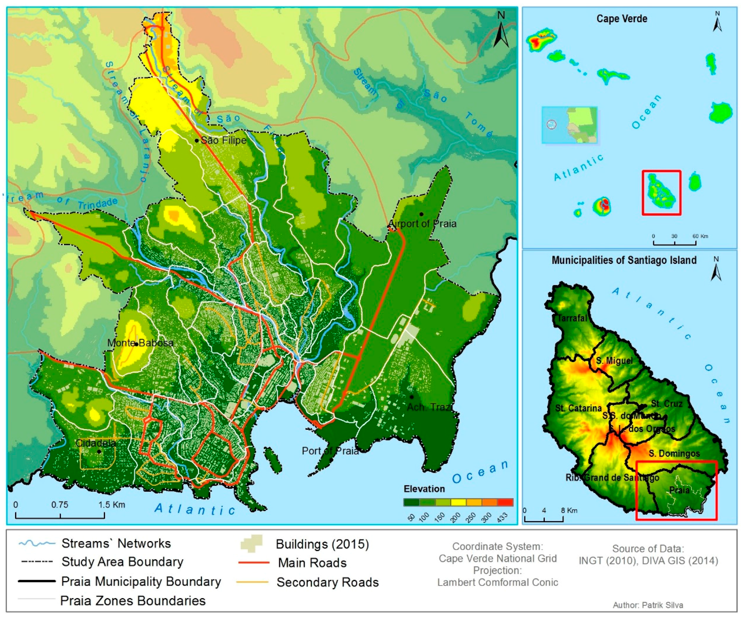
Figure 2.
Flowchart of the research methodology: (a) data preparation; (b) mapping urban expansion; and (c) exploring the driving forces of urban expansion.
Figure 2.
Flowchart of the research methodology: (a) data preparation; (b) mapping urban expansion; and (c) exploring the driving forces of urban expansion.
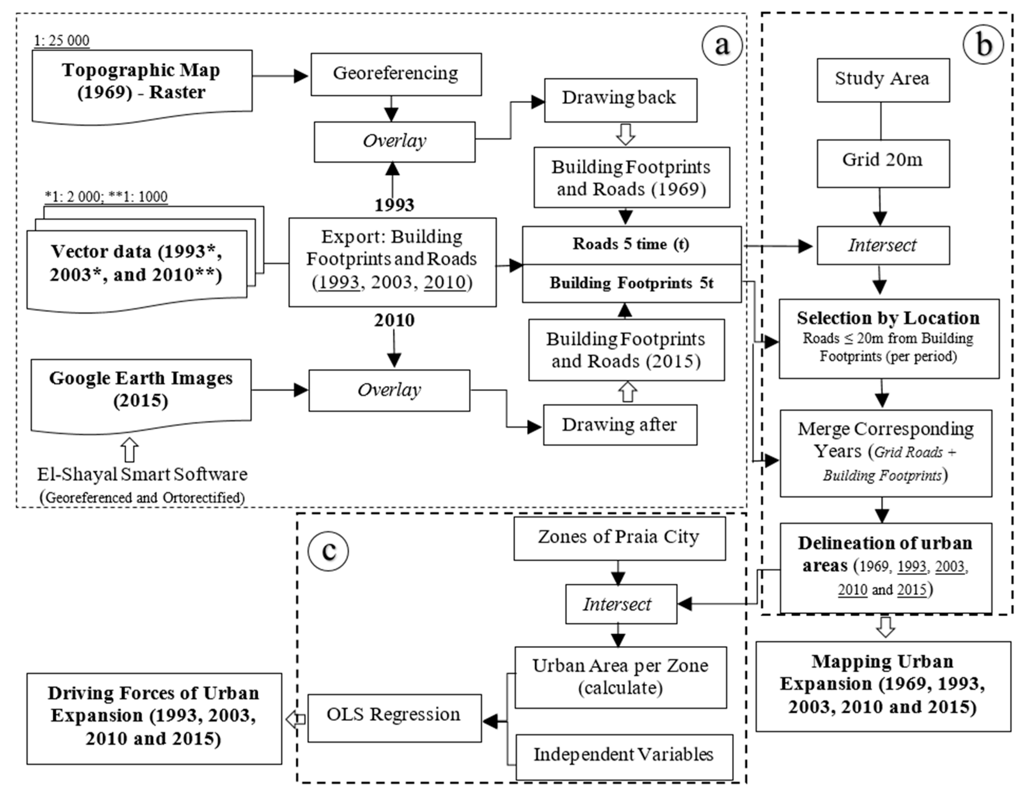
Figure 3.
Delineation of built-up areas: (a) selected roads as a part of urban areas in pink, roads within 20 m of building footprints; rejected roads as a part of urban areas in black, roads more than 20 m from building footprints; (b) outputs of urban areas delineation (both the yellow and the red areas are considered as built-up areas).
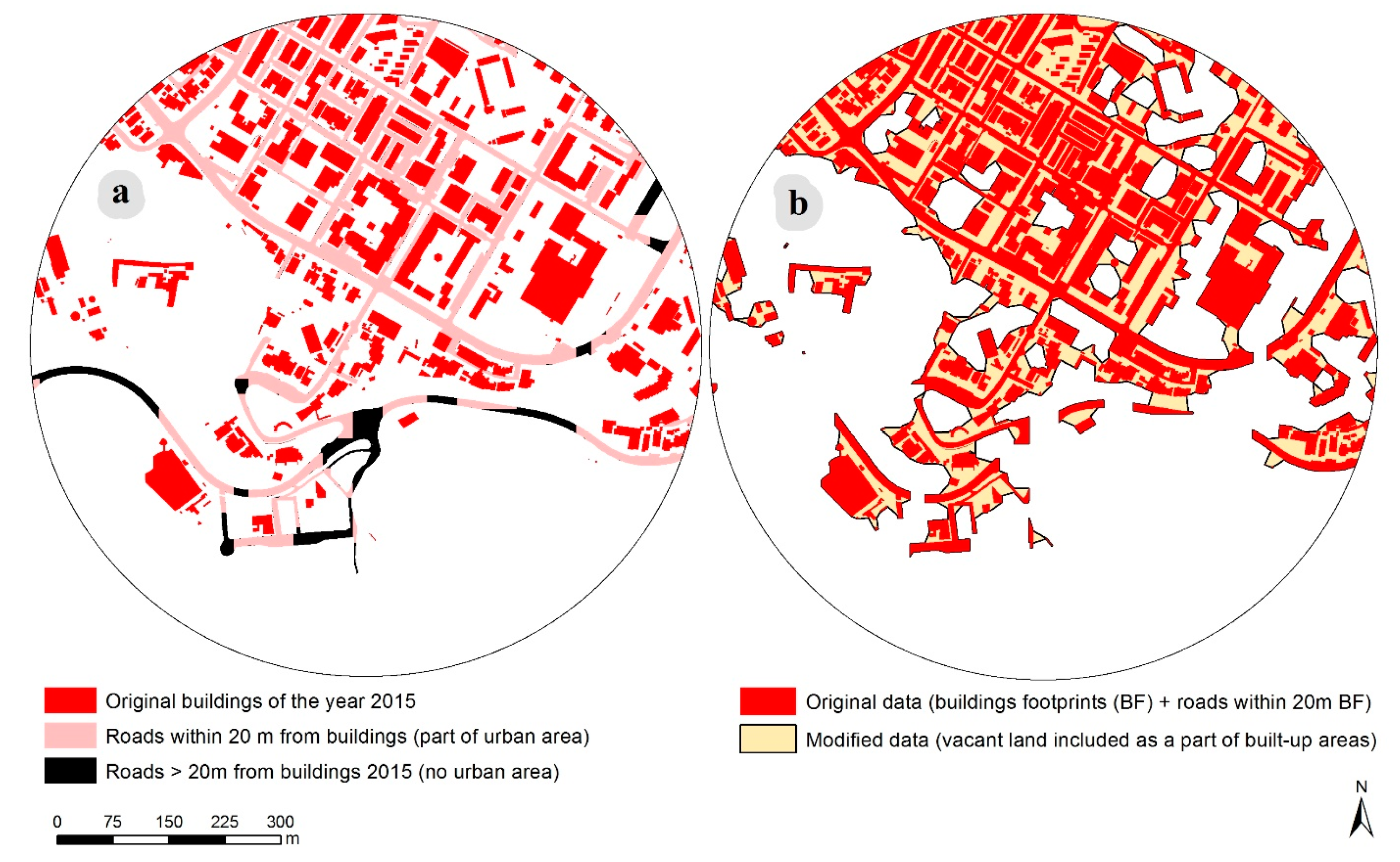
Figure 4.
Built-up areas expansion at five points in time at the city of Praia: 1969, 1993, 2003, 2010, and 2015 (source: built-up areas in 1993, 2003, 2010: planimetric data—vector datasets (INGT), built-up areas in 1969: own digitization based on national topographic maps at the scale 1:25,000 (INGT), built-up areas in 2015, own digitization based in Google Earth images obtained from El-Shayal Smart software (Smart GIS, Cairo, Egypt).
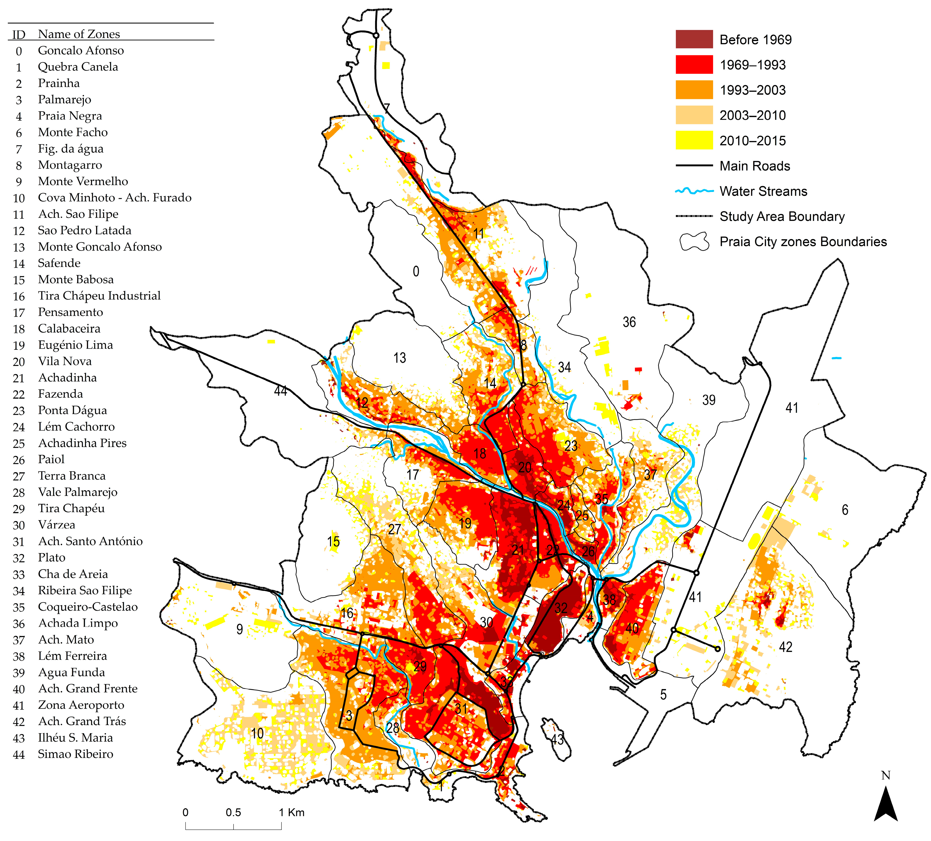
Figure 5.
(a) The relationship between built-up areas and population (Pop.) during a 46-year period in the city of Praia, from 1969 to 2015 (including industrial areas); (b) annual growth rate of built-up areas and population in the city of Praia for 1969–1993, 1993–2003, 2003–2010, and 2010–2015.
Figure 5.
(a) The relationship between built-up areas and population (Pop.) during a 46-year period in the city of Praia, from 1969 to 2015 (including industrial areas); (b) annual growth rate of built-up areas and population in the city of Praia for 1969–1993, 1993–2003, 2003–2010, and 2010–2015.
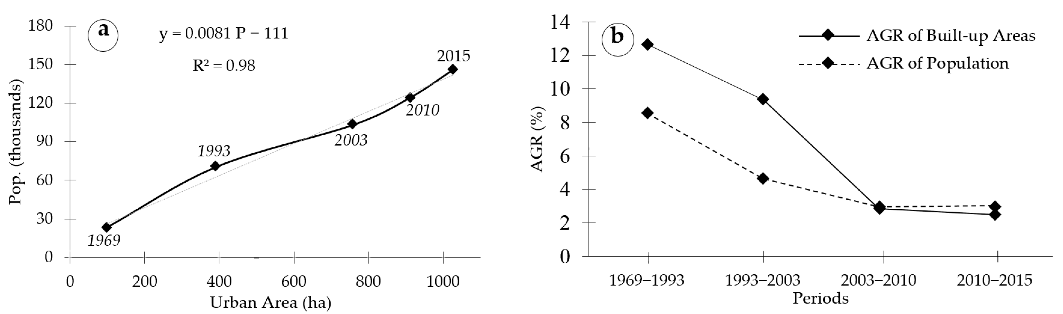
Figure 6.
(a) Population per hectares of built-up areas (UD) at zonal levels at five points in time from 1969 to 2015; (b) urban areas per person (LCR) in the city of Praia at zonal levels at five points in time from 1969 to 2015.* indicates missing data in one time step, and **** indicates missing data in four time steps, respectively.

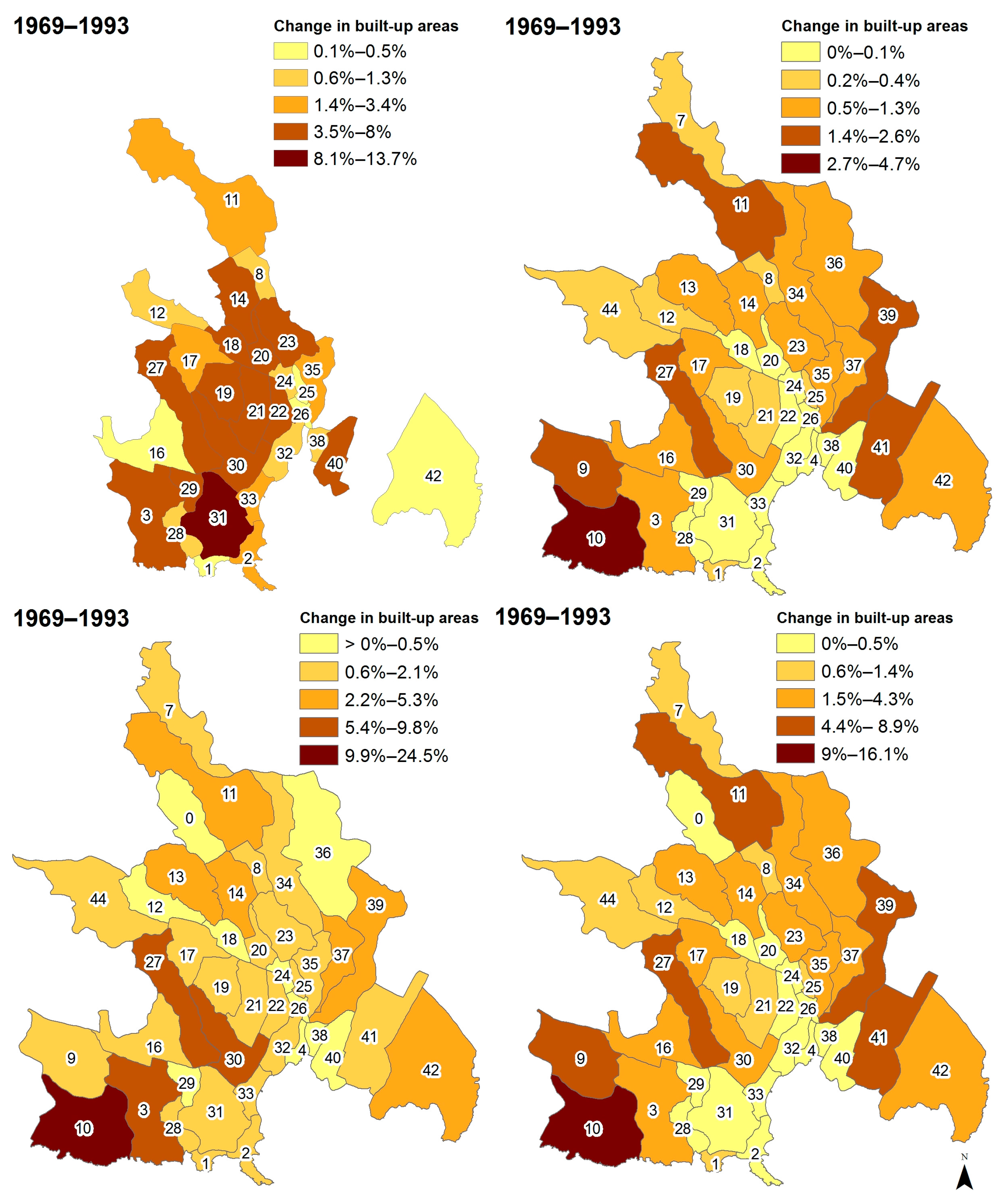
Figure 7.
Percentage of change in the built-up area in each zone relative to the total change of built-up area in the city of Praia in time i in four periods (1969–1993, 1993–2003, 2003–2010 and 2010–2015).
Figure 7.
Percentage of change in the built-up area in each zone relative to the total change of built-up area in the city of Praia in time i in four periods (1969–1993, 1993–2003, 2003–2010 and 2010–2015).

Table 1.
Candidate explanatory variables used in the OLS model.
| Variables | 1993 | 2003 | 2010 | 2015 | Description |
|---|---|---|---|---|---|
| Population | x | x | x | x | The absolute difference between the population for each zone from time i to time i − 1. |
| Road density | x | x | x | x | Area of zonal roads per total area of zone (Appendix A). |
| Age of zones | x | x | x | x | The difference in year between the year of analysis and the estimated date that the zone emerged +. |
| Distance to center | x | x | x | x | Euclidian distance between the centroid of changed urban areas for each zone in time i and the centroid to the historic center (Platô). |
| Distance to coast | x | x | x | x | Euclidian distance between the centroid of changed urban areas for each zone in time i and the coastal line. |
| Distance to arterial road | x | x | x | x | Euclidian distance between the centroid of changed urban areas for each zone in time i and the arterial road (arterial roads do not include roads that give access for the zones). |
| Distance to industrial zones | x | x | x | x | Euclidean distance between the centroid of changed urban patches to the closest industrial zone. |
| Distance to urban perimeter | x | x | Euclidean distance between the centroid of changed urban patches to the urban perimeter boundary for the interior. | ||
| Distance to university | x | x | Euclidian distance between the centroid of changed urban patches for each zone in time i and the closest university. | ||
| Mean elevation | x | x | x | x | Mean elevation of the changed urban patches for each zone in time i. |
| Mean slope | x | x | x | x | Mean slope of the changed urban patches for each zone in time i. |
| Socioeconomic variables | x | x | x | Number of people in percentage that live in each zone with indicators that show high quality of life ++. | |
| Price of soil | x | x | Average price of soil per changed urban patches in each zone in 2010; and per zone for the year 2015 +++ (Appendix A). | ||
| Average nbr of floors | x | x | Average of number of floors per changed urban patches in each zone in 2010, and per zone for the year 2015 ++++ (Appendix A). | ||
| Number of infrastructure | x | x | Number of the main public infrastructure that require daily commuting and security to the population (schools, universities, police station, main states institutions, hospitals and health centers). | ||
| Industrial zone | x | x | x | x | Dummy variable (0, 1), 1 for zones that have industrial areas, 0 otherwise. |
| Land available | x | x | x | x | The amount of land available in hectares for urban expansion. Geophysical barriers were removed from areas where we have no built-up areas in each zone (Appendix A). |
| Neighb. land available | x | x | Average of land available in neighboring zones, in hectares. | ||
| Neighb. average Socioecon. Indic. | x | x | Average of socioeconomic factors in neighboring zones, in percentage. (See Appendix A) | ||
| Neighb. number of infrastructure | x | x | Average number of infrastructure in neighboring zones. (See Appendix A) | ||
| Neighb. average price of soil | x | x | Average of soil price in neighboring zones, in Cape Verdean escudos (ECV). | ||
| OBS: The year 1969 was not considered in the OLS because the number of observations is insufficient (<30) and it does not meet the autocorrelation test assumptions. | |||||
Source: + Historical maps were obtained from National Library of Portugal; ++ Data from INE-CV—2000 and 2010 census. Data from 2000 census was used for the year 2003; +++ Product from CMP [41]; ++++ The same 2010 data used in the delineation of urban areas, with information of number of floor in each single building footprints.
Table 2.
Dynamic of urban expansion in the city of Praia (1969, 1993, 2003, 2010 and 2015).
| Periods | Range (years) | Changed UA (ha) | Pop. Growth (persons) | Annual UA Growth (ha) | Annual pop. Growth (persons) | Rate of Change in UA (%) | Rate of Change in Pop. (%) |
|---|---|---|---|---|---|---|---|
| 1969–1993 | 24 | 295 | 47,368 | 12.3 | 1974 | 304.1 | 205.2 |
| 1993–2003 | 10 | 368 | 32,751 | 36.8 | 3275 | 93.8 | 46.5 |
| 2003–2010 | 7 | 153 | 21,525 | 21.8 | 3075 | 20.1 | 20.9 |
| 2010–2015 | 5 | 114 | 18,866 | 22.9 | 3773 | 12.5 | 15.1 |
Table 3.
The relationship between urban area and population in the study area over time (1969, 1993, 2003, 2010 and 2015): urban area per person and population per unit of urban area (hectare).
Table 3.
The relationship between urban area and population in the study area over time (1969, 1993, 2003, 2010 and 2015): urban area per person and population per unit of urban area (hectare).
| Years | Urban Area (ha) | Population (persons) | Urban Area per Person (m2) | Person per Unit of Urban Area (ha) |
|---|---|---|---|---|
| 1969 | 97 | 23,082 | 42.1 | 238 |
| 1993 | 392 | 70,450 | 55.7 | 180 |
| 2003 | 760 | 103,201 | 73.7 | 136 |
| 2010 | 913 | 124,726 | 73.2 | 137 |
| 2015 | 1028 | 143,592 | 71.6 | 140 |
Table 4.
Higher adjusted R2 OLS passing models outputs at five points in time (1969, 1993, 2003, 2010 and 2015).
Table 4.
Higher adjusted R2 OLS passing models outputs at five points in time (1969, 1993, 2003, 2010 and 2015).
| Summary OLS—1993 (B) n = 32; variable = 2 | |||||
| Variable | Coefficient | Std-error | t-statistic | Probability | VIF |
| Intercept | 3985.820589 | 6785.842575 | 0.587373 | 0.561498 | |
| Population | 31.809366 | 2.517843 | 12.633579 | 0.000000 * | 1.108274 |
| Road density | 12,100.056800 | 7.480310 | 7.480310 | 0.009483 * | 1.108274 |
| Adjusted R2 | 0.907012 | ||||
| R2 | 0.913011 | ||||
| AICc | 745.776307 | ||||
| F-statistic | 152.187464 | Prob(>F), (2, 29) degrees of freedom: | 0.000000 * | ||
| Wald statistic | 518.634477 | Prob(>chi-squared), (2) degrees of freedom: | 0.000000 * | ||
| Koenker (BP) statistic | 2.417524 | Prob(>chi-squared), (2) degrees of freedom: | 0.298567 | ||
| Jarque–Bera statistic | 0.303049 | Prob(>chi-squared), (2) degrees of freedom: | 0.859397 | ||
| Summary OLS—2003 (C) n = 38; variable = 3 | |||||
| Variable | Coefficient | Std-error | t-statistic | Robust_Pr | VIF |
| Intercept | −44,427.098031 | 16,544.293472 | −2.685343 | 0.016221 * | |
| Population | 76.301495 | 8.050794 | 9.477511 | 0.000000 * | 1.149402 |
| Distance from industrial zone | 38.399808 | 15.376331 | 2.497332 | 0.032221 * | 1.018675 |
| Road density | 15,919.911821 | 3605.625972 | 4.415298 | 0.003162 * | 1.160896 |
| Adjusted R2 | 0.814749 | ||||
| R2 | 0.829769 | ||||
| AICc | 936.490199 | ||||
| F-statistic | 55.242897 | Prob(>F), (3, 34) degrees of freedom: | 0.000000 * | ||
| Wald statistic | 74.820247 | Prob(>chi-squared), (3) degrees of freedom: | 0.000000 * | ||
| Koenker (BP) statistic | 15.385867 | Prob(>chi-squared), (3) degrees of freedom: | 0.001515 * | ||
| Jarque–Bera statistic | 0.672661 | Prob(>chi-squared), (2) degrees of freedom: | 0.714387 | ||
| Summary OLS—2010 (D) n = 41; variable = 3 | |||||
| Variable | Coefficient | Std-error | t-statistic | Robust_Pr | VIF |
| Intercept | −15,060.608501 | 9754.185620 | −1.544015 | 0.064277 | - |
| Distance to arterial roads | 60.146585 | 15.354631 | 3.917163 | 0.003010 * | 1.015134 |
| Road density | 18,220.520796 | 2613.066032 | 6.972851 | 0.000506 * | 1.677798 |
| Number of infrastructure | −13,913.000078 | 3234.758763 | −4.301094 | 0.008496 * | 1.659595 |
| Adjusted R2 | 0.631806 | ||||
| R2 | 0.659420 | ||||
| AICc | 979.427171 | ||||
| F-statistic | 23.879429 | Prob(>F), (3, 37) degrees of freedom: | 0.000000 * | ||
| Wald statistic | 25.943000 | Prob(>chi-squared), (3) degrees of freedom: | 0.000010 * | ||
| Koenker (BP) statistic | 16.152417 | Prob(>chi-squared), (3) degrees of freedom: | 0.001055 * | ||
| Jarque–Bera statistic | 1.836169 | Prob(>chi-squared), (5) degrees of freedom: | 0.399283 | ||
| Summary OLS—2015 (E) n = 41; variable = 5 | |||||
| Variable | Coefficient | Std-error | t-statistic | Probability | VIF |
| Intercept | 67,497.851765 | 13,740.383921 | 4.912370 | 0.000021 * | - |
| Distance to coast | −10.771943 | 4.029534 | −2.673247 | 0.011336 * | 3.303922 |
| Road density | 9695.252926 | 1500.361755 | 6.461944 | 0.000000 * | 1.894193 |
| Number of infrastructure | −6261.266625 | 1804.017556 | −3.470735 | 0.001397 * | 1.890089 |
| Industrial area (binary variable) | −34,236.263490 | 9810.436301 | −3.489780 | 0.001325 * | 1.502953 |
| Distance to urban perimeter | −37.700956 | 7.200143 | −5.236140 | 0.000008 * | 3.135334 |
| Adjusted R2 | 0.657658 | ||||
| R2 | 0.700451 | ||||
| AICc | 931.208517 | ||||
| F-statistic | 16.368468 | Prob(>F), (5,35) degrees of freedom: | 0.000000 * | ||
| Wald statistic | 71.455642 | Prob(>chi-squared), (5) degrees of freedom: | 0.000000 * | ||
| Koenker (BP) statistic | 5.562527 | Prob(>chi-squared), (2) degrees of freedom: | 0.351138 | ||
| Jarque–Bera statistic | 2.876546 | Prob(>chi-squared), (2) degrees of freedom: | 0.237337 | ||
* Statistically significant at 0.05 level. The variance inflation factor (VIF) is a measure of the redundancy or multicollinearity among explanatory variables. This measure should be less than 7.5. The independent variables were statistically significant at the 0.05 level and their coefficient represents their strength and type of relationship with urban expansion. The F-statistic value and its associated p-value show the statistical significance of the models. When the Koenker (BP) Statistic test is statistically significant (p < 0.05), the relationships modeled are not consistent—either due to non-stationarity or heteroscedasticity. Robust Probabilities (Robust_Pr) determine coefficient significance and the Wald Statistic determines overall model significance, when the Koenker statistic is statistically significant. The Jarque–Bera Statisic test is not statistically significant (p < 0.05) in any model, showing normally distributed residuals. The R-Squared and Akaike’s Information Criterion (AICc) measure the model fit [52].
© 2017 by the authors. Licensee MDPI, Basel, Switzerland. This article is an open access article distributed under the terms and conditions of the Creative Commons Attribution (CC BY) license (http://creativecommons.org/licenses/by/4.0/).
Share and Cite
MDPI and ACS Style
Silva, P.; Li, L. Mapping Urban Expansion and Exploring Its Driving Forces in the City of Praia, Cape Verde, from 1969 to 2015. Sustainability 2017, 9, 1434. https://doi.org/10.3390/su9081434
AMA Style
Silva P, Li L. Mapping Urban Expansion and Exploring Its Driving Forces in the City of Praia, Cape Verde, from 1969 to 2015. Sustainability. 2017; 9(8):1434. https://doi.org/10.3390/su9081434
Chicago/Turabian StyleSilva, Patrik, and Lin Li. 2017. "Mapping Urban Expansion and Exploring Its Driving Forces in the City of Praia, Cape Verde, from 1969 to 2015" Sustainability 9, no. 8: 1434. https://doi.org/10.3390/su9081434
Note that from the first issue of 2016, this journal uses article numbers instead of page numbers. See further details here.