Exploring Precision Farming Scenarios Using Fuzzy Cognitive Maps
by
 , ,
, ,
Asmaa Mourhir
1 ,
,
Elpiniki I. Papageorgiou
2,3,*,
Konstantinos Kokkinos
3 and
Tajjeeddine Rachidi
1 1
Computer Science Department, School of Science and Engineering, Al Akhawayn University in Ifrane, Ifrane 53000, Morocco
2
Computer Engineering Department, Technological Education Institute (TEI) of Sterea Ellada, Lamia 35100, Greece
3
Computer Science Department, University of Thessaly, Lamia 35131, Greece
*
Author to whom correspondence should be addressed.
Sustainability 2017, 9(7), 1241; https://doi.org/10.3390/su9071241
Submission received: 25 April 2017
/
Revised: 26 June 2017
/
Accepted: 11 July 2017
/
Published: 15 July 2017
(This article belongs to the Special Issue Precision Agriculture Technologies for a Sustainable Future: Current Trends and Perspectives)
Abstract
:One of the major problems confronted in precision agriculture is uncertainty about how exactly would yield in a certain area respond to decreased application of certain nutrients. One way to deal with this type of uncertainty is the use of scenarios as a method to explore future projections from current objectives and constraints. In the absence of data, soft computing techniques can be used as effective semi-quantitative methods to produce scenario simulations, based on a consistent set of conditions. In this work, we propose a dynamic rule-based Fuzzy Cognitive Map variant to perform simulations, where the novelty resides in an enhanced forward inference algorithm with reasoning that is characterized by magnitudes of change and effects. The proposed method leverages expert knowledge to provide an estimation of crop yield, and hence it can enable farmers to gain insights about how yield varies across a field, so they can determine how to adapt fertilizer application accordingly. It allows also producing simulations that can be used by managers to identify effects of increasing or decreasing fertilizers on yield, and hence it can facilitate the adoption of precision agriculture regulations by farmers. We present an illustrative example to predict cotton yield change, as a response to stimulated management options using proactive scenarios, based on decreasing Phosphorus, Potassium and Nitrogen. The results of the case study revealed that decreasing the three nutrients by half does not decrease yield by more than 10%.
1. Introduction
Farming management usually involves a variety of decision making problems with high uncertainty, as there are many parameters that can affect crop yield, such as the application of pesticides, fertilizers or irrigation, making the nature of the problem extremely dynamic. In conventional agriculture, the approach adopted by farmers treats the field as a uniform site (producing a lumped spatial area), without taking into consideration the intra-field variability of the above mentioned parameters. Fertilizer recommendations are not soil specific, and are applied in a uniform way, which results in over-application or under-application in certain parcels of the field. This approach may induce economic implications to the farmer due to investment costs and crop yield loss. The environmental cost comes from the intensification of inorganic fertilizers and pesticides that create diffuse or non-point sources of pollution, through surface and ground waters, and span to adjacent land areas where fertilizers are not needed [1,2]. The main fertilizers in use are Nitrogen (N), Potassium (K) and Phosphorus (P), where the first two are considered to have the greatest effect on soil degradation.
The adoption of Precision Agriculture (PA) can provide a solution to the different aspects of unsustainable agriculture [3]. PA is a production system that involves crop management according to field variability and site-specific parameters [4]. In PA, with knowledge about the soil and crop requirements, fertilizers and pesticides can be applied in different amounts, at various land zones when needed. Towards these lines, Bongiovanni and Lowenberg-Deboer [5] showed that, even by cutting N rate to half of the recommended uniform rate, farm profitability is not compromised. Some other studies estimated savings of 20–60% in pesticide use, and up to 30% in fertilizer application depending on yield homogeneity [6,7,8,9].
However, despite the availability of technology that supports PA, the adoption of PA practices among farmers remains surprisingly low [10]. There is a number of studies that surveyed a variety of factors (socio-economic, agro-ecological, institutional, technological or behavioral), which affect the uptake of PA technology by farmers [2,11,12,13,14,15].
Projecting how PA management actions may influence the crop yield can facilitate the adoption of variable rate technology by farmers. There are numerous studies in the literature that demonstrate the potential of precision agriculture. For example, Biermacher et al. [1] used data obtained from field trials to determine profitability of nitrogen recommendations, based on whole-field and variable-rate winter wheat plant sensing, relatively to conventional practices. Puerto et al. [16] assessed the usefulness of regulated deficit irrigation in almond crop based on the maximum daily trunk shrinkage signal intensity. De la Rosa et al. [17] conducted a three-year experiment to evaluate the effects of deficit irrigation on nectarine, and demonstrated that fruit production and quality were not affected by water deficit.
Because of the strength of connections among different parameters affecting crop yield, such as soil, weather and management actions, a comprehensive model to perform an assessment of the effects of PA management actions on crop yield is needed. However, in the absence of observed data, it may be impractical to build a model empirically and calibrate it. An alternative is to use heuristic models or semi-quantitative methods such as Fuzzy Cognitive Maps (FCMs), which encode expert knowledge about the impact of soil properties and PA management options on crop yield.
A FCM is a soft computing technique, and a semi-quantitative method that can be used as a tool to link qualitative storylines to quantitative scenarios, by building simulations with a consistent set of objectives and preconditions [18]. FCMs can be used as an intuitive elicitation tool to transfer individuals’ tacit knowledge into a causal network, and can be used effectively as an approach to bridge the gap between the design of causal loops and their effective use in any decision making process, especially in a participatory setting [19]. FCM’s graph structure facilitates causal reasoning to study system dynamics in complex problems, by building simulations using FCM forward inference. By stimulating a FCM with an initial state, it can model the evolution of a scenario over time and produce projections by evolving forward, and letting concepts interact with one another [20]. FCM simulations are particularly useful to answer “what-if” type questions, for a given system from different possible scenarios, which is often referred to as “what-if” analysis. Scenario simulations, in a policy development setting, can help the different players develop possible alternative views of the studied problem under study, increase social learning and facilitate the adoption of mandated policies by stakeholders [21,22,23,24,25]. FCMs were applied successfully in many scientific fields, a recent review on FCM research during the last decade can be found in [26,27].
There are several applications of soft-computing techniques in PA. For example, Papageorgiou et al. [28] introduced FCMs as a decision support model to characterize cotton yield behavior, using FCMs and unsupervised learning. Papageorgiou et al. [29] also investigated the yield modeling and prediction process in apples using FCMs. In a recent work, Jayashree et al. [30] used FCMs and its learning capabilities as an approach to predict the coconut production level under a set of agro-climatic conditions. Alternative soft-computing techniques such as Fuzzy Inference Systems (FISs) [31] were applied in a variety of agricultural applications by using weather and soil properties, to predict jatropha yield [32], to predict irrigated wheat yield in Abyek town of Ghazvin province in Iran [33], and to predict dryland wheat in Khorasan province in Iran [34]. FIS applications in precision agriculture also include optimal reservoir operation for irrigation of multiple crops [35], and optimum nitrogen rates for corn crop [36]. FISs were also used by Mazloumzadeh et al. [37] to classify date palm trees, and by Tagarakis et al. [38] to model grape quality in vineyards. However, the majority of these studies focused on crop yield prediction, and did not offer tools to explore future scenarios, or to perform simulations by generating projections from prospective management options in PA.
The purpose of this work is to illustrate how FCMs can leverage expert knowledge to identify effective farming management strategies that are likely to optimize crop in sustainable agriculture. In the illustrative example, we study the impact of certain management options on cotton yield, based on decreasing K, P, and N, starting from a baseline scenario.
Although there are many implementations of FCMs in the literature, they commonly represent cause–effect relationships between concepts using linear relationships with binary weights, which does not help with modeling effectively the dynamic aspects of most real world problems [39]. Mourhir et al. [40] proposed a Dynamic Rule-based Fuzzy Cognitive Map (DRBFCM) as a FCM extension, where the influence weights are depicted using nonlinear causal relationships in the form of FISs that are capable of adapting influence weights dynamically during every step of a simulation.
In this work, we propose a variant of DRBFCM that we refer to in the rest of the text as SimulDRBFCM, which allows reasoning in terms of deterministic magnitudes of effects rather than absolute concept values. The model is particularly useful to perform simulations when the objective is to describe how the system may react to changes in system drivers starting from a baseline scenario. SimulDRBFCM can be used as an effective method to deal with the type of uncertainties faced in PA, through the use of scenario simulations, where each scenario corresponds to a particular yield objective or a target that can be set by managers, with a number of uncertain drivers such as weather or soil parameters.
SimulDRBFCM models have many advantages over conventional FCM models. The Fuzzy Set theory adds true fuzziness to the models, and resolves ambiguities and subjectivity usually faced in complex real world problems [41]. The influence weights represent deterministic real values and not fuzzy binaries, and the use of “if-then” rules is particularly useful to describe nonlinear causal relationships. For example, Nitrogen is required in fairly large amounts by cotton plants, and plants deficient in Nitrogen tend to be thin and have reduced yield. On the other hand, too much Nitrogen might delay maturity and can be harmful to cotton production. The model can adapt the weights dynamically, depending on concept states, by describing causal relationships using FISs. Moreover, unlike auto-associative neural networks that normalize all values between −1 and 1, SimulDRBFCM models operate on real values that map to a universe of discourse within their minimum and maximum state limits.
The paper is organized as follows. The Materials and Methods section presents a general background about conventional FCMs, FCMs with fuzzy weights, DRBFCMs, and the proposed SimulDRBFCM variant. Then, we present an illustrative example to predict cotton yield change as a response to stimulated management options in the third section. We end the article by discussing some of the socio-economic, environmental and political implications of the results. We also highlight some conclusions and directions for future work.
2. Materials and Methods
2.1. Traditional Fuzzy Cognitive Maps
FCMs are an extension of Cognitive Maps (CMs), which were initiated by Axelrod [42] to model political systems. CMs facilitate coding expert knowledge in a symbolic representation. A CM is a signed digraph whose nodes represent the main factors that define the studied system, and edges denote the causal relationships between these factors. A positive edge from node Ci to node Cj means that Ci happening causes Cj to happen, and a negative edge from Ci to Cj means that Ci happening prevents Cj from happening.
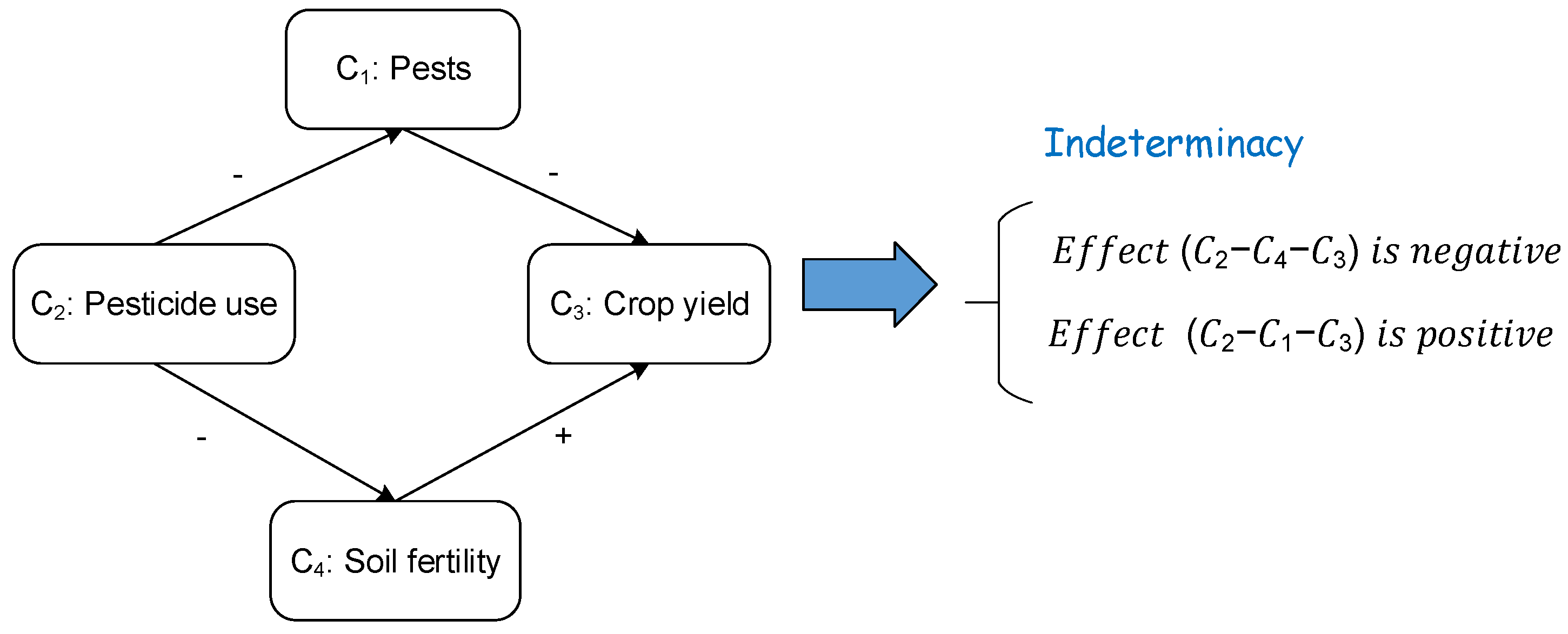
In Axelrod’s approach, the total causal effect on a given concept is elaborated using the sum of all indirect effects cumulated through the different causal paths [42]. For a given indirect path, effect is positive if the path has an even number of negative links, negative otherwise. The total effect is positive if all indirect causal paths lead to positive effects, and the total effect is negative if all indirect causal paths lead to negative effects. However, when some of the indirect causal paths yield negative effects, and others result in positive effects, indeterminacy prevails [43]. The example of Figure 1 shows that the total effect of “Pesticide use” on “Crop yield” is indeterminate.
FCMs, introduced by Kosko in 1986, provide a resolution for indeterminacy in CMs. FCMs introduced fuzziness to Cognitive Maps, by using numeric descriptions (fuzzy binaries) of causal influences instead of positive or negative symbols, “their fuzziness allows hazy degrees of causality between hazy causal objects (concepts)” [18]. Each edge between two concepts Ci and Cj is associated with a weight wij which varies in [−1, 1]. There are three different types of possible causalities between every pair of concepts Ci and Cj:
- ○
- wij > 0, expresses positive causality, that is Ci causally increases Cj.
- ○
- wij < 0, expresses negative causality, that is Ci causally decreases Cj.
- ○
- wij = 0, designates no causality.
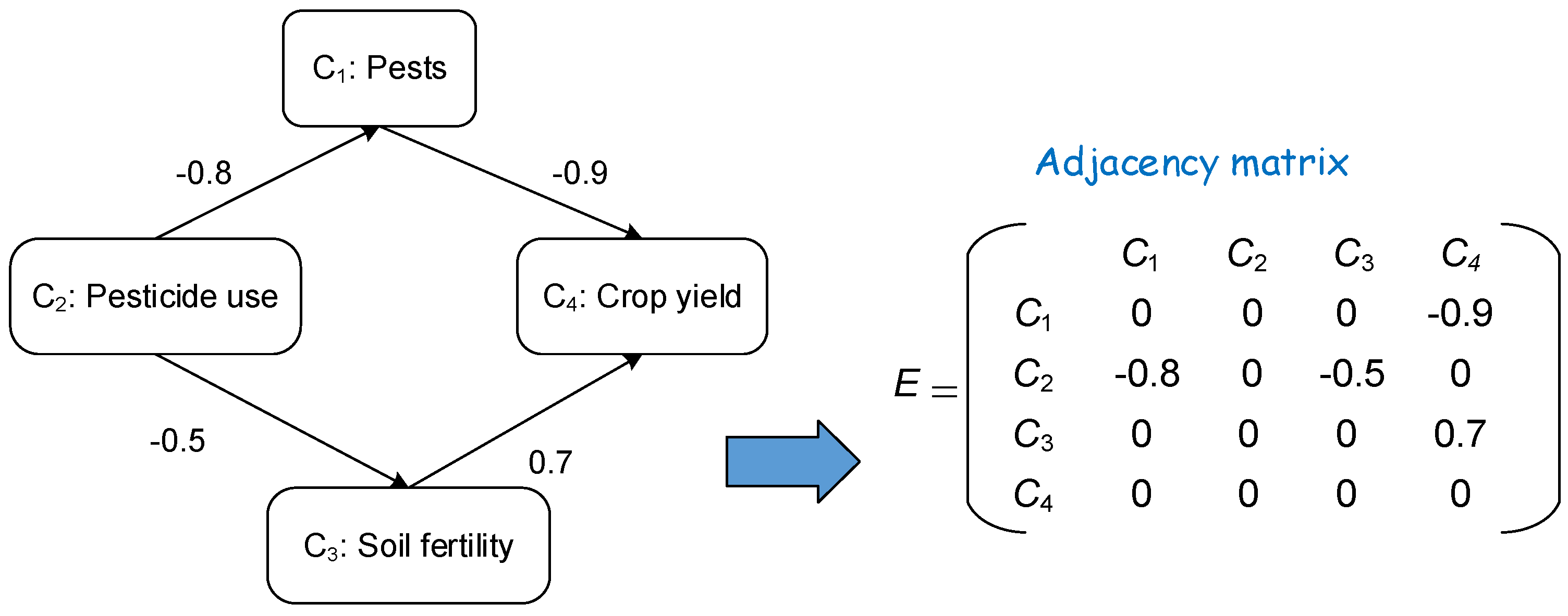
These causal links (also called FCM connections) and their respective weights can be encoded into an NxN (N being the number of concepts) matrix, which is referred to as the Connection or Weight Matrix E. FCM’s graph structure facilitates causal reasoning to study system dynamics, it is a decision support system, where calculations can be made to perform an assessment of the consequences of a specific system state. Since the causal edges are weighted with positive or negative real numbers (wij), then the indirect effect of Ci on Cj on path (i, k1,…,kn, j) is the product wik1 x wk1k2 x …wknj, and the total effect is the sum of the path products. This weighting scheme removes indeterminacy from causal propagation and combination in FCMs [18]. Figure 2 shows an example of a Fuzzy Cognitive Map along with its weight matrix.
FCM forward inference ”allows causal inferences to be made as feedback associative memory recollections”; Kosko calculates each subsequent value of the causal state using previous state and weight matrix multiplication [44]. The concepts take values, which are also called activation levels, between 0 and 1. The State Vector of activations (V) evolves in time according to the influences between concepts. By feeding the FCM model with an initial stimulus V(t) (state vector at time (t)), it can model the evolution of a scenario over time by evolving forward and letting concepts interact with one another. The next state of the system V(t+1) at time (t + 1) is produced by multiplying V(t) by the graph’s weight matrix E. In some FCM implementations, concepts are considered to have memory with a self-feedback link weight of 1. Thus, the next state value of each concept Ci is elaborated, during simulation, by retrieving its value at the previous iteration, and adding it to the propagated weighted values of all factors Cj that have a direct influence on the concept according to Equation (1).
where Ci(k+1) is the activation value of concept Ci at iteration k+1, Ci(k) is the value of node Ci at iteration k, wji is the weight of the cause–effect link between Cj and Ci, and F is a threshold function such as sigmoid, used for squashing the results of the sum between 0 and +1, or between −1 and +1 [45], as shown by Equation (2).
In order to generate projections based on a given simulated scenario, a series of vector-matrix multiplications is performed, until one of the following attractors is reached [18,46]: (i) a fixed point attractor, which means the vector-matrix multiplication converges to an equilibrium state, where the same vector is repeated over a number of iterations, in this case convergence implies that a hidden pattern is discovered; (ii) a limit cycle, which means we obtain few states that get repeated over a number of iterations; or (iii) a chaotic attractor, which means the vector-matrix multiplication does not converge and yields different vectors in each iteration.
Modeling with FCMs offers a number of advantages: (i) they can be used in a participatory approach to model mental views and preferences; (ii) maps produced by different groups of experts can be aggregated to produce a larger and more reliable representative knowledge base, which can help solving knowledge inconsistencies and fostering team-shared objectives, especially in participatory systems involving inter- and multi-disciplinary participants [47,48]; (iii) unlike feed-forward structures such as Rule-based Systems [49], causal reasoning in fuzzy cognitive maps can handle feedback loops; (iv) FCMs inherently support vagueness and ambiguities, and can hence model expert heuristic knowledge; and (v) both quantitative and qualitative data can be integrated into FCM models. FCMs are particularly useful in applications where there is a need to link quantitative modeling with qualitative scenarios, or in which a social learning process needs to be established between stakeholders [21,22,23,50]. They can assist in building models for problems where uncertainty is high, and where data scarcity prevails,
There is a spectrum of FCM implementations in the literature, but most of them focus on depicting causalities between system variables, rather than cause and effect relationships, and FCM inference allows drawing conclusions about what is caused and what is not caused, which is a major limitation in dynamic systems where reasoning is characterized by magnitudes of change and effects [39,51]. Another shortcoming of FCMs is that the links’ weights are forced to a static value in the range [−1, 1], whereas in dynamic systems, the weight would rather be a function of other factors’ influences. Moreover, variables in real models map to a universe of discourse within their minimum and maximum state limits, however, in FCM models, a threshold function normalizes all values between 0 and 1. Furthermore, unlike models built using System Dynamics (SD) [52], FCMs are not dynamic models and cannot model nonlinear relationships, and time-dependent components cannot be formally implemented into FCM models.
2.2. FCM Approach Using Linguistic Fuzzy Influence
Papageorgiou et al. [28] proposed a variant of FCMs, which consists in describing the links’ weights using fuzzy linguistic terms, extracted from fuzzy rules that are collected from domain experts. The approach consists in pooling a number of fuzzy rules from experts for each link of the FCM model to obtain linguistic weights for each interconnection, by considering the consequent of the rule only, ignoring hence the antecedent part.
In order to build the FCM weight matrix, the weights, obtained from all experts, are combined using Fuzzy Logic operators [41]. For every link connecting two concepts, the consequents’ linguistic weights are aggregated by typically using the fuzzy Union operator [31]. The membership function of the Union of two Fuzzy Sets A and B, defined over the set X, with membership functions μA and μB, respectively, is defined by a T-conorm mapping. One of the commonly used mappings is the maximum operator as shown by Equation (3):
Then, a defuzzification method is used to calculate an aggregated numerical weight value of the link. Several methods have been used in practice for defuzzification, the most popular method is the centroid method [31], which calculates the center of gravity of the aggregated fuzzy set as shown by Equation (4):
CoG = ∫μA (x) dx ÷ ∫μA (x) dx
Thus, a numerical weight (wij) is calculated for the link between every pair of concepts Ci and Cj, prior to starting simulations. The simulation is then carried in a normal way, using the forward inference algorithm like in a conventional FCM model. To demonstrate how the linguistic terms are aggregated, let us consider the relation between K (Potassium) and Y (cotton yield), using expert knowledge from [28]:
- 1st Expert:“IF value of concept K is med THEN value of concept Y is medInfer: The influence from concept K towards concept Y is med”
- 2nd Expert:“IF value of concept K is med THEN value of concept Y is highInfer: The influence from concept K towards concept Y is high”
- 3rd Expert:“IF value of concept K is high THEN value of concept Y is very highInfer: The influence from concept K towards concept Y is very high”
The linguistic terms of the consequents (“med”, “high” and “very high”) are summed and an overall linguistic weight is produced, hence transforming the influence into the numerical weight constant WK-Y = 0.65. The process of aggregation and defuzzification is shown by Figure 3.
In the work of Papageorgiou et al. [28], FCMs were also enriched with the unsupervised Nonlinear Hebbian Learning (NHL) algorithm. The technique was used to overcome inadequate knowledge of experts or non-acceptable FCM simulation results. The weight adaptation procedure is based on the Hebbian Learning rule proposed by Oja et al. [53], which has been adapted for FCM models as proposed by Papageorgiou and Groumpos [54].
The main advantage of this approach, over conventional FCMs, is that it allows mapping of expert knowledge by means of fuzzy rules, and it establishes a natural language interface with participants. However, parts of the gathered rules are omitted. The antecedent of a rule would just be ignored, and the only thing that is used to draw a conclusion about the influence is the consequence: is the influence “high”, “medium” or “low”? Only those are used to generate weights. This approach results in building a complex dynamic model with nonlinear relationships, without taking full advantage of expert knowledge in simulating the real world system. Furthermore, although the fuzzy sets have been defined for the yield concept (Y), they are not used in the FCM model, since it produces only normalized values. Hence, it was essential for the experts, in that case study, to determine another threshold value to discriminate between the different yield categories. The experts suggested that 0.85 can be used to distinguish between “low” and “high” yield [28]. If the estimated yield value is less than 0.85, which means that the yield production is less than the 85% of desired cotton production, then yield is categorized as “low”. If the estimated yield value is higher than 0.85, then yield is considered as “high”. Thus, despite the fact that this FCM variant requires a great amount of cognition from experts to produce the fuzzy rules and the membership functions, parts of this knowledge gets ignored, and the inference process is carried in the same way as in a traditional FCM.
2.3. Dynamic Rule-Based Fuzzy Cognitive Maps (DRBFCMs)
FCMs have been heavily used in the literature beyond the simple propagation of causalities as SD models, where the links represent magnitude of change induced by one concept on another one [51]. However, despite the fact that the graph represents a SD system, the developed models used causality-related features of conventional FCMs. First, most FCM implementations make use of fuzzy binaries to quantify the influence exerted by one concept on another by forcing the link’s weight into a static value in the range [−1, 1]. In a SD model, the flows (edges) are the rates at which the stock (state variable) levels are altered; they are expressed in general using differential equations, as functions of other factors’ influences. Second, FCM inference is performed using the mathematical method of Equation (1), where a threshold function such as sigmoid is used to normalize the values within the range [0, 1] because causal reasoning is based on fuzzy binaries. However, variables in a SD model map to a universe of discourse within their minimum and maximum state limits.
DRBFCM was proposed as an alternative to SD using FCMs and FISs [40]. Concepts represent causes or effects that collectively characterize a system state at a given time. Each concept analyzed by experts in the model is divided into a number of intervals, to determine linguistically descriptions corresponding to threshold intervals or possible states it can exist in using membership functions. A general Fuzzy variable called “Variation” is used consistently to represent the influence between concepts. The variation variable has the fuzzy sets such as positively or negatively “low”, “medium”, “high” or “very high”.
The concepts’ set of linguistic terms is used to describe the causal relationships and links between input concepts and outputs using fuzzy “if-then” rules. Every interconnection between two concepts Ci and Cj is represented in the form of a FIS [31]. Each FIS is described using the Fuzzy Control Language (FCL) [55]. In FCL, a FIS is usually composed of one or more Function Blocks (FB). In DRBFCM models, each FB has one input fuzzy variable with membership functions to describe the threshold values of the cause concept, and an output fuzzy variable with membership functions to describe the threshold values of the effect concept, along with the defuzzification method. The FB is also made of one Rule Block (RB), composed of a set of rules, as well as the aggregation, activation and accumulation methods [31]. In DRBFCM, the rules have a single antecedent related to a concept’s state or variation, and a single consequent which is always a variation, representing a perturbation in the output concept. Since FCL supports only rules that map input concept states to output concepts states, the authors modified the FCL grammar to cope with rules describing concept variations [40]. The new FCL grammar has: (i) the “IN^ID” clause added to the subcondition, which is used to specify the causal variation, where “IN” is a keyword and “ID” denotes the cause variable; and (ii) the “ON^ID” clause added to the subconclusion to specify the effect variation, where “ON” is a keyword and “ID” denotes the effect variable:
- Type 1: IF Ci is A THEN Variation is Vi ON Cj
- Type 2: IF Variation is Vi IN Ci THEN Variation is Vj ON Cj
Inference is carried according to an algorithm for combining effects on a given concept, and dealing with feedback. In a given scenario, the state value of a concept is updated by retrieving all incoming connections on that concept, and then the variation induced by every incoming connection is evaluated using fuzzy inference [31,56]. Once the different variations are obtained, the concept’s level is updated by using the state vector and weight matrix multiplication. Concepts are considered to have memory with a self-feedback link weight equal to 1, so the activation value of the concept is updated by recalling its old value and adding it to the summation of weighted input activations. Since DRBFCM models operate on real deterministic values, the influencing concept’s activation value is scaled to the universe of discourse of the output concept using Taylor-Young linear transformation [40].
Compared to the other FCM approaches, DRBFCM models allow reasoning in terms of deterministic concept magnitudes, and DRBFCM inference computes the system variables’ states using quantified perturbations produced by FISs. DRBFCM models are also very authentic to the real models, since the aggregated knowledge is fed into standard FISs, and the consequences of the rules are also used to produce a link’s weight, but provided that the antecedent is fulfilled: which concept affects the yield, and to which extent?
An empirical comparison between FCM and DRBFCM models, in application of cotton yield prediction in PA, can be found in [57]. DRBFCM was evaluated for 360 cases, measured for three years (2001, 2003 and 2006), in a 5 ha experimental cotton field. The results revealed an accuracy of predictions of 85.55%, 87.22% and 73.33%, against 73.80%, 67.20% and 69.65% for the conventional FCM model, and against 75.55%, 68.86% and 71.32% for the FCM model with the Nonlinear Hebbian Learning algorithm, for the years 2001, 2003 and 2006, respectively. DRBFCM proved, in this case study, to predict more accurately the yield while being faithful to the real world model.
In DRBFCM, Fuzzy Logic caters for uncertainties and facilitates representation of non-monotonic cause–effect relationships, by mapping dynamically causal node states to effect node states in FCM models. This method allows representation of non-monotonic relationships, without the need for capturing the functional connections between concepts of the real system by means of complex mathematical equations. However, producing a robust DRBFCM model, with enough cognition to interrogate the different facades of a system, will result in increasing its complexity. The more concepts added to the model, the higher the number of “if-then” rules to be elicited from experts to model the system’s complexities, and to be evaluated by the model.
2.4. Simulation with SimulDRBFCM Models
In this work, we propose SimulDRBFCM models as an approach that allows managers to generate raw scenarios and create simulations. Similar to DRBFCMs, the links’ weights are determined dynamically using FISs at simulation time. However, since the focus is on building simulations starting from a baseline scenario to study the effect of decreasing fertilizers on the yield production, we make the assumption that the state vector depicts degrees of concept change not deterministic concept values. The link’s weight designates the strength of the effect induced by a change in a cause concept (system driver) on an effect concept, and not fuzzy binaries about uncertain causal relationships. Hence, a SimulDRBFCM model is a DRBFCM model where reasoning is performed in terms of magnitudes of changes. In order to construct a SimulDRBFCM model, experts are requested to identify the main factors that describe the system, and the weight of causal influence between the concepts using fuzzy rules.
If the maps are designed using multiple experts, the rules collected from the different participants are simply compiled into a single rule block. As a result of combining knowledge from different participants, the aggregated rule block might contain conflicting rules. These are aggregated as part of the inference algorithm, which reflects variation in supported human perceptions.
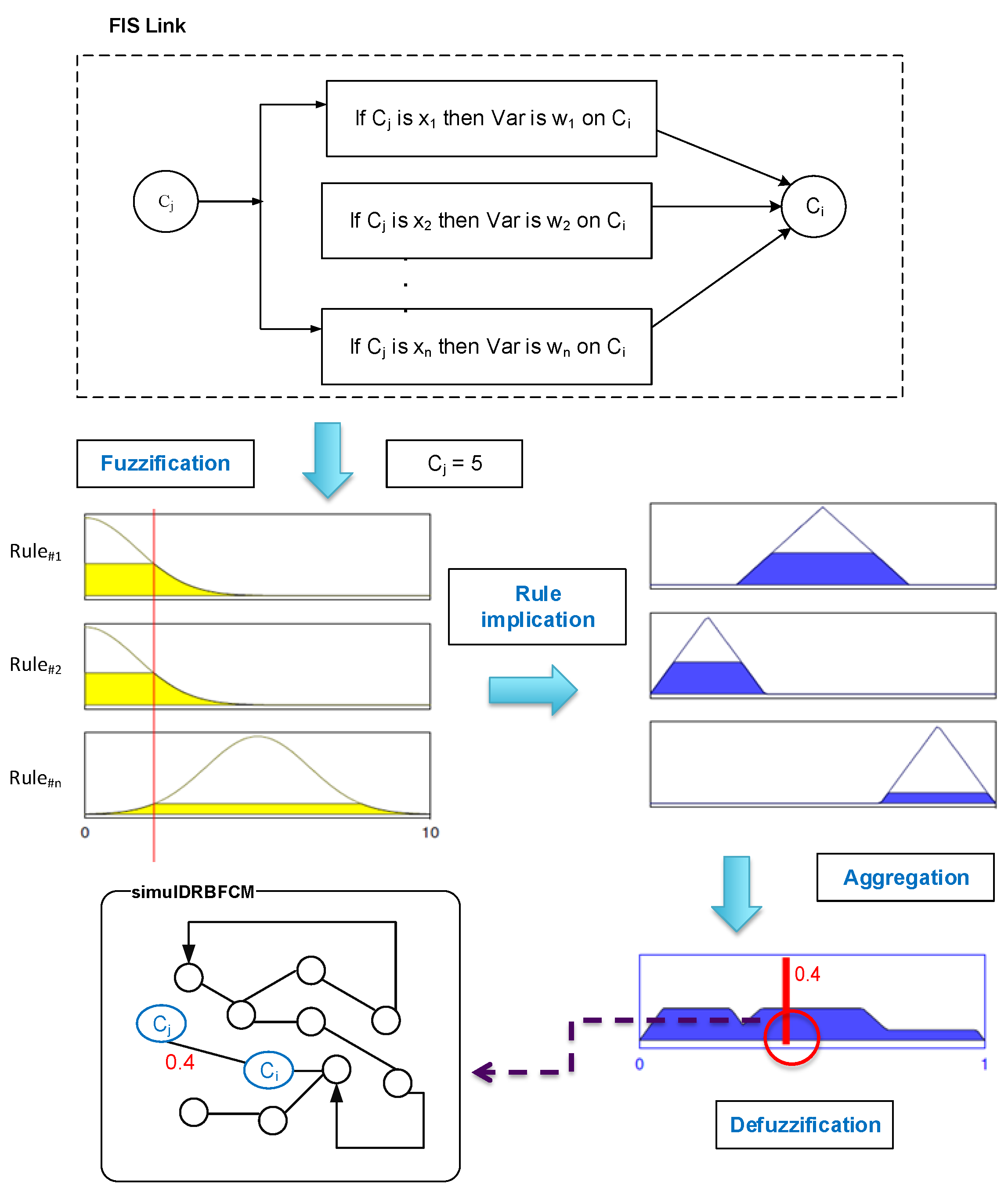
Like in DRBFCMs, the link’s weight is updated dynamically, during every iteration of a given simulation, using fuzzy inference. Since every connection between two concepts is a FIS, we make use of the Mamdani’s inference type to compute the influence weight [56]. We opted for Mamdani’s approach because it is more intuitive and well suited to human input. This approach is known for its simple structure and inference; the implication method used is the “min” and the rule composition method is “max–min” [31]. Using the fuzzy inference process, the FCM is stimulated with concepts’ levels, hence we need only rules of Type 1. Crisp input is fuzzified using membership functions of the cause variable to produce a membership grade in qualifying linguistic sets. The application of the rule implication method maps the rule strength from the antecedent into the consequent. The outputs of the rules are then aggregated using a fuzzy union operator. The resulting aggregated fuzzy set is then defuzzified using the centroid method. Hence, an overall crisp numerical weight is produced to show the aggregate influence for one cause–effect link. The process of generating a link’s weight is illustrated in Figure 4.
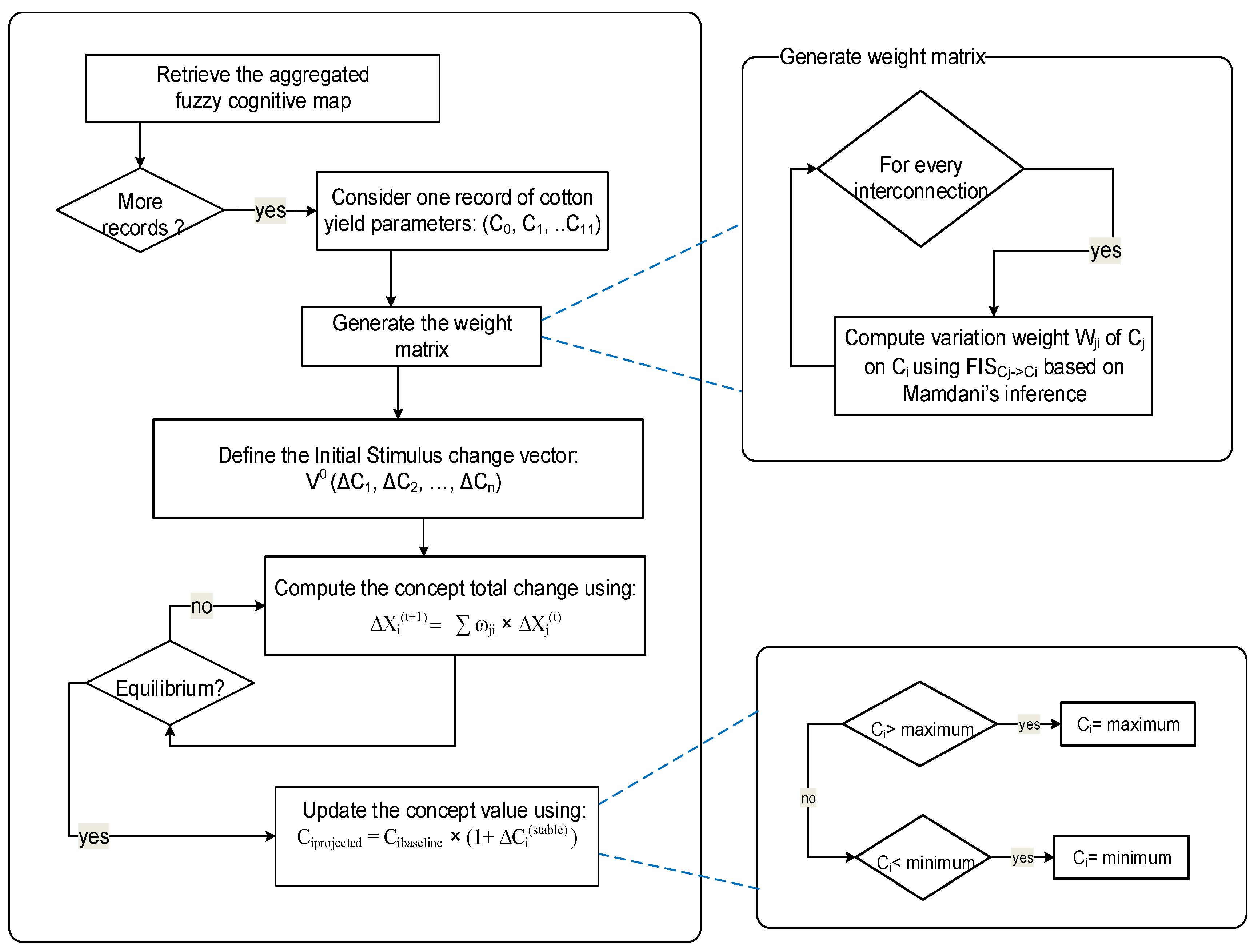
To describe how the system may react to changes in system drivers, experts are requested to identify the main system drivers and essentially those that are uncertain. In a given scenario, to explore the direct effect of the change in the value of a driver variable, let us say Cj of magnitude ΔCj, on the value of an output variable Ci, with a potential change of magnitude ΔCi, we stimulate the system with magnitudes of change. Inference is carried according to an algorithm for combining effects on a given concept, and dealing with feedback using FCM inference. SimulDRBFCM inference computes the new system variables’ states using quantified perturbations produced by FCMs that are weighted using FISs. The inference algorithm is summarized in Figure 5.
The vector of changes takes values between −1 and 1, where zero means no change assumed for the corresponding concept, and ±1 means that the concept is stimulated with ±100% increase or decrease. The vector evolves in time according to the influences between concepts, the change vector X(t+1) is produced by multiplying the previous change (X(t)) by the graph’s weight adjacency matrix (E).
The next concept change ΔCi is calculated during simulation, by computing the propagated weighted estimated change of all concepts Cj that have a direct influence on the concept Ci, according to Equation (5).
The assumption is that we are studying the changes a system might experience starting from a baseline scenario, so the initial concept state is a known value, hence the projected value of any concept can be inferred using Equation (6).
In our approach, we assume a linear transfer function to map the changes from the causal nodes to the effect node. When more expertise is available, nonlinear SD transformations can be used [52].
It should be also noted that concepts map to a universe of discourse between their minimum and maximum state limits using fuzzy variables. We operate hence on real values, concept states are not arbitrarily altered using squashing functions, but are rather compared against their universe of discourse.
The approach is particularly useful when the aim is to explore the change produced by certain drivers rather than predicting the absolute magnitude of a quantity. In PA, one might rather be interested into gaining insights about effects of increasing or decreasing fertilizer nutrients on crop yield.
Compared to DRBFCM, the methodological enhancement brought by SimulDRBFCM models reduces the number of rules needed to model the system’s dynamics, since only rules of Type 1 mapping concepts’ input states to the output’s perturbation are used to produce simulations; the normal FCM forward inference is used to compute intermediate perturbations and derive the steady state of concept changes.
3. Case Study: Cotton Yield SimulDRBFCM Model
3.1. Cotton Yield Knowledge
The knowledge and data were obtained from the work of Papageorgiou et al. [28] to predict cotton yield. Three experts contributed to the design of the cotton yield model. One of the experts is a soil scientist from Technological Educational Institute of Larissa, Greece, the second one is also a soil scientist from the Laboratory of Regional Soil Analysis and Agricultural Applications of Larissa, Greece, and the third one is a cotton farmer.
The experts stated that there are eleven soil parameters that can be used to determine cotton yield as shown in Table 1. The experts described the soil parameters and their threshold values using membership functions as depicted in Table 2. The list of fuzzy rules aggregated from the three experts is shown in Table 3, where “VAR” is the variation fuzzy variable.
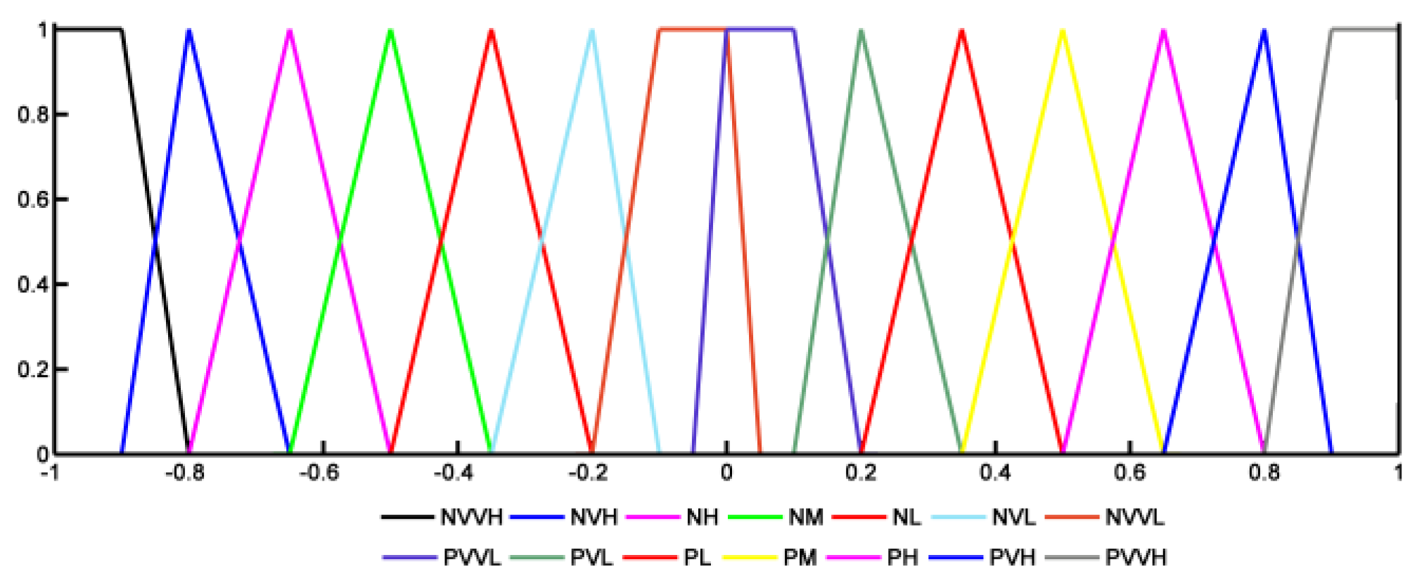
The degree of variation induced by one concept on another one is elaborated through the fuzzy variable “Influence” of Figure 6, with the following fuzzy sets (“VVH: very very high”, “VH: very high”, “H: high”, “M: medium”, “L: low”, “VL: very low”, “VVL: very very low”). The influence can be positive or negative.
3.2. Cotton Yield Data
The used data consists of 360 entries measured for the years 2001, 2003 and 2006, as collected in a 5 ha field at Myrina, Karditsa prefecture, Central Greece. As explained in the work of Papageorgiou et al. [28], cotton yield mapping was performed using a FarmscanTM yield monitor installed on a two row John DeereTM cotton picker [58]. After field harvesting was completed, a calibration procedure was performed to improve the yield estimation [59]. The FCM model has been developed based on a raster data GIS approach, i.e., the data was stored in a two-dimensional matrix that represents the spatial distribution of every factor in the field. Each cell of the matrix corresponds to an area of 10 × 10 m, which is the spatial resolution of the yield data model.
3.3. Cotton Yield Simulations
We developed the cotton yield model following the SimulDRBFCM modeling approach described in the previous section. A recapitulation of weights for the traditional FCM and SimulDRBFCM models are shown in Table 4, where we can clearly see that the influence of K is lower in SimulDRBFCM (WK-Y = 0.22 ± 1.88 × 10⁻⁴), compared to the traditional FCM (WK-Y = 0.6). The low influence produced by the SimulDRBFCM model seems to make sense as K produces a “high” variation when it is classified as “high” or “very high”. Nevertheless, by looking at the 360 cases of cotton yield data, K was classified as either “medium” or “low” all the time. Hence, SimulDRBFCM cotton yield model seems to generate weights that are coherent with the model structure and collected knowledge, and it produces weights that can be interpreted by tracing the rules that contributed to the results.
In order to reduce the uncertainties about how variable fertilizer rate technology might affect cotton yield, we generated a number of raw scenarios to study the effect of decreasing K, P and N at fixed intervals. The results were combined with the 360 cases of cotton yield data to generate 1331 different scenarios. After convergence of the SimulDRBFCM model, the outcome of the different scenarios were compared with the baseline scenario, which is made of the original cotton yield data, to understand how cotton yield relatively changes under the condition of decreasing K, P and N. The generated yield was compared with the considered normal yield in Greece, which is approximately 2.5 t ha−1 under normal weather conditions. Table 5 shows some of the results under four scenarios, where the target acceptable decrease in cotton yield production was set to a maximum of 2.5%, 5%, 7.5%, and 10%. In a policy development exercise, the target could be set, for example, by a cost–benefit analysis or by stakeholders.
There are different responses to the cotton yield category in relation to initial soil K, P and N changes. From the results, it can be seen that decreasing K and P by at most 10% and keeping N at the same level does not decrease the yield by more than 2.5%. When the target maximum yield decrease is 5%, we can see that among the three factors, P and N seem to play a more crucial role in making the yield drop quite significantly. If N or P is decreased nearly by half, the yield decreases by at most 4.8%. Otherwise, decreasing the three factors between 10% and 20% also does not decrease the yield by more than 5.06%, while the yield category decreases from “high” to “low” in 10 cases of the 360 cotton yield data (i.e., nearly 2.77%).
If the target is to achieve no more than 7.5% yield decrease, N can be decreased by 70% while keeping the other factors at the same level, or by cutting P by 40%, or by cutting N by 30% and decreasing one of the other factors between 10% and 20%, or by cutting N by 30% and decreasing one of the other factors between 10% and 20%. It can be achieved also by cutting K by 40% and one of the other factors by 10%. In this case, the yield category decreases from “high” to “low” in 21 cases of the 360 cotton yield data (i.e., nearly 5.83%).
Another significant result is that the decrease in yield plateaus when the total decrease in nutrients reaches a total of 70%. We can notice that even by decreasing K by 60%, P by 80% and N by 90%, the yield decreases by no more than 10%. In this case, the yield category decreases from “high” to “low” in 28 cases (i.e., nearly 7.77%). This suggests that under conditions of limited nutrient applications, the crop makes maximum use of the nutrient that is taken up.
With respect to the original 360 cases of cotton yield data, used as a baseline scenario, it should be noted that it is characterized by “low” to “medium” P, K, and N. The three factors were never classified as “high” or “very high”. According to the knowledge collected from experts, too much nutrients can be harmful to the yield, e.g., N is needed in fair amounts, and too much N can lower the production. Thus, in cases where simulations are run using a baseline scenario where K, P, or N factors are classified as “high” in the original data set, dropping these factors during a simulation to a lower category such as “medium” might even increase the yield and hence the profitability.
The general fertilizer response characteristics based on simulations are summarized in Table 6.
Under the first scenario (2.5% decrease), the mean Nitrogen content is 11.02 ± 3.36, the mean Potassium content is 0.27 ± 6.34 × 10⁻², and the mean Phosphorus content is 15.83 ± 1.97. These values appear to be characteristic, independently from growing conditions, of a yield mean of 248.16 ± 9.91× 10⁻¹, which corresponds nearly to the normal yield value in Greece.
Similarly, under the second scenario (5% decrease), the mean Nitrogen content is 9.94 ± 3.06, the mean Potassium content is 0.29 ± 8.61 × 10⁻², and the mean Phosphorus content is 15.85 ± 2.62. These values appear to be characteristic of a yield mean of 245.59 ± 2.51.
Under the third scenario (7.5% decrease), the mean Nitrogen content is 9.43 ± 3.52, the mean Potassium content is 0.29 ± 8.45 × 10⁻², and the mean Phosphorus content is 16.71 ± 5.65. These values appear to be characteristic of a yield mean of 243.51 ± 4.38.
Under the fourth scenario (10% decrease), the mean Nitrogen content is 9.08 ± 4.11, the mean Potassium content is 0.29 ± 9.01 × 10⁻², and the mean Phosphorus content is 16.01 ± 5.87. These values appear to be characteristic of a yield mean of 240.80 ± 5.97.
The results are, of course, to be combined with further knowledge about crop variables. The current cotton yield model characterizes mainly the influence induced by soil parameters on yield, and it is lacking strong feedback links and dynamics between the different nutrients themselves. For example, insufficient K may lead to reduced N uptake, hence scenarios that decrease K should be handled carefully. With respect to fertilization, another issue lies in plant-specific application of N taking into account the soil moisture available to the plant. The current expert system does not contain knowledge that describes the influence of moisture on crop production.
3.4. Statistical Significance Tests
To ensure the scientific validity of the SimulDRBFCM method, all analyzed scenario outcomes have been clustered into groups, performing according to the 2.5%, 5%, 7.5% and 10% yield decreases. Thus, the aforementioned groups form four spreadsheets that include the id-cases and all dependent, independent and not participating in the study variables. However, the spreadsheet that covers all yield decreases up to 10% includes all smaller decrease cases therefore acting as a superset of all cases. This corresponds to 2847 distinct combinations of either K or P, or N decrease and the computed outcomes of yield decrease and the percentage of this decrease criterion. Based on the last set of cases, we performed several statistical tests, by concentrating on the statistical significance of our simulation outcomes [60]. The purpose of this experimental testing is to assess the true prediction quality of the SimulDRBFCM model for the simulations above. The statistical significance is an estimate of the degree, to which the SimulDRBFCM predictions’ quality lies within a confidence interval around the measurement on the test sets. A commonly used level of reliability of the result is 95%, also written as p = 0.05, called p-level. Given the set of n = 2847 distinct cases of interest, we can compute the sample mean and variance of the individual simulation scores (i.e., |actual_yield − computed_yield|), but what we really are interested in however is the true mean (μ) of the simulation set. Let us assume that the SimulDRBFCM model scores for the yield decrease are distributed according to the normal distribution. This implies that any simulation score is independent from other simulation scores. Since we do not know the true mean μ and variance σ2, we cannot model the distribution of simulation scores with the normal distribution. However, we can use Student’s t-distribution [61], which approximates the normal distribution for a large simulation set n.
Relative to the confidence interval [μ − d, μ + d] around the mean yield decrease simulation score, the SimulDRBFCM model quality lies within the confidence interval with a probability q. The relationship between the degree of statistical significance and the confidence interval is shown in Figure 7, which really expresses the statistical significance by the fraction of the area under the curve that is shaded.
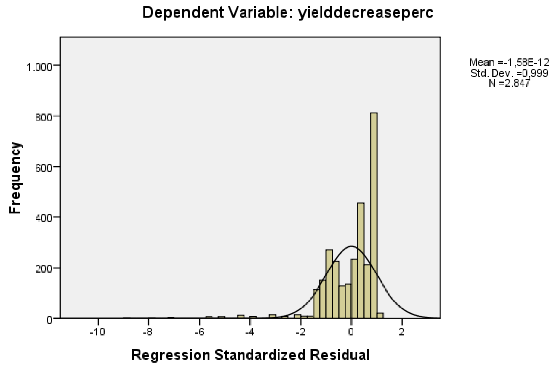
The confidence interval is indicated by the boundaries on the x-axis. The functional mapping between a confidence interval [] and the probability q can be obtained by integrating over the distribution [62]. However, in case of Student’s t-distribution, the solution to this does not exist in closed form, but we can use numerical methods. According to the above mentioned explanation, we performed in SPSS Statistics for Windows, version 16.0 (SPSS Inc., Chicago, USA) an examination of the distribution used which is found to be near Student’s t-distribution as shown in Figure 8.
This allowed us to perform three non-parametric pairwise sample tests spanning from 95% to 99% confidence intervals that justify the true statistical significance of our model. These tests show that there is no significant difference when going over the confidence interval of 95% which is the most popular and used one. Note that the mean, the standard deviation, the standard error mean, and the upper and lower bounds remain the same for all cases since they refer to the same sample and only the t-values change (see Table 7, Table 8 and Table 9).
To cover the relevant abnormality in the distribution shown in Figure 8 we also performed a Mann–Whitney U-test on all the cases and all the scenarios under the full extension of our simulation study. The Mann–Whitney U is a non-parametric test used to assess for significant differences in a scale or ordinal dependent variable by a single dichotomous independent variable. It is the non-parametric equivalent of the independent samples t-test [63]. More specifically, we chose to investigate the p-value in the statistical significance for the variables of K-reduction, P-reduction, N-reduction and yield-reduction predicted by the model. For this reason, we have used the dichotomous independent variable to be the transition from the state of high-yield to low-yield according to the description in the previous subsection.
For this test, we used all 1331 scenarios each one containing the 360 cases of yield predictions. The Mann–Whitney U-test was also performed in SPSS and its results are shown by Table 10 and Table 11. The most important finding is that the (two-tailed) Asymptotic Sig. is 0.00 for yield-reduction, K-reduction and P-reduction, giving a value smaller than the original p-value.
This result confirms that the yield reduction, K reduction and P reduction measures are highly significant (p < 0.001). However, for these data, the Mann–Whitney test is not significant (two-tailed) for the N Reduction scores performed in yield prediction.
4. Conclusions and Future Work
In this work, we proposed the SimulDRBFCM modeling method, which is a Fuzzy Cognitive Map where relationships between concepts are expressed in the form of Fuzzy Inference Systems that dynamically determine the influence between concepts, while running a simulation for a specific scenario. The model is hence capable of simulating change in system output when stimulated with change in the main system drivers. Modeling with SimulDRBFCM offers also a number of advantages besides simulating change. In comparison to a traditional FCM model, SimulDRBFCM is more faithful to the real world model, since the knowledge collected from the experts is fed into a standard inference system to map adequately and dynamically an input space into an output space during simulation. Furthermore, SimulDRBFCM generates predictions that can be interpreted by tracing the rules that contributed to the results.
The knowledge-based approach can be very helpful to managers and stakeholders in PA because it increases system understanding, and reduces the uncertainties about the way a given model may react to changes in system drivers. This is interesting because it helps avoiding pitfalls caused by ignorance, and teaches skills that are likely to last beyond the modeling process.
The adoption of PA technologies should be supported by the development of appropriate regulations and policies, and the establishment of coordination bodies and linkages with national strategies. In this perspective, SimulDRBFCM has the potential to bring science to the process of strategic planning in PA by offering tools to link management storylines to quantitative scenarios. It allows building simulations with transparent and traceable results that are consistent and reproducible. This is interesting, from policymakers’ perspective, because the evaluation of the impact of different PA management options, from an integrated perspective, before their establishment can offer cues and may reduce costs, efforts as well as the risk of failure.
Moreover, the proposed approach offers an opportunity to optimize crop quality and yield production. Yield and quality are influenced by soil fertility which can vary from one field grid to another one. The method would allow farmers to identify those parcels of potential low production, and take actions proactively by applying the needed amounts of fertilizers to achieve optimal production.
The illustrative case study was built using knowledge collected from multiple experts. The proposed approach was successfully applied to generate the aggregate system complexities, facilitating thus conciliation of opinions and conflict resolution. It is also interesting because it ensures that interventions will have more credibility, which can help increase the uptake of precision agriculture management by stakeholders and farmers. We applied the approach, to generate different scenarios to predict how cotton yield related to K, P and N changes. In this study, the results of simulations showed that decreasing the three nutrients by half does not decrease yield by more than 10%, which might suggest that N, K, and P amounts can be reviewed in respect to fertilizer recommendations without compromising the yield production. Applying only the necessary nitrogen rates to achieve an optimal crop yield can help decreasing adverse environmental effects, and hence ensure environmental protection. PA can particularly alleviate nitrate contamination in groundwater, which is a major consideration in the contamination of many of the world’s water streams. Moreover, if a famer has precise information on nutrients needed on each parcel, variable rate application could reduce costs and increase profitability, based on the assumption that the achieved net savings offset the cost of any additional labor or acquisition of technologies. Hence, while reducing the environmental footprint, PA can also help boosting economic efficiency in on-farm activities.
As future work, we would like to combine the results with a cost–benefit analysis to gain insights into the actual profits that can be achieved by using precision agriculture. We would like also to generate more scenarios and simulations using data with higher variability, and taking into consideration crop sensitivity to weather conditions, nutrient interdependencies, losses and recovery.
Author Contributions
A.M. and E.P. conceived and designed the experiments; A.M. performed the experiments; A.M. and KK. analyzed the data; A.M, E.P, K.K and T.R. wrote the paper.
Conflicts of Interest
The authors declare no conflict of interest.
References
- Biermacher, J.T.; Brorsen, B.W.; Epplin, F.M.; Solie, J.B.; Raun, W.R. The economic potential of precision nitrogen application with wheat based on plant sensing. Agric. Econ. 2009, 40, 397–407. [Google Scholar] [CrossRef]
- Aubert, B.A.; Schroeder, A.; Grimaudo, J. IT as enabler of sustainable farming: An empirical analysis of farmers’ adoption decision of precision agriculture technology. Decis. Support Syst. 2012, 54, 510–520. [Google Scholar] [CrossRef]
- Lencsés, E.; Takács, I.; Takács-György, K. Farmers’ Perception of Precision Farming Technology among Hungarian Farmers. Sustainability 2014, 6, 8452–8465. [Google Scholar] [CrossRef]
- Seelan, S.K.; Laguette, S.; Casady, G.M.; Seielstad, G.A. Remote sensing applications for precision agriculture: A learning community approach. Remote Sens. Environ. 2003, 88, 157–169. [Google Scholar] [CrossRef]
- Bongiovanni, R.; Lowenberg-Deboer, J. Precision Agriculture and Sustainability. Precis. Agric. 2004, 5, 359–387. [Google Scholar] [CrossRef]
- Lowenberg-DeBoer, J.; Swinton, S. Economics of site-specific management in agronomic crops. In The State of site-Specific Management for Agriculture (Thestateofsites); American Society of Agronomy, Crop Science Society of America, and Soil Science Society of America (ASA, CSSA, and SSSA): Madison, WI, USA, 1997; pp. 369–396. [Google Scholar]
- Batte, M.T. Factors influencing the profitability of precision farming systems. J. Soil Water Conserv. 2000, 55, 12–18. [Google Scholar]
- Arnholt, M.; Batte, M.T.; Prochaska, S. Adoption and Use of Precision Farming Technologies: A Survey of Central Ohio Precision Farmers; Report Series: AEDE-RP-0011-01; Department of Agricultural, Environmental and Development Economics, The Ohio State University: Columbus, OH, USA, 2001. [Google Scholar]
- Rider, T.W.; Vogel, J.W.; Dille, J.A.; Dhuyvetter, K.C.; Kastens, T.L. An economic evaluation of site-specific herbicide application. Precis. Agric. 2006, 7, 379–392. [Google Scholar] [CrossRef]
- Tey, Y.S.; Brindal, M. Factors influencing the adoption of precision agricultural technologies: A review for policy implications. Precis. Agric. 2012, 13, 713–730. [Google Scholar] [CrossRef]
- Reichardt, M.; Jürgens, C.; Klöble, U.; Hüter, J.; Moser, K. Dissemination of precision farming in Germany: Acceptance, adoption, obstacles, knowledge transfer and training activities. Precis. Agric. 2009, 10, 525. [Google Scholar] [CrossRef]
- Bramley, R.G.V. Lessons from nearly 20 years of Precision Agriculture research, development, and adoption as a guide to its appropriate application. Crop Pasture Sci. 2009, 60, 197–217. [Google Scholar] [CrossRef]
- Torbett, J.C.; Roberts, R.K.; Larson, J.A.; English, B.C. Perceived importance of precision farming technologies in improving phosphorus and potassium efficiency in cotton production. Precis. Agric. 2007, 8, 127–137. [Google Scholar] [CrossRef]
- Pierpaoli, E.; Carli, G.; Pignatti, E.; Canavari, M. Drivers of Precision Agriculture Technologies Adoption: A Literature Review. Procedia Technol. 2013, 8, 61–69. [Google Scholar] [CrossRef]
- McBride, W.D.; Daberkow, S.G. Information and the adoption of precision farming technologies. J. Agribus. 2003, 21, 21–38. [Google Scholar]
- Puerto, P.; Domingo, R.; Torres, R.; Pérez-Pastor, A.; García-Riquelme, M. Remote management of deficit irrigation in almond trees based on maximum daily trunk shrinkage. Water relations and yield. Agric. Water Manag. 2013, 126, 33–45. [Google Scholar] [CrossRef]
- De la Rosa, J.M.; Conesa, M.R.; Domingo, R.; Aguayo, E.; Falagán, N.; Pérez-Pastor, A. Combined effects of deficit irrigation and crop level on early nectarine trees. Agric. Water Manag. 2016, 170, 120–132. [Google Scholar] [CrossRef]
- Kosko, B. Fuzzy cognitive maps. Int. J. Man-Mach. Stud. 1986, 24, 65–75. [Google Scholar] [CrossRef]
- Gray, S.A.; Gray, S.; De Kok, J.L.; Helfgott, A.E.; O’Dwyer, B.; Jordan, R.; Nyaki, A.; Analyzing, F. Using fuzzy cognitive mapping as a participatory approach to analyze change, preferred states, and perceived resilience of social-ecological systems. Ecol. Soc. 2015, 20, 11. [Google Scholar] [CrossRef]
- Özesmi, U.; Özesmi, S.L. Ecological models based on people’s knowledge: A multi-step fuzzy cognitive mapping approach. Ecol. Model. 2004, 176, 43–64. [Google Scholar] [CrossRef]
- Van Vliet, M.; Kok, K.; Veldkamp, T. Linking stakeholders and modellers in scenario studies: The use of Fuzzy Cognitive Maps as a communication and learning tool. Futures 2010, 42, 1–14. [Google Scholar] [CrossRef]
- Kontogianni, A.D.; Papageorgiou, E.I.; Tourkolias, C. How do you perceive environmental change? Fuzzy Cognitive Mapping informing stakeholder analysis for environmental policy making and non-market valuation. Appl. Soft Comput. 2012, 12, 3725–3735. [Google Scholar] [CrossRef]
- Samarasinghe, S.; Strickert, G. Mixed-method integration and advances in fuzzy cognitive maps for computational policy simulations for natural hazard mitigation. Environ. Model. Softw. 2013, 39, 188–200. [Google Scholar] [CrossRef]
- Kafetzis, A.; McRoberts, N.; Mouratiadou, I. Using Fuzzy Cognitive Maps to Support the Analysis of Stakeholders’ Views of Water Resource Use and Water Quality Policy. In Fuzzy Cognitive Maps: Advances in Theory, Methodologies, Tools and Applications; Glykas, M., Ed.; Springer: Berlin/Heidelberg, Germany, 2010; pp. 383–402. [Google Scholar]
- Giordano, R.; Vurro, M. Fuzzy Cognitive Map to Support Conflict Analysis in Drought Management. In Fuzzy Cognitive Maps: Advances in Theory, Methodologies, Tools and Applications; Glykas, M., Ed.; Springer: Berlin/Heidelberg, Germany, 2010; pp. 403–425. [Google Scholar] [CrossRef]
- Papageorgiou, E.I.; Salmeron, J.L. A Review of Fuzzy Cognitive Maps Research During the Last Decade. IEEE Trans. Fuzzy Syst. 2013, 21, 66–79. [Google Scholar] [CrossRef]
- Jetter, A.J.; Kok, K. Fuzzy Cognitive Maps for futures studies—A methodological assessment of concepts and methods. Futures 2014, 61, 45–57. [Google Scholar] [CrossRef]
- Papageorgiou, E.I.; Markinos, A.; Gemptos, T. Application of fuzzy cognitive maps for cotton yield management in precision farming. Expert Syst. Appl. 2009, 36, 12399–12413. [Google Scholar] [CrossRef]
- Papageorgiou, E.I.; Aggelopoulou, K.D.; Gemtos, T.A.; Nanos, G.D. Yield prediction in apples using Fuzzy Cognitive Map learning approach. Comput. Electron. Agric. 2013, 91, 19–29. [Google Scholar] [CrossRef]
- Jayashree, L.S.; Palakkal, N.; Papageorgiou, E.I.; Papageorgiou, K. Application of fuzzy cognitive maps in precision agriculture: A case study on coconut yield management of southern India’s Malabar region. Neural Comput. Appl. 2015, 26, 1963–1978. [Google Scholar] [CrossRef]
- Ross, T.J. Fuzzy Logic with Engineering Applications; Wiley: New York, NJ, USA, 2009. [Google Scholar]
- Srinivasan, S.P.; Malliga, P. A new approach of adaptive Neuro Fuzzy Inference System (ANFIS) modeling for yield prediction in the supply chain of Jatropha. In Proceedings of the 2010 IEEE 17th International Conference on Industrial Engineering and Engineering Management, Xiamen, China, 29–31 October 2010; pp. 1249–1253. [Google Scholar] [CrossRef]
- Naderloo, L.; Alimardani, R.; Omid, M.; Sarmadian, F.; Javadikia, P.; Torabi, M.Y.; Alimardani, F. Application of ANFIS to predict crop yield based on different energy inputs. Measurement 2012, 45, 1406–1413. [Google Scholar] [CrossRef]
- Khashei-Siuki, A.; Kouchkzadeh, M.; Ghahraman, B. Predicting dryland wheat yield from meteorological data using expert system, Khorasan Province, Iran. J. Agric. Sci. Technol. 2011, 13, 627–640. [Google Scholar]
- Hosseinpourtehrani, M.; Ghahraman, B. Optimal reservoir operation for irrigation of multiple crops using Fuzzy logic. Asian J. Appl. Sci. 2011, 4, 493–513. [Google Scholar]
- Tremblay, N.; Bouroubi, M.Y.; Panneton, B.; Guillaume, S.; Vigneault, P.; Bélec, C. Development and validation of fuzzy logic inference to determine optimum rates of N for corn on the basis of field and crop features. Precis. Agric. 2010, 11, 621–635. [Google Scholar] [CrossRef]
- Mazloumzadeh, S.M.; Shamsi, M.; Nezamabadi-Pour, H. Fuzzy logic to classify date palm trees based on some physical properties related to precision agriculture. Precis. Agric. 2010, 11, 258–273. [Google Scholar] [CrossRef]
- Tagarakis, A.; Koundouras, S.; Papageorgiou, E.I.; Dikopoulou, Z.; Fountas, S.; Gemtos, T.A. A fuzzy inference system to model grape quality in vineyards. Precis. Agric. 2014, 15, 555–578. [Google Scholar] [CrossRef]
- Carvalho, J.P.; Tomé, J.A.B. Fuzzy Mechanisms for Qualitative Causal Relations. In Views on Fuzzy Sets and Systems from Different Perspectives: Philosophy and Logic, Criticisms and Applications; Seising, R., Ed.; Springer: Berlin/Heidelberg, Germany, 2009; pp. 393–415. [Google Scholar] [CrossRef]
- Mourhir, A.; Rachidi, T.; Papageorgiou, E.I.; Karim, M.; Alaoui, F.S. A cognitive map framework to support integrated environmental assessment. Environ. Model. Softw. 2016, 77, 81–94. [Google Scholar] [CrossRef]
- Zadeh, L.A. Fuzzy sets. Inf. Control 1965, 8, 338–353. [Google Scholar] [CrossRef]
- Axelrod, R. Structure of Decision: The Cognitive Maps of Political Elites; Princeton University: Princeton, NJ, USA, 1976. [Google Scholar]
- Calais, G. Fuzzy cognitive maps theory: Implications for interdisciplinary reading: National implications. FOCUS Coll. Univ. Sch. 2008, 2, 1–16. [Google Scholar]
- Kosko, B. Adaptive inference in fuzzy knowledge networks. In Proceedings of the First IEEE International Conference on Neural Networks, San Diego, CA, USA, 21–24 June 1987. [Google Scholar]
- Tsadiras, A.K. Comparing the inference capabilities of binary, trivalent and sigmoid fuzzy cognitive maps. Inf. Sci. 2008, 178, 3880–3894. [Google Scholar] [CrossRef]
- Taber, R. Knowledge processing with Fuzzy Cognitive Maps. Expert Syst. Appl. 1991, 2, 83–87. [Google Scholar] [CrossRef]
- Kosko, B. Fuzzy knowledge combination. Int. J. Intell. Syst. 1986, 1, 293–320. [Google Scholar] [CrossRef]
- Kosko, B. Hidden patterns in combined and adaptive knowledge networks. Int. J. Approx. Reason. 1988, 2, 377–393. [Google Scholar] [CrossRef]
- Adriaenssens, V.; Baets, B.D.; Goethals, P.L.M.; Pauw, N.D. Fuzzy rule-based models for decision support in ecosystem management. Sci. Total Environ. 2004, 319, 1–12. [Google Scholar] [CrossRef]
- Kok, K. The potential of Fuzzy Cognitive Maps for semi-quantitative scenario development, with an example from Brazil. Glob. Environ. Chang. 2009, 19, 122–133. [Google Scholar] [CrossRef]
- Helfgott, A.; Lord, S.; Bean, N.; Wildenberg, M.; Gray, S.; Gray, S.; Vervoort, J.; Kok, K.; Ingram, J. Working Paper 1: Clarifying Fuzziness: Fuzzy Cognitive Maps, Neural Networks and System Dynamics Models in Participatory Social and Environmental Decision-Aiding Processes; EU FP7 TRANSMANGO: Brussels, Belgium, 2015. [Google Scholar]
- Sterman, J.D. Business Dynamics: Systems Thinking and Modeling for a Complex World; Irwin/McGraw-Hill: Boston, MA, USA, 2000; Volume 19. [Google Scholar]
- Oja, E.; Ogawa, H.; Wangviwattana, J. Learning in nonlinear constrained Hebbian networks. In Artificial Neural Networks; Kohonen, T., Makisara, K., Simula, O., Kangas, J., Eds.; Elsevier: Amsterdam, The Netherlands, 1991; pp. 385–390. [Google Scholar]
- Papageorgiou, E.I.; Groumpos, P.P. A weight adaptation method for fuzzy cognitive map learning. Soft Comput. 2005, 9, 846–857. [Google Scholar] [CrossRef]
- International Electrotechnical Commission (IEC). IEC 61131—Programmable Controllers-Part 7: Fuzzy Control Programming. International Electrotechnical Commission Technical Committee Industrial Process Measurement and Control; IEC: Geneva, Switzerland, 2000. [Google Scholar]
- Mamdani, E.H. Application of fuzzy algorithms for control of simple dynamic plant. Electr. Eng. Proc. IEEE 1974, 121, 1585–1588. [Google Scholar] [CrossRef]
- Mourhir, A. Papageorgiou EI Empirical Comparison of Fuzzy Cognitive Maps and Dynamic Rule-based Fuzzy Cognitive Maps. In Proceedings of the Thirteenth International Conference on Autonomic and Autonomous Systems (ICAS 2017), Barcelona, Spain, 21–25 May 2017. [Google Scholar]
- Gemtos, A.; Markinos, A.; Toulios, L.; Pateras, D.; Zerva, G. Precision farming applications in cotton fields of Greece. In Proceedings of the 2004 CIGR International Conference, Beijing, China, 11–14 Ocrober 2004; pp. 10–14. [Google Scholar]
- Markinos, A.T.; Gemtos, T.A.; Pateras, D.; Toulios, L.; Zerva, G.; Papaeconomou, M. The influence of cotton variety in the calibration factor of a cotton yield monitor. Oper. Res. 2005, 5, 165–176. [Google Scholar] [CrossRef]
- Borror, C.M. Statistical decision making. In The Certified Quality Engineer Handbook, 3rd ed.; Borror, C.M., Ed.; ASQ Quality Press: Milwaukee, WI, USA, 2009; pp. 418–472. [Google Scholar]
- Gosset, W.S. The probable error of a mean. Biometrika 1908, 6, 1–25. [Google Scholar] [CrossRef]
- Krzywinski, M.; Altman, N. Points of significance: Significance, P values and t-tests. Nat. Methods 2013, 10, 1041–1042. [Google Scholar] [CrossRef] [PubMed]
- Fay, M.P.; Proschan, M.A. Wilcoxon-Mann-Whitney or t-test? On assumptions for hypothesis tests and multiple interpretations of decision rules. Stat. Surv. 2010, 4, 1–39. [Google Scholar] [CrossRef] [PubMed]
Figure 1.
Cognitive Map example with indeterminacy.

Figure 2.
Fuzzy Cognitive Map example.

Figure 3.
Aggregation and defuzzification of linguistic weights.
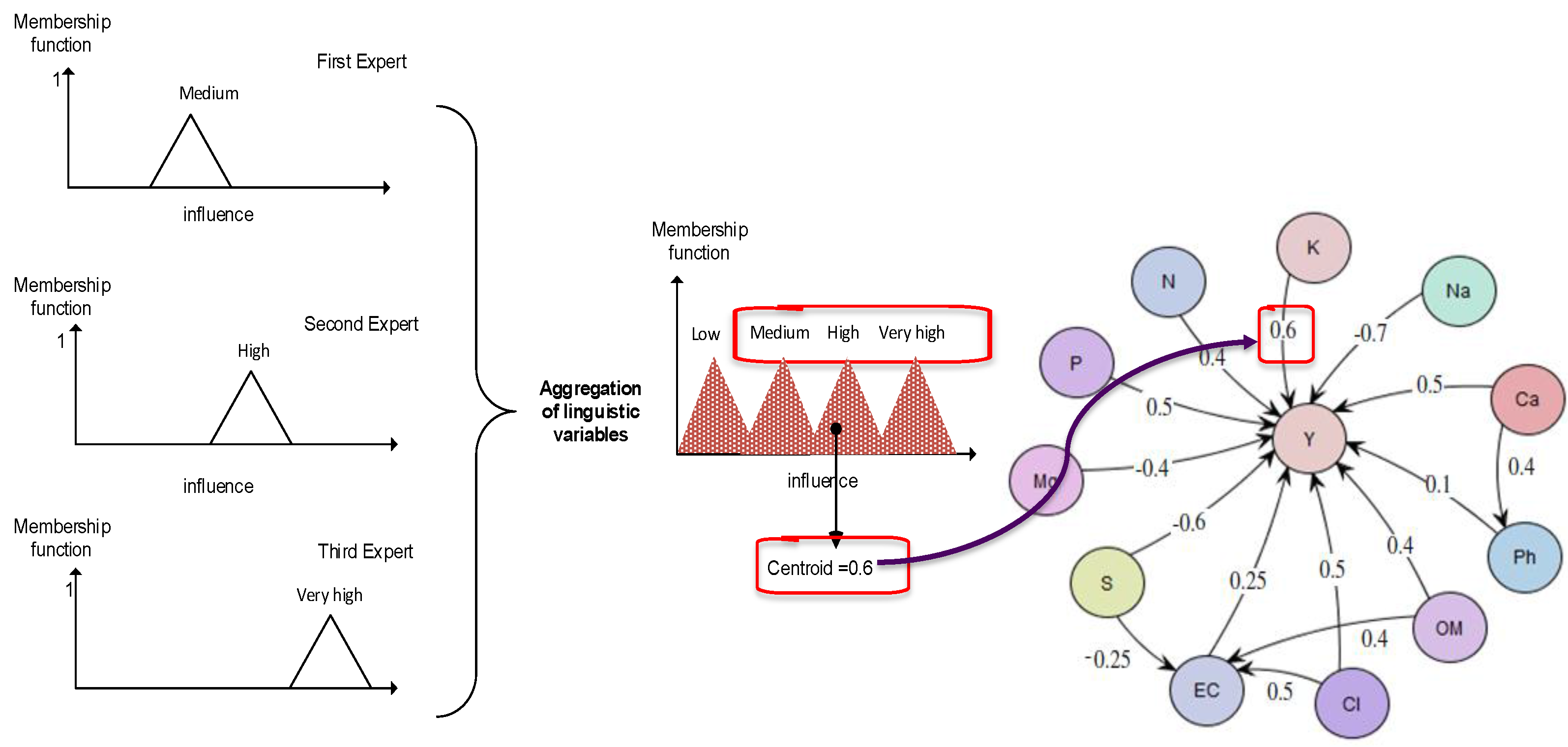
Figure 4.
Weight generation in SimulDRBFCM models.

Figure 5.
SimulDRBFCM inference algorithm.

Figure 6.
Influence fuzzy variable.

Figure 7.
With probability q = 0.95 (shaded area), the number of correct SimulDRBFCM simulations lies in an interval [] around the mean sentence score .
Figure 7.
With probability q = 0.95 (shaded area), the number of correct SimulDRBFCM simulations lies in an interval [] around the mean sentence score .
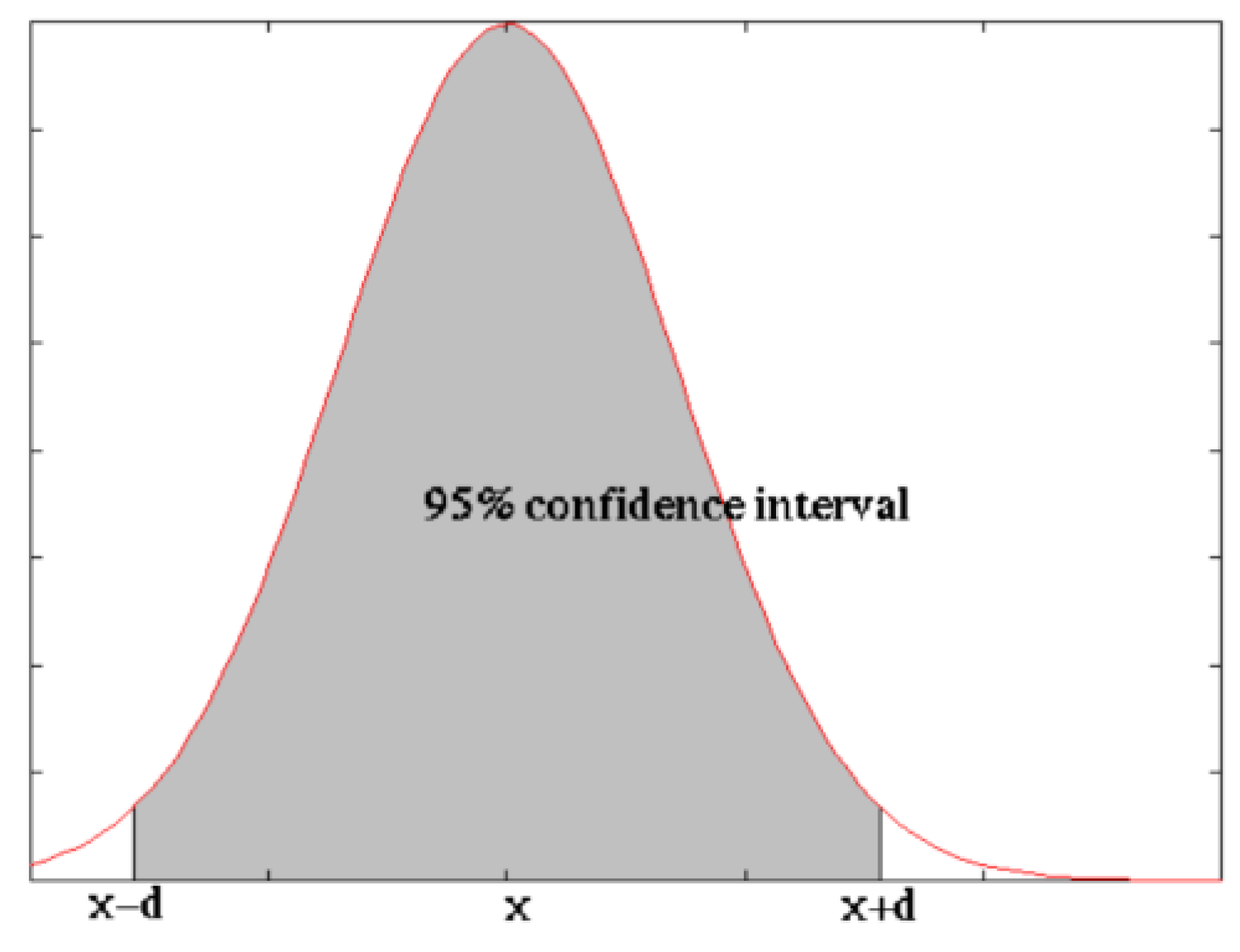
Figure 8.
Depiction and verification of the yield decrease percentage distribution produced on the set of the n = 2847 cases.
Figure 8.
Depiction and verification of the yield decrease percentage distribution produced on the set of the n = 2847 cases.


Table 1.
Soil parameters that affect cotton yield.
| Concept | Description |
|---|---|
| C1: EC | Soil shallow electrical conductivity Veris (mS/m) |
| C2: Mg | Magnesium (ppm) |
| C3: Ca | The measured calcium in the soil in depth 0–30 cm (ppm) |
| C4: Na | The measured Na (Sodium) in the soil in depth 0–30 cm (ppm) |
| C5: K | The measured Potassium in the soil in depth 0–30 cm (ppm) |
| C6: P | The measured Phosphorus in the soil in depth 0–30 cm (ppm) |
| C7: N | The measured NO3 in the soil profile of 0–30 cm (ppm) |
| C8: OM | The percent organic matter content in soil profile in depth 0–30 cm |
| C9: Ph | The pH of the soil in depth 0–30 cm |
| C10: S | The percent of the sand in the soil samples in depth 0–30 cm |
| C11: Cl | The percent of the clay in samples in depth 0–30 cm |
| C12: Y | Seed cotton yield from 1st picking measured by yield monitor (t ha−1) |
Table 2.
Membership function parameters for each of the FCM concepts.
| Concept | Membership Function | Concept | Membership Function |
|---|---|---|---|
| C1: (EC) | VL = TRAPE 0 0 7.5 15 | C7: (N) | VL = TRAPE 0 0 3 8 |
| L = TRAPE 10 18 18 25 | L = TRAPE 5 8 8 17.5 | ||
| M = TRAPE 25 28 28 35 | M = TRAPE 12 20 20 27.5 | ||
| H = TRAPE 30 38 38 45 | H = TRAPE 22 32 32 45 | ||
| VH = TRAPE 40 45 100 100 | VH = TRAPE 35 40 45 45 | ||
| C2: (Mg) | VL = TRAPE 0 0 60 120 | C8: (OM) | L = TRAPE 0 0 0.6 1.1 M = TRAPE 0.5 1.5 1.5 2.5 H = TRAPE 1.8 2.1 3 3 |
| L = TRAPE 60 140 140 240 | |||
| M = TRAPE 160 290 290 360 | |||
| H = TRAPE 300 500 500 1400 | |||
| VH = TRAPE 700 950 1400 1400 | |||
| C3: (Ca) | VL = TRAPE 0 0 455 1000 | C9: (Ph) | VL = TRAPE 0 0 4 5 |
| L = TRAPE 545 1273 1273 2000 | L = TRAPE 4 5 5 6 | ||
| M = TRAPE 1363 2455 2455 3000 | SL = TRAPE 5 6 6 7 | ||
| H = TRAPE 2637 3909 3909 5000 | M = TRAPE 6 7 7 8 | ||
| VH = TRAPE 4000 4380 5000 5000 | SH = TRAPE 7 8 8 9 | ||
| C4: (Na) | VL = TRAPE 0 0 26 59 | C10: (S) | L = TRAPE 0 0 15 30 M = TRAPE 20 45 45 70 H = TRAPE 60 75 75 90 VH = TRAPE 80 90 100 100 |
| L = TRAPE 32 70 70 123 | |||
| M = TRAPE 80 140 140 200 | |||
| H = TRAPE 156 250 250 600 | |||
| VH = TRAPE 350 450 600 600 | |||
| C5: (K) | VL = TRAPE 0 0 24 65 | C11: (Cl) | L = TRAPE 0 0 12.5 20 M = TRAPE 10 22.5 22.5 35 H = TRAPE 30 37.7 60 60 |
| L = TRAPE 30 81 81 135 | |||
| M = TRAPE 88 152 152 230 | |||
| H = TRAPE 190 275 275 600 | |||
| VH = TRAPE 300 470 600 600 | |||
| C6: (P) | VL = TRAPE 0 0 5 10 | C12: (Y) | L = TRAPE 0 0 2 3 H = TRAPE 2 3 6 6 |
| L = TRAPE 5 12.5 12.5 20 | |||
| M = TRAPE 12.5 22 22 31.5 | |||
| H = TRAPE 25 38 38 50 | |||
| VH = TRAPE 40 45 50 50 |
Table 3.
The different rule blocks for cotton yield links expressed in the modified FCL.
| Concept | If-Then Rules | Concept | If-Then Rules |
|---|---|---|---|
| C1:(EC) | IF EC IS VL THEN VAR IS PVL ON Y | C6:(P) | IF P IS VL THEN VAR IS PM ON Y IF P IS L THEN VAR IS PM ON Y IF P IS M THEN VAR IS PM ON Y IF P IS H THEN VAR IS PM ON Y IF P IS VH THEN VAR IS PM ON Y |
| IF EC IS M THEN VAR IS PL ON Y | |||
| IF EC IS H THEN VAR IS PM ON Y | |||
| IF EC IS H THEN VAR IS PH ON Y | |||
| IF EC IS VH THEN VAR IS PH ON Y | |||
| IF EC IS L THEN VAR IS PVL ON Y | |||
| C2:(Mg) | IF Mg IS VL THEN VAR IS NL ON Y IF Mg IS L THEN VAR IS NL ON Y IF Mg IS M THEN VAR IS NM ON Y IF Mg IS H THEN VAR IS NM ON Y IF Mg IS VH THEN VAR IS NM ON Y | C7:(N) | IF N IS VL THEN VAR IS PVL ON Y |
| IF N IS L THEN VAR IS PL ON Y | |||
| IF N IS M THEN VAR IS PL ON Y | |||
| IF N IS H THEN VAR IS PL ON Y | |||
| IF N IS VH THEN VAR IS PM ON Y | |||
| IF N IS VH THEN VAR IS PL ON Y | |||
| C3:(Ca) | IF Ca IS VL THEN VAR IS PM ON Y | C8:(OM) | IF OM IS L THEN VAR IS PL ON Y IF OM IS M THEN VAR IS PL ON Y IF OM IS H THEN VAR IS PM ON Y |
| IF Ca IS L THEN VAR IS PL ON Y | |||
| IF Ca IS M THEN VAR IS PM ON Y | |||
| IF Ca IS H THEN VAR IS PM ON Y | |||
| IF Ca IS VH THEN VAR IS PM ON Y | |||
| IF Ca IS VH THEN VAR IS PL ON Y | |||
| C4:(Na) | IF Na IS VL THEN VAR IS NVH ON Y IF Na IS VL THEN VAR IS NH ON Y IF Na IS L THEN VAR IS NM ON Y IF Na IS M THEN VAR IS NL ON Y IF Na IS H THEN VAR IS NH ON Y IF Na IS VH THEN VAR IS NH ON Y IF Na IS VH THEN VAR IS NVH ON Y | C9: (Ph) | IF Ph IS VL THEN VAR IS PVL ON Y |
| IF Ph IS VL THEN VAR IS PL ON Y | |||
| IF Ph IS L THEN VAR IS PVL ON Y | |||
| IF Ph IS SL THEN VAR IS PVL ON Y | |||
| IF Ph IS M THEN VAR IS PVL ON Y | |||
| IF Ph IS SH THEN VAR IS PVL ON Y | |||
| IF Ph IS H THEN VAR IS PVL ON Y | |||
| IF Ph IS H THEN VAR IS PL ON Y | |||
| IF Ph IS VH THEN VAR IS PVL ON Y | |||
| IF Ph IS VH THEN VAR IS PM ON Y | |||
| C5:(K) | IF K IS VL THEN VAR IS PVL ON Y | C10: (S) | IF S IS L THEN VAR IS NM ON Y |
| IF K IS L THEN VAR IS PVL ON Y | IF S IS L THEN VAR IS NH ON Y | ||
| IF K IS M THEN VAR IS PM ON Y | IF S IS M THEN VAR IS NM ON Y | ||
| IF K IS H THEN VAR IS PM ON Y | IF S IS M THEN VAR IS NL ON Y | ||
| IF K IS VH THEN VAR IS PM ON Y | IF S IS H THEN VAR IS NM ON Y | ||
| IF K IS VH THEN VAR IS PH ON Y | IF S IS VH THEN VAR IS NH ON Y | ||
| C11: (Cl) | IF Cl IS L THEN VAR IS PM ON Y | ||
| IF Cl IS M THEN VAR IS PM ON Y | |||
| IF Cl IS H THEN VAR IS PM ON Y |
Table 4.
FCM and SimulDRBFCM weights.
| Concept | Cotton Yield (Y) | |
|---|---|---|
| FCM | SimulDRBFCM a | |
| EC | 0.25 | 0.22 ± 2.0488 × 10⁻⁴ |
| Mg | −0.4 | −0.48 ± 4.27 × 10⁻² |
| Ca | 0.5 | 0.48 ± 3.15 × 10⁻² |
| Na | −0.7 | −0.7 ± 2.00 × 10⁻¹⁵ |
| K | 0.6 | 0.22 ± 1.88 × 10⁻⁴ |
| P | 0.5 | 0.49 ± 5.24 × 10⁻² |
| N | 0.4 | 0.35 ± 1.51 × 10⁻² |
| OM | 0.4 | 0.35 ± 8.23 × 10⁻³ |
| pH | 0.1 | 0.26 ± 2.37 × 10⁻² |
| S | −0.6 | −0.5 ± 7.07 × 10⁻¹⁶ |
| Cl | 0.5 | 0.5 ± 5.47 × 10⁻¹⁶ |
a Mean values shown with standard deviation.
Table 5.
Simulation results for the four scenarios (decrease by 2.5%, 5%, 7.5%, and 10%).
| ΔK (%) | ΔP (%) | ΔN (%) | Average Yield Decrease (%) | High to Low Yield Decrease (%) |
|---|---|---|---|---|
| Maximum Yield Decrease: 2.5% | ||||
| −10 | −10 | - | 2.55 | 1 |
| Maximum Yield Decrease: 5% | ||||
| - | −40 | - | 4.80 | 3 |
| - | −10 | −40 | 5.06 | 3 |
| - | - | −50 | 4.80 | 3 |
| −10 | −20 | −10 | 4.80 | 3 |
| −10 | −30 | - | 5.06 | 3 |
| −20 | - | −20 | 4.80 | 3 |
| −20 | −10 | −10 | 5.06 | 3 |
| Maximum Yield Decrease: 7.5% | ||||
| - | −50 | −10 | 7.19 | 6 |
| - | −40 | −20 | 6.92 | 5 |
| - | −10 | −60 | 7.19 | 6 |
| - | - | −70 | 6.92 | 5 |
| −10 | −30 | −20 | 7.19 | 6 |
| −10 | −20 | −30 | 6.92 | 5 |
| −20 | −10 | −30 | 7.19 | 6 |
| −20 | - | −40 | 6.92 | 5 |
| −30 | −20 | - | 6.92 | 5 |
| −40 | −10 | - | 7.19 | 6 |
| −40 | - | −10 | 6.92 | 5 |
| Maximum Yield Decrease: 10% | ||||
| - | −60 | −20 | 9.71 | 7 |
| - | −20 | −70 | 9.71 | 7 |
| - | −30 | −60 | 10.00 | 8 |
| - | −70 | −10 | 10.00 | 8 |
| −10 | - | −80 | 9.71 | 7 |
| −10 | −40 | −30 | 9.71 | 7 |
| −10 | −10 | −70 | 10.00 | 8 |
| −10 | −50 | −20 | 10.00 | 8 |
| −20 | −20 | −40 | 9.71 | 7 |
| −20 | −30 | −30 | 10.00 | 8 |
| −30 | - | −50 | 9.71 | 7 |
| −30 | −40 | - | 9.71 | 7 |
| −30 | −10 | −40 | 10.00 | 8 |
| −40 | −20 | −10 | 9.71 | 7 |
| −40 | −30 | - | 10.00 | 8 |
| −50 | - | −20 | 9.71 | 7 |
| −50 | −10 | −10 | 10.00 | 8 |
| −60 | −80 | −90 | 10.00 | 8 |
Table 6.
K, P, N, and Y values under the different scenarios.
| Scenario | MIN | MAX | MEAN | SDV a |
|---|---|---|---|---|
| 2.5% | ||||
| K | 0.207 | 0.4 | 0.279586 | 0.0634 |
| P | 11.832 | 20.01 | 15.83779 | 1.97 |
| N | 6.24 | 16.9 | 11.02034 | 3.36 |
| Y | 246.1704 | 249.721 | 248.1631 | 0.991 |
| 5% | ||||
| K | 0.161 | 0.51 | 0.291374 | 0.0861 |
| P | 10.353 | 23.72 | 15.85973 | 2.62 |
| N | 4.68 | 16.9 | 9.949553 | 3.06 |
| Y | 240.5466 | 249.8426 | 245.5901 | 2.51 |
| 7.5% | ||||
| K | 0.138 | 0.57 | 0.294396 | 0.0845 |
| P | 7.395 | 39.04 | 16.7129 | 5.65 |
| N | 2.34 | 26.3 | 9.433609 | 3.52 |
| Y | 233.8835 | 249.9708 | 243.5175 | 4.38 |
| 10% | ||||
| K | 0.092 | 0.57 | 0.29462 | 0.0901 |
| P | 4.437 | 39.04 | 16.01736 | 5.87 |
| N | 0.78 | 26.3 | 9.088008 | 4.11 |
| Y | 226.8011 | 249.9879 | 240.8015 | 5.97 |
a SDV: Standard Deviation.
Table 7.
Paired Samples Test (95% confidence interval).
| Paired Sample Names | Paired Differences | ||||||
|---|---|---|---|---|---|---|---|
| Mean | Std. Deviation | Std. Error Mean | 95% Confidence Interval of the Difference | t | |||
| Lower | Upper | ||||||
| Pair 1 | kdecr-yielddecr | −0.08693991 | 0.15064377 | 0.00282330 | −0.09247583 | −0.08140398 | −30.423 |
| Pair 2 | pdecr-yielddecr | −0.13095115 | 0.18151794 | 0.00340193 | −0.13762165 | −0.12428064 | −38.64 |
| Pair 3 | Ndecr-yielddecr | −0.19255686 | 0.22737567 | 0.00426138 | −0.20091556 | −0.18420415 | −45.56 |
Table 8.
Paired Samples Test (97% confidence interval).
| Paired Sample Names | Paired Differences | ||||||
|---|---|---|---|---|---|---|---|
| Mean | Std. Deviation | Std. Error Mean | 97% Confidence Interval of the Difference | t | |||
| Lower | Upper | ||||||
| Pair 1 | kdecr-yielddecr | −0.08693991 | 0.15064377 | 0.00282330 | −0.09247583 | −0.08140398 | −30.755 |
| Pair 2 | pdecr-yielddecr | −0.13095115 | 0.18151794 | 0.00340193 | −0.13762165 | −0.12428064 | −38.433 |
| Pair 3 | ndecr-yielddecr | −0.19255686 | 0.22737567 | 0.00426138 | −0.20091556 | −0.18420415 | −45.167 |
Table 9.
Paired Samples Test (99% confidence interval).
| Paired Sample Names | Paired Differences | ||||||
|---|---|---|---|---|---|---|---|
| Mean | Std. Deviation | Std. Error Mean | 99% Confidence Interval of the Difference | t | |||
| Lower | Upper | ||||||
| Pair 1 | kdecr-yielddecr | −0.08693991 | 0.15064377 | 0.00282330 | −0.09247583 | −0.08140398 | −30.794 |
| Pair 2 | pdecr-yielddecr | −0.13095115 | 0.18151794 | 0.00340193 | −0.13762165 | −0.12428064 | −38.493 |
| Pair 3 | ndecr-yielddecr | −0.19255686 | 0.22737567 | 0.00426138 | −0.20091556 | −0.18420415 | −45.187 |
Table 10.
Mann–Whitney U-Test Ranks.
| Match | N | Mean Rank | Sum of Ranks | |
|---|---|---|---|---|
| Yield-reduction | 1 | 17,624 | 11,102.63 | 1.96×10⁸ |
| 2 | 3071 | 6017.30 | 18,479,117.00 | |
| Total | 20,695 | |||
| K-reduction | 1 | 17,624 | 10,501.16 | 1.85×10⁸ |
| 2 | 3071 | 9469.03 | 29,079,397.00 | |
| Total | 20,695 | |||
| P-reduction | 1 | 17,624 | 10,273.80 | 1.81×10⁸ |
| 2 | 3071 | 10,773.84 | 33,086,475.00 | |
| Total | 20,695 | |||
| N-reduction | 1 | 17,624 | 10,348.00 | 1.82×10⁸ |
| 2 | 3,071 | 10,348.00 | 31,778,708.00 | |
| Total | 20,695 |
Table 11.
Mann–Whitney U-Test Statistics a.
| Yield-reduction | K-reduction | P-reduction | N-reduction | |
|---|---|---|---|---|
| Mann–Whitney U | 1.376×10⁷ | 2.436×10⁷ | 2.575×10⁷ | 2.706×10⁷ |
| Wilcoxon W | 1.848×10⁷ | 2.908×10⁷ | 1.811××108 | 3.178×10⁷ |
| Z | −43.531 | −8.863 | −4.83 | 0.000 |
| Asymp. Sig. (two-tailed) | 0.000 | 0.000 | 0.000 | 1.000 |
a Grouping Variable: Match.
© 2017 by the authors. Licensee MDPI, Basel, Switzerland. This article is an open access article distributed under the terms and conditions of the Creative Commons Attribution (CC BY) license (http://creativecommons.org/licenses/by/4.0/).
Share and Cite
MDPI and ACS Style
Mourhir, A.; Papageorgiou, E.I.; Kokkinos, K.; Rachidi, T. Exploring Precision Farming Scenarios Using Fuzzy Cognitive Maps. Sustainability 2017, 9, 1241. https://doi.org/10.3390/su9071241
AMA Style
Mourhir A, Papageorgiou EI, Kokkinos K, Rachidi T. Exploring Precision Farming Scenarios Using Fuzzy Cognitive Maps. Sustainability. 2017; 9(7):1241. https://doi.org/10.3390/su9071241
Chicago/Turabian StyleMourhir, Asmaa, Elpiniki I. Papageorgiou, Konstantinos Kokkinos, and Tajjeeddine Rachidi. 2017. "Exploring Precision Farming Scenarios Using Fuzzy Cognitive Maps" Sustainability 9, no. 7: 1241. https://doi.org/10.3390/su9071241
Note that from the first issue of 2016, this journal uses article numbers instead of page numbers. See further details here.