Optimal Environmental Regulation Intensity of Manufacturing Technology Innovation in View of Pollution Heterogeneity

1
School of Management, Shanghai University, Shanghai 200444, China
2
School of Economics & Management, Tongji University, Shanghai 200444, China
*
Author to whom correspondence should be addressed.
Sustainability 2017, 9(7), 1240; https://doi.org/10.3390/su9071240
Submission received: 10 June 2017
/
Revised: 6 July 2017
/
Accepted: 11 July 2017
/
Published: 15 July 2017
(This article belongs to the Section Economic and Business Aspects of Sustainability)
Abstract
:Based on panel data of 28 manufacturing industries sectors in 2005–2015 years, this paper first estimated the level of 28 manufacturing industries sectors technological progress, and then, using panel threshold technology, calculated the impact of three environmental regulation change rates on technological progress change rate to analyze the relationship between environmental regulations and technology innovation. The results show that: (1) The influence of the change rates of waste gas, wastewater and solid waste’s environmental regulation intensity towards the change rate of production technological progress has two thresholds. Only the proper change rate of environmental regulation intensity can lead to a desired change rate of production technological progress. However, there are differences in the thresholds of the change rates of three kinds of environmental regulation intensities, and the optimal change rates of waste gas, wastewater and waste solid are 15.07%–55.31%, 17.06%–38.02% and 33.12%–47.99%, respectively. (2) In the change rates of waste gas, wastewater and waste solid’s environmental regulation intensity, there are 8, 10 and 3 industries at a reasonable level, respectively, while others industries are below or above the reasonable level and unable to stimulate technical and management innovation in enterprises. Hence, to achieve a win-win situation between environmental protection and production technological progress, different environmental regulation intensities should be planned according to different pollutants in various manufacturing industries.
1. Introduction
Porter Hypothesis [1] argues that reasonable environmental regulation can give the manufacturing industry a signal that inefficient resource allocation exists and that technology needs to be improved, triggering an innovation compensation effect, which can not only offset the compliance costs, but also increase manufacturing productivity and competitiveness. This hypothesis provides a theoretical support for the win-win situation of environmental regulation and economic growth, and the basic premise of this theory requires a significant innovation compensation effect. To verify whether the innovation compensation effect is sufficient to support the reality of Porter Hypothesis, many scholars have carried out a great deal of research on environmental regulation issues [2,3,4,5,6,7,8,9].
With regard to the effect of environmental regulations on manufacturing pollution control technology progress, scholars generally agree that environmental regulation can bring significant positive effects on pollution control technology progress [2]. In general, the incentive effect of sewage tax and auction of pollution permits on manufacturing industry pollution control technology progress is better than that of tradable emission permit [3].
However, scholars’ views are not unified regarding the effect of environmental regulation on manufacturing industry technological progress. The differing viewpoints can be divided into three categories: promote theory, suppression theory and uncertainty theory.
In the first view, scholars believe that environmental regulations can increase technology innovation level. This view supports the Porter hypothesis strongly. For example, Bhatnager & Cohen [4] studied the effect of environmental regulation on industrial technology innovation in 146 American manufacturing industries from 1983 to 1992, and the results demonstrated that there is a significant positive correlation between pollution abatement cost and environmental patent filings.Whitford & Tucker [5] found that, for every 1% increase in pollution abatement costs, Research and Development (R&D) expenditure will increase 0.15%, which means that there is a positive correlation between R&D expenditure and pollution abatement cost. Carrion and Innes [6] used 127 American manufacturers from 1989 to 2002 as research sample to explore the relationship between enterprise pollution emissions and environmental protection technology patents, and found that environmental regulation policy can incentivize industry to innovate. Horbach [7] found that environmental regulation, environmental management tools and the changes organization culture in Germany are all conducive to environmental protection and innovation. Li and Wang [8,9] tested Chinese environmental regulation and technological innovation relationship from 1994 to 2009, and the results showed that environmental regulation could spur overall innovation while ameliorating environmental pollution.
The second view is suppression, and researchers who hold this view claim that environmental regulation hinders technological innovation, i.e. negative Porter hypothesis. For instance, Wagner [10] took German manufacturing as an example, and empirically analyzed the relationships among environmental management, environmental innovation and patent application. The results showed that the level of environmental management system implementation and a company’s overall patenting activity are negatively related. Chintrakarn [11] used SFA model to evaluate the influence of environmental regulation on the manufacturing sector inefficiency in 48 American states. The results showed that stringent environmental regulation and US manufacturing technical inefficiency have a significant positive correlation. Acemoglu [12] found that environmental regulation leads to production costs rising, thus hindering technological innovation.
The third view is uncertainty, and scholars who hold this view claim that there is no obvious relationship between environmental regulation and technological innovation or economic performance. For example, Alpaye and Buccola [13] took the American and Mexican food industry as the research object to analyze the effects of environmental regulation on productivity from 1971 to 1994. The results indicated that the effect of environmental regulation on the food industry productivity in the United States is negative, while the same impact in Mexico is positive. Domazlicky [14] analyzed the operation cost and technical efficiency of chemical industry data from 1988 to 1993 and found there is no evidence showing that environmental regulation will inevitably lead to industrial technical efficiency decline. Kneller [15] made an empirical analysis of the effect of environmental regulation on technological innovation and found the effect is not obvious.
From the above literature review, we found that previous studies mainly examined the impact of environmental regulation on two kinds of technological progress from the time dimension, and considered that the two will be consistent with the U type evolution trajectory. This U type trajectory depends on the contrast of the positive effects (innovation compensation) and negative effects (followed cost) brought by environmental regulation, and the positive effects of innovation compensation often lag behind the negative effects of cost compliance. Analyzing the dynamic relationship between environmental regulation and technological advances from time dimensions is often unsatisfactory, which forces scholars to think about the applicability of Porter Hypothesis. Scholars have found that other factors, such as the rationality of environmental regulation policy [3], environmental regulation intensity [16], human capital level [17], enterprise technical level [18], enterprise market forces [19] and economic development [20], might affect the relationship between environmental regulation and technological progress. However, the existing research focusing on environmental regulation intensity rationality is limited.
Although Nagurney [21] and Bréchet et al. [22] explored the rationality of environmental regulation policies, such as emission rights and carbon taxes, they mainly analyzed from the perspective of economic growth and pollution control. The literature exploring the reasonable interval of environmental regulation intensity from the perspective of production technology progress is rare. As Parry [23] pointed out, while it is expected that environmental regulation will lead to technological progress that will change the future emission reduction costs and production levels, the problem is that predicting which environmental regulation will evoke technical progress is difficult, which leads to optimal environmental regulation intensity being difficult to measure. However, if we assume that the same intensity of environmental regulation can lead to the same rate of technological progress based on the control of relevant factors, we can analyze the reasonable intensity of environmental regulation interval from technological progress perspective. Based on this hypothesis, in the analysis of environmental regulation level value, some scholars believe that environmental regulation intensity will cause a nonlinear “U” type trajectory on production technological progress and pollution control technology progress [16,20], while others think the influence trajectory should be the type of “∽” [24].
It is reasonable to study the nonlinear effect of environmental regulation on technological progress from the intensity dimension. Becher [16] also pointed out why different environmental regulation intensities would cause different effects on production technological progress. Based on the nonlinear hypothesis on the intensity dimension, it is possible to answer the question of why some environmental regulations do not lead to the ideal innovation compensation effect. However, several existing studies have used the level values of environmental regulation intensity to participate in the measurement regression when they tested the nonlinear hypothesis of intensity dimension. This implies an important assumption mentioned above: the endogenous inflection point of each economy in environmental regulation intensity is the same; that is, when it reaches a certain level, it will bring about the same impact on production technological progress. This hypothesis ignores the differences between regions and sectors, such as the differences of endogenous inflections in highly polluting economies and low-polluting economies. Therefore, we believe that using environmental regulation intensity in regression analysis is questionable. The environmental regulation intensity should be dynamically adjusted, and cannot be confined to a particular level, which requires environmental regulation intensity to continually improve to ensure its continuous incentive for the level of production technology.
To enrich the relevant research, this paper uses panel technology threshold to study the nonlinear relationship between environmental regulation intensity and technological innovation in manufacturing based on Chinese manufacturing sub-sector panel data. We analyze the reasonable range of environmental regulation intensity from the perspective of technological advances, which can help us understand the changing trends of environmental regulation intensity more comprehensively, and understand why some environmental regulation failed to bring ideal innovation compensatory effects. Therefore, this study provides valuable reference for China’s scientific development of environmental regulations and policies. The main contributions of this study include: (1) using the change rate of environmental regulation intensity and production technological advancements as core variables; and (2) determining the change range of optimal waste gas, wastewater and waste solid regulation intensity base on pollutant heterogeneity.
The rest of the paper is organized as follows. In Section 2, we present our model and describe our empirical strategy, including data description and estimation strategies. Section 3 presents an empirical research and analyzes the empirical results. In Section 4, the research result is discussed. Conclusions are given in Section 5.
2. Model Setting and Data Description
2.1. Model Setting
DEA and SFA are the two methods that can be used to measure the rate of production technology of China’s industrial sub-sectors, both having their own advantages and disadvantages. DEA model does not need to recognize the stochastic factors, but requires a specific parameter regression. SFA method can identify random factors, but often falls into the problem of parameter regression. However, a large number of studies have confirmed that the two results are highly related. In this paper, we use the DEA-based Malmquist productivity index for analysis, and further take one of its decomposition variables (technological progress changes) as a technological progress indicator; the specific construction steps are described later.
2.1.1. Malmquist-DEA
In the DEA methodology, first, efficiency is defined as a ratio of weighted sum of outputs to a weighted sum of inputs, where the weight structure is calculated by means of mathematical programming, and constant returns to scale (CRS) are assumed. Later, Banker, Charnes and Cooper developed a model with variable returns to scale (VRS), and Tone proposed a simple method for deciding the local returns-to-scale characteristics of DMUs (Decision Making Units) in Data Envelopment Analysis. From the relevant literature, we found that data envelopment analysis (DEA) method has been used widely to measure the rate of technological progress and obtained fruitful research results [25,26]. The advantage of DEA is that the production function can be neglected and multi-index output can be measured. However, the drawback of DEA is that the production frontier should be set in advance and the efficiency value obtained from the calculations is the relative efficiency value. To improve DEA method, researchers have established a plurality of DEA models and efficiency measurement indicator frameworks from different perspectives. The existing DEA methods are mainly divided into two categories: (1) the technical efficiency measure model in a static perspective; and (2) the technical efficiency measure model in a dynamic perspective. In the static model, the most notable assumption is that all decision making units are in the same technical conditions. The main measure models include CCR (Charnes–Cooper–Rhodes) and BCC (Banker–Charnes–Cooper), etc. [27]. In the dynamic model, the technical level of decision making units changes with time series. In this study, we make technical efficiency measures in the case of time-series change to observe the relationship between production frontier and the time sequence variation. The results obtained from this dynamic technical efficiency measure model can be called total factor productivity changes, and the main models are VRS-TE and Malmquist-DEA. The VRS-TE model, also called “multi stage variable scale return” algorithm, was proposed by Coelli [28]. It is characterized by the relevant elements and scale returns of the decision making unit change with the time series. The Malmquist DEA model is proposed by Fare [29]; its basic idea is to examine productivity changes based on traditional DEA model. The result thus obtained was named Malmquist-TFPch.
Technological progress is a cumulative process: the preliminary technical foundation and investment will have a certain impact on technological advances later. Thus, using a static measure model will produce bias. At the same time, because the technological progress is affected by many factors, endogenous factors inevitably exist in the model due to the limitations of data sources and variable omissions. Thus, we use the Malmquist-DEA method in this research. Furthermore, we will take one of its decomposition variables (change of technological progress) as an indicator of production technology progress. The DEA-Malmquist index method has the following advantages: (1) it does not need the element price information; (2) panel data analysis among multiple objects are applied; and (3) TFP can be decomposed into the product of technical progress and technical efficiency change, and technical efficiency can be further decomposed into the product of pure product efficiency and scale efficiency.
Motivated by the study of Fare et al. [29], the specific construction steps of the model are as follows.
● Step 1: Define Malmquist productivity index on the basis of distance function:
Taking the technical level T (t) in t period and technical level T (t + 1) in (t + 1) period as the reference, the output-based Malmquist index can be expressed as:
and
where and represent the input and output vectors of t period and (t + 1) period, respectively; and and represent the distance functions of t period and (t + 1) period, respectively.
● Step 2: Calculate Malmquist index
To avoid possible differences produced by random selection of period, the geometric mean of Equations (1) and (2) is used as a measure of the Malmquist index from t period to (t + 1) period [30,31]:
When the index is greater than 1, it indicates that TFP is growing from t period to t + 1 period, and vice versa.
● Step3: Decompose Equation (3)
Under the assumption that scale of returns is constant, the above equation can be divided into two items: technical changes and technological efficiency changes. That is:
Using linear programming method with constant scale returns in DEA to calculate the value of each distance function d (°), we can get the Malmquist index, TFP.
The core concept of the DEA approach is the production decision unit. An important prerequisite for using DEA-Malmquist index is that the number of decision units should not be too small: it requires at least two times the number of model variables. Therefore, based on the data used in this study, which drew from 28 industrial outputs in 2005–2015, this method can expand the decision making unit and avoid unstable calculation results because of the sparse data. However, it is worth noting that this method will reduce the calculation period by S−1 cycles. Malmquist-DEA method can measure the change of technology efficiency. To measure the technical efficiency and its change more accurately, we also introduce Boot-strap correction technology in this paper for the estimation of nonparametric distance function.
2.1.2. Panel Threshold Regression Technique
We need to build econometric models to verify the nonlinear relationship between the environmental regulation intensity and production technological advances. For the measurement of this nonlinear relationship, scholars usually choose classic quadratic curve analysis methods used in environmental Kuznets curve (EKC). EKC was proposed by Grossman and Krueger [32]. In 1991, Grossman and Krueger found that there has an inverted U-shaped relationship between environmental pollution and economic development. It is called EKC because it resembles the inverted U-curve relationship between income disparity and economic growth described by Kuznets curve. However, there are two significant deficiencies in the EKC method: the independent variable level items and squared term is strongly correlated, and both sides of “U” or inverted “U” shaped inflection points must follow a symmetric distribution.
To avoid these shortcomings, this article uses panel threshold regression techniques to analyze the nonlinear relationship between environmental regulation intensity and production technological progress. The panel threshold regression model, proposed by Hansen [33], has three key points: (1) verify the existence of threshold effects and find the threshold value; (2) test the significant of threshold to determine the thresholds number; and (3) determine the model form according to threshold test results and estimate the model parameter. The model can not only estimate the threshold value, but can also allow the threshold and threshold effect be subjected to a series of estimates and significance tests. In this study, we use the environment regulation intensity change rate and the production technological progress change rate to make panel threshold regression. First, we use panel threshold technique to estimate the specific coefficient values and corresponding significance level of the core argument on both sides of the threshold. If there is a threshold level τ of environmental regulation intensity change rate, then its effect on the rate of production of technological progress changes is significantly different on the different sides of the threshold. Assume dummy variable Dit satisfies:
Based on this, we can establish the following panel threshold model:
where i represents the industry, t represents the year, Rate T is technological progress change rate and Rate ER is environmental regulations strength change rate. Considering the lagged effects of the indicator, this paper inspects one-year lag. In addition, RAV, RCP, LP and Ownstr are control variables, representing rate of industrial value added, rate of cost profit, labor productivity and ownership structure, respectively. β is the parameter to be estimated; η is the individual effect; and u is a random error.
2.2. Description of Data and Variable
In this paper, the category of manufacturing in China Statistical Yearbook is used as the classification standard of manufacturing industry. The data used in research are all derived from China Statistical Yearbook (2005–2015), China Industrial Statistical Yearbook (2005–2015) and China environmental Statistical Yearbook (2005–2015) [34].
In calculating the technological progress rate, total industrial output value of 28 industries from 2005 to 2015 is used to represent desired outputs. These basic data are obtained from China Statistical Yearbook [34] and converted into constant 1995 prices, in accordance with sub-industry producer price index. Labor input uses average number of employees in manufacturing industries in 2005–2015 to calculate, the data can obtain from China Statistical Yearbook [34]. Capital investment uses industries’ capital stock of each year to calculate. Capital stock is an important input variable in productivity research but we must estimate it, as China Statistical Yearbook did not provide details on capital stock data. This paper uses the perpetual inventory method to estimate the industry capital stock during 2005–2015 based on data from China Statistical Yearbook [34]. Capital stock calculation depends on the solution of three issues: determining the capital stock in the base year, depreciation rate, and the amount of investment at constant prices for the year. We take the capital stock of 1980 as the base year capital stock in accordance with Chen’s research [35] and calculate depreciation rate based on the data of depreciation and fixed assets from China Statistical Yearbook and China Industrial Statistics Yearbook [34]. Then, calculating the investment amount for each year, we use the difference between the original values to construct an investment sequence and convert it into constant 1995 prices according to the investment goods price index. Finally, we obtain the annual capital stock data of various industries from 2005 to 2015 according to the formula for perpetual inventory method proposed by Lei [36].
There is no fixed pattern of government intervention and no independent regulatory tool in real environmental regulation practice, which brings a great deal of difficulty to calculating the environmental regulation intensity. The existing literature mainly has the following several methods: used the number of environmental regulation laws and policies to calculate [20], used sewage fee income to calculate [24], used the proportion of pollution control investments accounted for the total cost or value to calculate [37,38],and used per capita GDP to calculate [39]. Due to the differences in the nature of different manufacturing industries and emission intensity of different pollutants, we selected the output capacity change rate of pollutants per unit as an indirect measure index of the environmental regulation intensity based on measuring method of pollution reduction effect [40]. The specific equation is:
where Y is output, and W is the net emissions of waste gas, wastewater and waste solid. This formula can link the pollutant emissions with environmental regulation intensity in different manufacturing industries: the larger the economic output of unit pollutants, the stronger the environmental regulation intensity. On the contrary, it indicates weaker environmental regulation intensity. Taking the large differences of the three pollutants and their different tendencies of environmental regulation into account, we calculate the change rate of waste gas environmental regulation intensity (Rate ER Gas), the change rate of wastewater environmental regulation intensity (Rate ER Water) and the change rate of waste solid environmental regulation intensity (Rate ER Solid) to measure environmental regulation intensity [38,41].
In calculating control variables, the ratio of industrial added value and industrial output in the same period are used to measure the rate of Industrial Added Value (RAV), which reflects the beneficial characteristics of industry intermediate consumption. The ratio of industry profits to industry cost in a given period is used to measure rate of cost profit (RCP), which reflects the economic benefits of lowering industry production costs. The ratio of industrial added value and the average number of employees are used to measure labor productivity (LP), which reflects the production technology level, management level, workers technical proficiency and labor enthusiasm comprehensively. The ratio of assets of state-owned and state-holding industries to total industrial enterprises above designated size is used to measure ownership structure (Ownstr) [11,42,43,44].
3. Empirical Results and Analysis
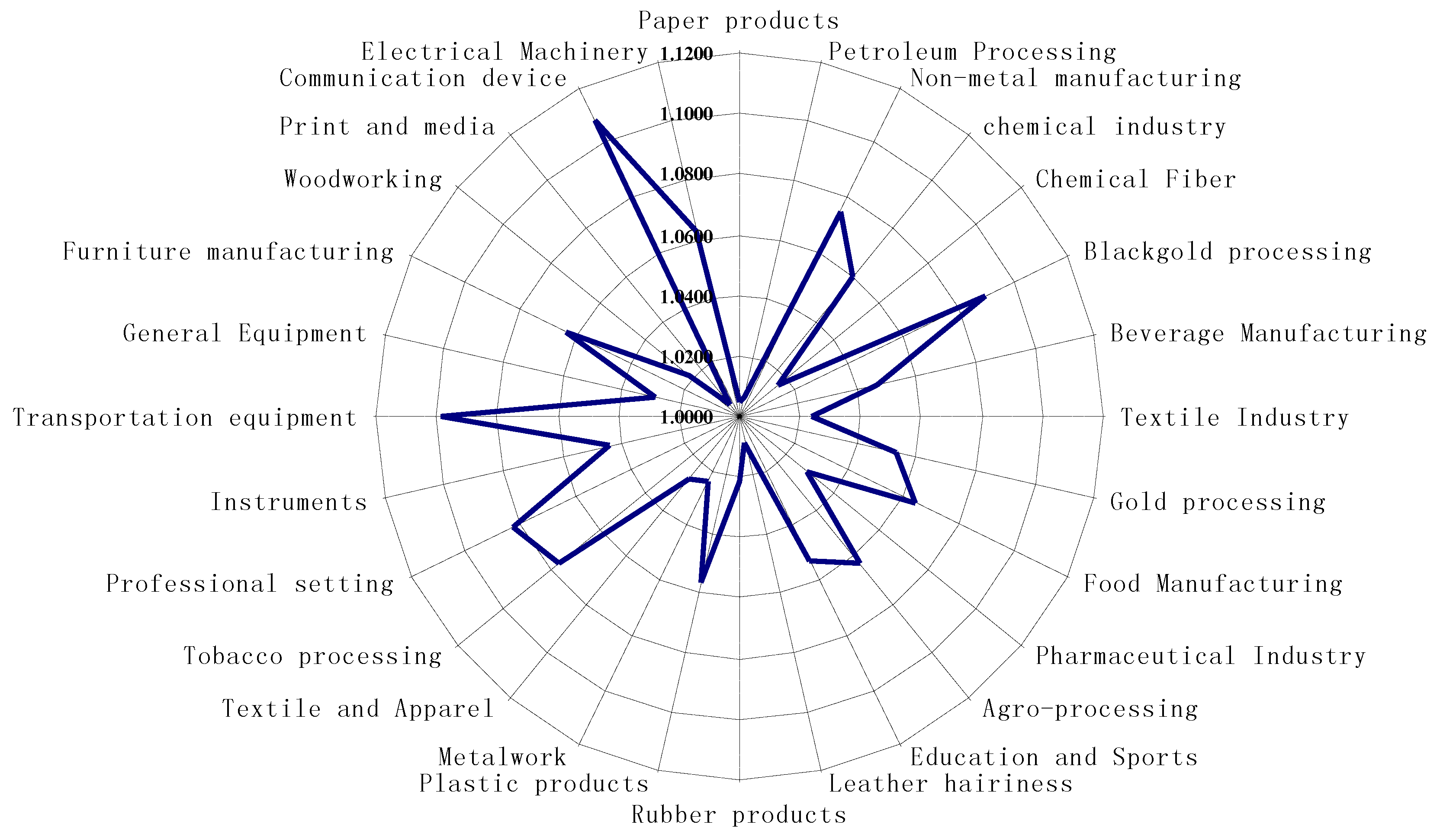
In this paper, we use software DEAP2.1 to calculate DEA Malmquist Malmquist-DEA productivity index of 28 manufacturing industries from 2005 to 2015. The result is shown in Figure 1. It can be observed that the annual average advance rate of technological progress of all 28 manufacturing industries is greater than 1, and the mean is 1.085. Although each manufacturing industry has made certain technical progress, there is a big difference between their technological progress rates. For example, the average annual technological progress rate of communication device industry (0.173) is 38.44 times the progress rate of paper products (0.0045).
To determine the threshold number, we estimate the linear model, a single threshold model, two-threshold model and three-threshold model in turn, set the sampling frequency as 1000, and use the Bootstrap method to calculate the F statistic and p value. The results are shown in Table 1. In Table 1, we can see that the change rates of waste gas regulation intensity, wastewater regulation intensity and waste solid regulation intensity all reject the linear model at 1% significance level, and are subject to double threshold model at the significant level of 10%. However, all three variables do not pass the significant test of three-threshold model. Therefore, we can judge that all three environmental regulation intensity change rate indicators have two thresholds.
Table 2 reports the threshold regression results of three kinds of environmental regulation intensity change rates on production technology progress rate. Based on Table 2, we can obtain two threshold values for each kind of environmental regulation intensity change rate: the threshold values of waste gas regulations intensity change rate are 0.1507 and 0.5531; the threshold values of wastewater regulation intensity change rate are 0.1706 and 0.3802; and the threshold values of solid waste environmental regulation threshold intensity change rate are 0.3312 and 0.4799. Then, the threshold regression of the three environment regulation intensity change rates to the technological progress changes rate is performed, as shown in Table 2.
We can see in Table 2 that, when the change rate of waste gas regulation intensity is less than 15.07%, a 1% increase will bring −0.0098% negative impact to the technological progress. When the change rate of waste gas regulation intensity is located at interval 15.07%–55.31%, 1% increase will bring 0.1295% significant positive impact to the technology progress. When the change rate of waste gas regulation intensity greater than 55.31%, the previously positive role in promoting technology progress will change to non-significant negative inhibition. Therefore, with the change rate of waste gas regulation intensity from small to large, the change path of production technology progress rate will show “∽” type.
When the change rate of wastewater regulation intensity is less than 17.06%, it will bring non-significant positive impact to the technological progress; when the change rate of wastewater regulation intensity located from 17.06% to 38.02%, it will bring significant positive impact to the technology progress but the impact effect is slightly less than the waste gas impact effect at the corresponding interval; and when the change rate of wastewater regulation intensity greater than 38.02%, it will bring significant negative inhibition to the technology progress, although the impact coefficient is only −0.0713. Thus, the impact of waste gas regulation intensity change rate on the technology progress change rate shows inverted “U” shape.
For the regression of waste solid regulation intensity change rate, we found that the variable on both sides of the two thresholds are positive, indicating that, as the variable value increases, it always brings a positive role in promoting production technology progress. However, this positive role passes significant test only when the waste solid regulation intensity change rate s located in the interval 33.12%–47.99%.
From the control variable analysis results we can know that, although the improvement of RAV and RCP have a positive role in promoting the dependent variable, the impact did not pass the significance test because RAV and RCP can not only bring positive impact but also negative impact to technology progress: the positive impact comes from the increase of potential research investment, and the negative impact comes from monopoly research inert under the high value and high profits background. Improved LP have a significant positive impact to the dependent variable, indicating that workers technical proficiency and enthusiasm can improve technological innovation efficiency and are always the key to enterprise sustainable development. Moderate increase of the Ownstr will bring significant positive role in promoting the technological progress change rate. This indicates that technological progress in the state-owned and state holding enterprises is relatively faster than the foreign-funded enterprises and private enterprises, which reflects the backbone of state-owned enterprises in scientific innovation.
Moderate environmental regulation intensity can lead to a good level of technology progress; too high will lead to excessive heavy compliance costs, while too low will make regulation less of an incentive and reduce the green effect throughout the manufacturing process. Thus, we should decrease or increase regulation intensity to a reasonable level in practice. Thus, what level of environmental regulation intensity situation of the 28 Chinese manufacturing industries will exactly be in 2005–2015 years? Equation (7) was used to calculate the environmental regulation intensity of the three wastes, compare the calculation result with the three wastes threshold value, and get the environmental regulation intensity level of each industry. The results are shown in Table 3. We can know that, only beverage manufacturing, textile, pharmaceutical industry, agro-processing, education and sports, textiles, tobacco processing and transportation equipment have a reasonable waste gas regulation intensity level. Other industries do not meet the optimal level, wherein the regulation intensity of paper products, petroleum processing, non-gold manufacturing and 14 other industries are relatively low, while regulation intensity of special equipment, general equipment and six other industries is relatively high. On the intensity of wastewater regulation, 10 industries including chemical fiber and black gold processing industry have a reasonable level, the regulation intensity 13 industries is relatively low, and the regulation intensity of five industries is relatively high. Regarding the intensity of waste solid regulation, only non-metal manufacturing, beverage manufacturing and tobacco processing industries are reasonable; paper products, petroleum processing and 17 other industries’ regulation intensities are relatively low; and special equipment, electrical machinery and four other sectors are relatively high.
4. Discussion
Based on the panel data in 2005–2015 for manufacturing industries, this article estimated the level of 28 manufacturing industries technological progress, and then analyzed the impact of three kinds of environmental regulation change rates on technological progress change rate. It was found that the effect of the regulation intensity change rate of waste gas, wastewater and waste solid to technological progress have two threshold effect, and their optimal intervals of regulation intensity change rate were 15.07%–55.31%, 17.06%–38.02% and 33.12%–47.99%, respectively. Different from previous studies [5,6,7], this paper considers the pollution heterogeneity in empirical research and uses the environmental regulation intensity change rate to carry out regression analyses. These help us to understand how to formulate different environmental regulation intensities corresponding to different pollutants.
These results explain why the current scholars failed to reach unity on the relationship between environmental regulation intensity and production technology progress. If located at the reasonable endogenous destined threshold, environmental regulation intensity and production technology progress will show a positive correlation; otherwise, environmental regulation intensity and production technology progress will show a negative or no significant positive correlation.
From the related empirical results, the level of economic development is still the main factor affecting technological innovation everywhere: only in a country or region achieving a certain economic scale, strict environmental regulation is effective. We did not considerate the economic factor seriously, which may be the limitation of this study.
5. Conclusions
In this research, to figure out why some environmental regulation failed to illicit ideal innovation compensatory effects, we used panel technology threshold to analyze the nonlinear relationship between three kinds of environmental regulation intensity and technological innovation in manufacturing based on Chinese manufacturing sub-sector panel data from 2005 to 2015. According to the result, we found that, to achieve a win-win situation between environmental protection and production technological progress, different environmental regulation intensities should be used according to different pollutants of various manufacturing industries. Furthermore, we will perform a deeper study to analyze the nonlinear relationship between environmental regulation intensity and technological innovation, considering more influencing factors in the future.
Based on the above research, the following policy recommendations can be given.
First, the government should establish the optimal environmental regulation intensity in advance considering differences between industries and pollutants. Reasonable intensity of environmental regulation can provide continuous incentive for technology innovation and efficiency improvement of heavy pollution industry. When the environmental regulation intensity is too high, it cannot achieve the related technological innovation activities and achieve economic and environmental win-win situation, as described in the Porter Hypothesis. This will lead to low efficiency, and small or medium sized enterprises will prefer to develop at the expense of the environment, and weaken environmental regulation strength due to the lower cost, often overlooked by the enterprises, thus it cannot stimulate enterprise technological innovation and produce green effect.
Second, the government should adjust environmental regulation intensity level dynamically. In the case of asymmetric information, governments developing environmental regulation standards will overestimate or underestimate the real emissions compliance costs. Thus, the environmental regulation intensity cannot play a binding effect. Only if the government monitors the effectiveness and implementation of timely innovation, and focuses on revising the intensity of environmental regulation to a reasonable level, will the regulation standards continue to be business constraints and incentivize innovation.
Third, the government should grasp the technique of environmental regulation. The impact of environmental regulations on technological innovations and technological advance depends not only on environmental regulation degree but also on the environmental regulation tools. The relevant theory of environmental regulation tools claim that “controlled” environmental regulation tools, such as environmental standards, emission allowances, product bans and other regulatory instruments, will result in increased business costs and productivity decline and lack of adequate incentives for green technology R&D. However, “incentive” environmental regulation tools, such as emissions trading, environmental subsidies and other flexible market-based instruments, can help enterprise to find better means to reduce pollution and provide ongoing incentives to improve enterprise efficiency and technological innovation. Therefore, to improve the green total factor productivity of Chinese manufacturing and achieve the environmental benefits and economic development win-win situation, the Government should not only develop an appropriate level of environmental regulation in accordance with industrial properties and development characteristics, but also change environmental regulation from the control model, to incentive-based policy so that companies develop green technology and manage innovation comprehensively.
Acknowledgments
The authors are very grateful to the editor and reviewers for their insightful and constructive comments and suggestions which are very helpful in improving the quality of the paper. This work was partially supported by China Postdoctoral Science Foundation (No.2016M601565), Planning of Shanghai soft science (No.17692103800),the National Natural Science Foundation of China (Nos. 71671125 and 71402090) , and Anhui social science innovation development research project (No.2016CX070).
Author Contributions
All three authors contributed equally to gathering information, writing the manuscript, editing the manuscript and preparation of the figures.
Conflicts of Interest
The authors declare no conflict of interest.
References
- Porter, M.E. America’s green strategy. Sci. Am. 1991, 13, 264–268. [Google Scholar]
- Brunnermeier, S.B.; Cohen, M.A. Determinants of environmental innovation in US manufacturing industries. J. Environ. Econ. Manag. 2003, 45, 278–293. [Google Scholar] [CrossRef]
- Xu, S.C.; He, Z.X. The effect of environmental regulation on enterprise green technology innovation. Sci. Res. Manag. 2012, 33, 67–73. [Google Scholar]
- Bhatnager, S.; Cohen, M.A. Environmental regulation and innovation: A panel data study. Rev. Econ. Stat. 1997, 79, 610–619. [Google Scholar]
- Whitford, A.B.; Tucker, J.A. Technology and the Evolution of the Regulatory State. Comp. Politic Stud. 2009, 42, 1567–1590. [Google Scholar] [CrossRef]
- Carrión Flores, C.E.; Innes, R. Environmental Innovation and Environmental Performance. J. Environ. Econ. Manag. 2010, 59, 27–42. [Google Scholar] [CrossRef]
- Horbach, J. Determinants of environmental innovation new evidence from German panel data sources. Res. Policy 2008, 37, 163–173. [Google Scholar] [CrossRef]
- Li, X.P.; Lu, X.X.; Tao, X.Q. Environmental regulation intensity affects the trade comparative advantage of China’s industrial trade. J. World Econ. 2012, 35, 62–78. [Google Scholar]
- Wang, Y. Empirical study environmental regulation, technology innovation and carbon emissions in China. J. Ind. Technol. Econ. 2012, 31, 137–144. [Google Scholar]
- Wagner, J. Enty, Exit and Productivitry Empirical Results for German Manufacturing Industries. Ger. Econ. Rev. 2007, 11, 78–85. [Google Scholar] [CrossRef]
- Chintrakarn, P. Environmental regulation and U.S. states’ technical inefficiency. Econ. Lett. 2008, 100, 363–365. [Google Scholar] [CrossRef]
- Aghion, P.; Acemoglu, D.; Bursztyn, L.; Hemous, D. The environment and directed technical change. GRASP Working Paper 21. 2011. Available online: https://scholar.harvard.edu/files/aghion/files/environment_and_directed_01.pdf (accessed on 14 July 2017).
- Alpaye, E.; Buccolas, S.; Kerkdie, J. Productivity growth and environmental regulation in Mexican and U.S. food manufacturing. Am. J. Agric. Econ. 2002, 84, 887–901. [Google Scholar] [CrossRef]
- Domazlicky, B.R. Does environmental protection lead to productivity growth in the chemical industry. Environ. Resour. Econ. 2004, 28, 301–324. [Google Scholar] [CrossRef]
- Kneller, R.; Manderson, E. Environmental regulation and innovation activity in UK manufacturing industries. Resour. Energy Econ. 2012, 34, 211–235. [Google Scholar] [CrossRef]
- Becher, R.A. Local Environmental Regulation and Plant level Productivity. Ecol. Econ. 2011, 70, 2516–2522. [Google Scholar] [CrossRef]
- Zhao, J.; Min, X.Y.; Cai, F.Y. Discussion on the international competitiveness of China’s auto companies. J. Xianning Univ. 2006, 26, 68–70. (In Chinese) [Google Scholar]
- Gray, W.B. Plant vintage, technology, and environmental regulation. Environ. Econ. Manag. 2003, 46, 384–402. [Google Scholar] [CrossRef]
- Lee, M. Environmental regulations and market power: The case of the Korean manufacturing industries. Ecol. Econ. 2008, 68, 205–209. [Google Scholar] [CrossRef]
- Acemoglu, D.; Aghion, P.; Bursztyn, L.; Hemous, D. The environment and directed technical change. Am. Econ. Rev. 2010, 102, 131–166. [Google Scholar] [CrossRef] [PubMed]
- Nagurney, A.; Liu, Z.; Woolley, T. Optimal endogenous carbon taxes for electric power supply chains with power plants. Math. Comput. Model. 2006, 44, 899–916. [Google Scholar] [CrossRef]
- Bréchet, T.; Jouvet, P.A. Tradable pollution permits in dynamic general equilibrium: Can optimality and acceptability be reconciled? Ecol. Econ. 2013, 91, 89–97. [Google Scholar] [CrossRef]
- Parry, W.H. On the implications of technological innovation for environmental policy? Environ. Dev. Econ. 2003, 8, 57–76. [Google Scholar] [CrossRef]
- Efthymia, K.; Anastasios, X. Environmental policy, first nature advantage and the emergence of economic clusters. Reg. Sci. Urban Econ. 2013, 43, 101–116. [Google Scholar]
- Charnes, A.; Copper, W.W.; Rhodes, E. Measuring the Efficiency of Decision-making Units. Eur. J. Oper. Res. 1978, 2, 429–444. [Google Scholar] [CrossRef]
- Gu, C.Y.; Hu, H. Studies of dynamic efficiency of Chinese telecom industry based on Malmquist Index. Soft Sci. 2008, 4, 54–57. [Google Scholar]
- Coelho, D.A. Association of CCR and BCC efficiencies to market variables in a retrospective two stage data envelope analysis. In Proceedings of the International Conference on Human Interface and the Management of Information, Heraklion, Greece, 22–27 June 2014. [Google Scholar]
- Coelli, T.J. Total factor productivity growth in Australian coal-fired electricity generation: A malmquist index approach. Presented at the International Conference on Public Sector Efficiency, Sydney, NSW, Australia, 27–28 November 1997. [Google Scholar]
- Fare, R.S.; Grosskopf, M.N.; Zhang, Z. Productivity growth, technical progress, and efficiency changes in industrialised countries. Am. Econ. Rev. 1994, 84, 66–83. [Google Scholar]
- Fisher, I. The Making of Index Numbers; Houghton Mifflin: Boston, MA, USA, 1992. [Google Scholar]
- Caves, D.W.; Christensen, L.R.; Diewert, W.E. The Economic Theory of Index Numbers and the Measurement of Input, Output, and Productivity. Econometrica 1982, 50, 1393–1414. [Google Scholar] [CrossRef]
- Grossman, G.M.; Krueger, A.B. Environmental Impacts of a North American Free Trade Agreement; MIT Press: Cambridge, MA, USA.
- Hansen, B. Threshold effects in non-dynamic panels: Estimation, testing and inference. J. Econom. 1999, 93, 345–368. [Google Scholar] [CrossRef]
- National Bureau of Statistics of China. Available online: http://www.stats.gov.cn/ (accessed on 14 July 2017).
- Chen, G. R&D spillovers, institutions and the growth of total factor productivity. J. Quant. Tech. Econ. 2010, 27, 64–77. [Google Scholar]
- Lei, F. Improve the competitiveness of automotive manufacturers. Coop. Econ. Sci. 2009, 2, 20–21. [Google Scholar]
- Berman, E.; Bui, L.T.M. Environmental Regulation and Productivity: Evidence from Oil Refineries. Rev. Econ. Stat. 2001, 83, 87–99. [Google Scholar] [CrossRef]
- Lanoie, P.; Patry, M.; Lajeunesse, R. Environmental Regulation and Producticvity: Testing the Porter Hypothesis. J. Product. Anal. 2008, 30, 121–128. [Google Scholar] [CrossRef]
- Mani, M.; Wheeler, D. In Search of Pollution Havens? Dirty Industry in the World Economy. 1960–1999. J. Environ. Dev. 2003, 7, 33–46. [Google Scholar]
- Ambec, S.; Barla, P. A theoretical foundation of the Porter hypothesis. J. Int. Econ. 2002, 75, 355–560. [Google Scholar] [CrossRef]
- Cheng, S. China’s green industrial revolution: Explain based on the environmental TFP perspective. China’s Ind. Econ. 2012, 5, 70–82. [Google Scholar]
- Glicksman, R.L.; Markell, D.L.; Monteleoni, C. Technological Innovation, Data Analytics, and Environmental Enforcement. Ecol. Law Q. 2017, 44, 41–88. [Google Scholar]
- Cecere, G.; Corrocher, N. Stringency of regulation and innovation in waste management: An empirical analysis on EU countries. Ind. Innov. 2016, 23, 625–646. [Google Scholar] [CrossRef]
- Cappelen, A.; Raknerud, A.; Rybalka, M. The effects of R&D tax credits on patenting and innovations. Res. Policy 2012, 41, 334–345. [Google Scholar]
Figure 1.
Average technological progress rate in different industries.


Table 1.
Threshold effect test of change rate of environmental regulation intensity.
| Assumption | Waste Gas | Wastewater | Waste Solid | |
|---|---|---|---|---|
| Null Hypothesis | Alternative Hypothesis | |||
| Linear | Single threshold | 7.6923 *** | 7.0972 ** | 6.9126 *** |
| Single threshold | Double threshold | 3.8958 ** | 3.8190 * | 5.0926 ** |
| Double threshold | Three threshold | 2.5239 | 1.7924 | 1.9019 |
Note: *, ** and *** represent significant at 10%, 5% and 1%, respectively.
Table 2.
Threshold regression results of change rate of environmental regulation intensity towards change rate of production technological progress.
Table 2.
Threshold regression results of change rate of environmental regulation intensity towards change rate of production technological progress.
| Waste Gas | Wastewater | Waste Solid | |
|---|---|---|---|
| ER_Gas (τ ≤ 0.1507) | −0.0098 ** (−2.1262) | ||
| ER_Gas (0.1507 < τ ≤ 0.5531) | 0.1295 ** (2.3812) | ||
| ER_Gas (τ > 0.5531) | −0.0047 (−0.0156) | ||
| ER_Water (τ ≤ 0.1706) | 0.0067 (0.2946) | ||
| ER_Water (0.1706 < τ ≤ 0.3802) | 0.1204 ** (2.3543) | ||
| ER_Water (τ > 0.3802) | −0.0713 *** (−2.6928) | ||
| ER_Solid (τ ≤ 0.3312) | 0.0073 (0.6195) | ||
| ER_Solid (0.3312 < τ ≤ 0.4799) | 0.1124 ** (2.4150) | ||
| ER_Solid (τ > 0.4799) | 0.0051 (0.6909) | ||
| RAV | 0.0002 (0.1264) | 0.0003 (0.1472) | 0.0003 (0.1297) |
| RCP | 0.0003 (0.1396) | 0.0004 (0.1904) | 0.0004 (0.1403) |
| LP | 0.3413 *** (5.1023) | 0.2128 *** (4.4030) | 0.1992 *** (3.5235) |
| Ownstr | 0.2240 *** (4.0926) | 0.2122 *** (3.5020) | 0.1888 *** (3.414) |
| _cons | −0.0199 (−0.5806) | 0.0244 (0.5963) | 0.0131 (0.3494) |
| A-R2 | 0.3977 | 0.3402 | 0.3089 |
Note: The numbers in parentheses are T values. *, ** and *** represent significant at 10%, 5% and 1%, respectively.
Table 3.
Situation classification of 28 industries environmental regulation intensity.
| Industry | Waste Gas | Wastewater | Waste Solid |
|---|---|---|---|
| Paper products | Lower | Lower | Lower |
| Petroleum Processing | Lower | Lower | Lower |
| Non-metal manufacturing | Lower | Lower | Reasonable |
| Chemical industry | Lower | Lower | Lower |
| Chemical Fiber | Lower | Reasonable | Lower |
| Black gold processing | Lower | Reasonable | Lower |
| Beverage Manufacturing | Reasonable | Lower | Reasonable |
| Textile Industry | Reasonable | Lower | Lower |
| Gold processing | Lower | Reasonable | Lower |
| Food Manufacturing | Lower | Lower | Lower |
| Pharmaceutical Industry | Reasonable | Reasonable | Lower |
| Agro-processing | Reasonable | Lower | Lower |
| Education and Sports | Reasonable | Reasonable | Lower |
| Leather hairiness | Lower | Lower | Lower |
| Rubber products | Lower | Lower | Lower |
| Plastic products | Lower | Lower | Lower |
| Metalwork | Lower | Reasonable | Lower |
| Textile and Apparel | Reasonable | Reasonable | Lower |
| Tobacco processing | Reasonable | Lower | Reasonable |
| Professional setting | Higher | Higher | Higher |
| Instruments | Higher | Higher | Higher |
| Transportation equipment | Reasonable | Lower | Higher |
| General Equipment | Higher | Reasonable | Higher |
| Furniture manufacturing | Higher | Higher | Lower |
| Woodworking | Higher | Higher | Lower |
| Print and media | Lower | Reasonable | Lower |
| Communication device | Higher | Higher | Higher |
| Electrical Machinery | Lower | Reasonable | Higher |
Note: mean value of 28 industries environmental regulation intensity from 2011 to 2014.
© 2017 by the authors. Licensee MDPI, Basel, Switzerland. This article is an open access article distributed under the terms and conditions of the Creative Commons Attribution (CC BY) license (http://creativecommons.org/licenses/by/4.0/).
Share and Cite
MDPI and ACS Style
Cao, Y.-H.; You, J.-X.; Liu, H.-C. Optimal Environmental Regulation Intensity of Manufacturing Technology Innovation in View of Pollution Heterogeneity. Sustainability 2017, 9, 1240. https://doi.org/10.3390/su9071240
AMA Style
Cao Y-H, You J-X, Liu H-C. Optimal Environmental Regulation Intensity of Manufacturing Technology Innovation in View of Pollution Heterogeneity. Sustainability. 2017; 9(7):1240. https://doi.org/10.3390/su9071240
Chicago/Turabian StyleCao, Yu-Hong, Jian-Xin You, and Hu-Chen Liu. 2017. "Optimal Environmental Regulation Intensity of Manufacturing Technology Innovation in View of Pollution Heterogeneity" Sustainability 9, no. 7: 1240. https://doi.org/10.3390/su9071240
Note that from the first issue of 2016, this journal uses article numbers instead of page numbers. See further details here.