Fractal Feature Analysis and Information Extraction of Woodlands Based on MODIS NDVI Time Series

1
College of Resources and Environmental Sciences, China Agricultural University, Beijing 100193, China
2
Beijing Academy of Agriculture and Forestry Sciences, Beijing 100097, China
3
National Engineering Research Center for Information Technology in Agriculture, Beijing 100097, China
*
Author to whom correspondence should be addressed.
Sustainability 2017, 9(7), 1215; https://doi.org/10.3390/su9071215
Submission received: 2 June 2017
/
Revised: 26 June 2017
/
Accepted: 6 July 2017
/
Published: 13 July 2017
(This article belongs to the Special Issue Geospatial Technologies for Sustainable Natural Resources)
Abstract
:The quick and accurate extraction of information on woodland resources and distributions using remote sensing technology is a key step in the management, protection, and sustainable use of woodlands. This paper presents a low-cost and high-precision extraction method for large woodland areas based on the fractal features of the Moderate Resolution Imaging Spectroradiometer (MODIS) normalized difference vegetation index (NDVI) time series data for Beijing, China. The blanket method was used for computing the upper and lower fractal signals of each pixel in the NDVI time series images. The fractal signals of woodlands and other land use/land cover types at corresponding scales were analyzed and compared, and the attributes of woodlands were enhanced at the fifth lower fractal signal. The spatial distributions of woodlands were extracted using the Iterative Self-Organizing Data Analysis technique (ISODATA), and an accuracy assessment of the extracted results was conducted using the China Land Use and Land Cover Data Set (CLUCDS) from the same period. The results showed that the overall accuracy, kappa coefficient, and error coefficient were 90.54%, 0.74, and 8.17%, respectively. Compared with the extracted results for woodlands using the MODIS NDVI time series only, the average error coefficient decreased from 30.2 to 7.38% because of these fractal features. The method developed in this study can rapidly and effectively extract information on woodlands from low spatial resolution remote sensing data and provide a robust operational tool for use in further research.
1. Introduction
Land use and land cover change (LUCC) is an important element in the global climate change and global environmental change fields [1,2,3]. It serves as a link between human socioeconomic activities and natural ecological processes [4] and is the most direct manifestation of the effects of human activity on the natural ecosystems on the land surface [5]. Woodlands are a key component of terrestrial ecosystems and play an important role in global climate change mitigation, the maintenance of ecological balance, and improvements in the ecological environment [6]. As the capital of China, Beijing is densely-populated and is a dynamic region with intense human activities. Many projects have been implemented in the study area by the Chinese/Beijing government over the past two decades, for example, the Grain for Green Project (since 1999) [7], the Beijing–Tianjin Sandstorm Source Controlling Project (since 2000) [8,9], and the Beijing Plain Afforestation Project (since 2012) [10]. The overall ecological effects of these projects are beneficial [11], and forest coverage in Beijing rose to 41.6% in 2015. However, woodlands have changed markedly due to frequent human activities, which hinders our ability to gauge the effectiveness of these projects and woodland management practices. Therefore, it is important to have a rapid and effective information extraction method to support woodland management and sustainable use.
The management objectives of woodlands vary at different scales. Global, intercontinental, and national scale studies mainly focus on long-term monitoring and integrated research on the major problems affecting woodland to support decision-making for ecological restoration, environmental protection, and policy needs, for example, the effect of large-scale afforestation on land surface temperature [12] and the response to ecosystem degradation from rapid economic development in China [13]. Regional and provincial scale research mainly concentrates on key ecological engineering and environmental issues related to forestry and the ecological elements or mechanistic studies of woodland systems, for example, the ecological effects of government projects [11]. Studies of specific applications of woodland monitoring methods are considered at city or county scales, and most of these address technical methods [14]. Traditional woodland parameters are usually obtained by field surveys and investigations based on monitoring stations or standard samples, and the process is expensive, time-consuming, labor-intensive, and lacks timeliness. Remote sensing technology with a large coverage, short revisit time, and low cost can rapidly and accurately detect the type, distribution, area, structure, quality, and status of woodlands over time. Remote sensing data (e.g., MODIS (250-m), the Landsat or HuanJing (HJ) satellites (30-m)) have been widely used in several fields of woodland research, for example, resource investigations [15,16], type identification [17], vegetation mapping [18,19,20,21], and change monitoring [22,23,24]. Currently, remote sensing has become the primary approach for global and regional woodland surveys. Moderate and high spatial resolution remote sensing data are gradually being applied to large-scale studies, for example, global land cover mapping at 30-m resolution [25]. Remote sensing data sources and resolutions are selected to meet different research aims and correspond to the relevant scales of woodland information required. However, both high spatial and temporal resolution remote sensing data are hard to achieve in reality. Therefore, numerous models and algorithms have been developed for remote sensing image enhancement and time series reconstruction; for example, fractal analysis [26], principal component analysis [27], and wavelet analysis [28] have been adopted to identify target features through image enhancement.
Compared with other image enhancement methods, fractal characteristics are to some extent stable and independent of the resolution and perspective. They are consistent and can be used for target information extraction and feature classification. Since Mandelbrot [29] introduced the notion of fractals in the 1970s, fractal analysis has been used in the image segmentation [30,31] and texture analysis [32] of remote sensing data. Numerous studies have been developed to process and interpret remote sensing imagery [33,34,35]. The main studies are grouped into two key issues: the calculation of fractal dimension of remote sensing imagery [36] and the application of fractal analysis to remote sensing images [37]. In this study, we present an information extraction method for woodlands based on the fractal features of MODIS NDVI time series at a provincial scale. The specific objectives were: (1) to analyze and compare the fractal features of different targets and select the fractal feature scale of woodlands; (2) to extract the spatial distributions of woodlands and assess the accuracy; and (3) to set up comparative experiments to analyze the main contributions of fractal feature. Finally, we discuss the theoretical assumptions, significance of the fractal parameters, and the potential of this method in LUCC detection and the evaluation of major forestry and ecological projects in China.
2. Materials and Methods
2.1. Study Area
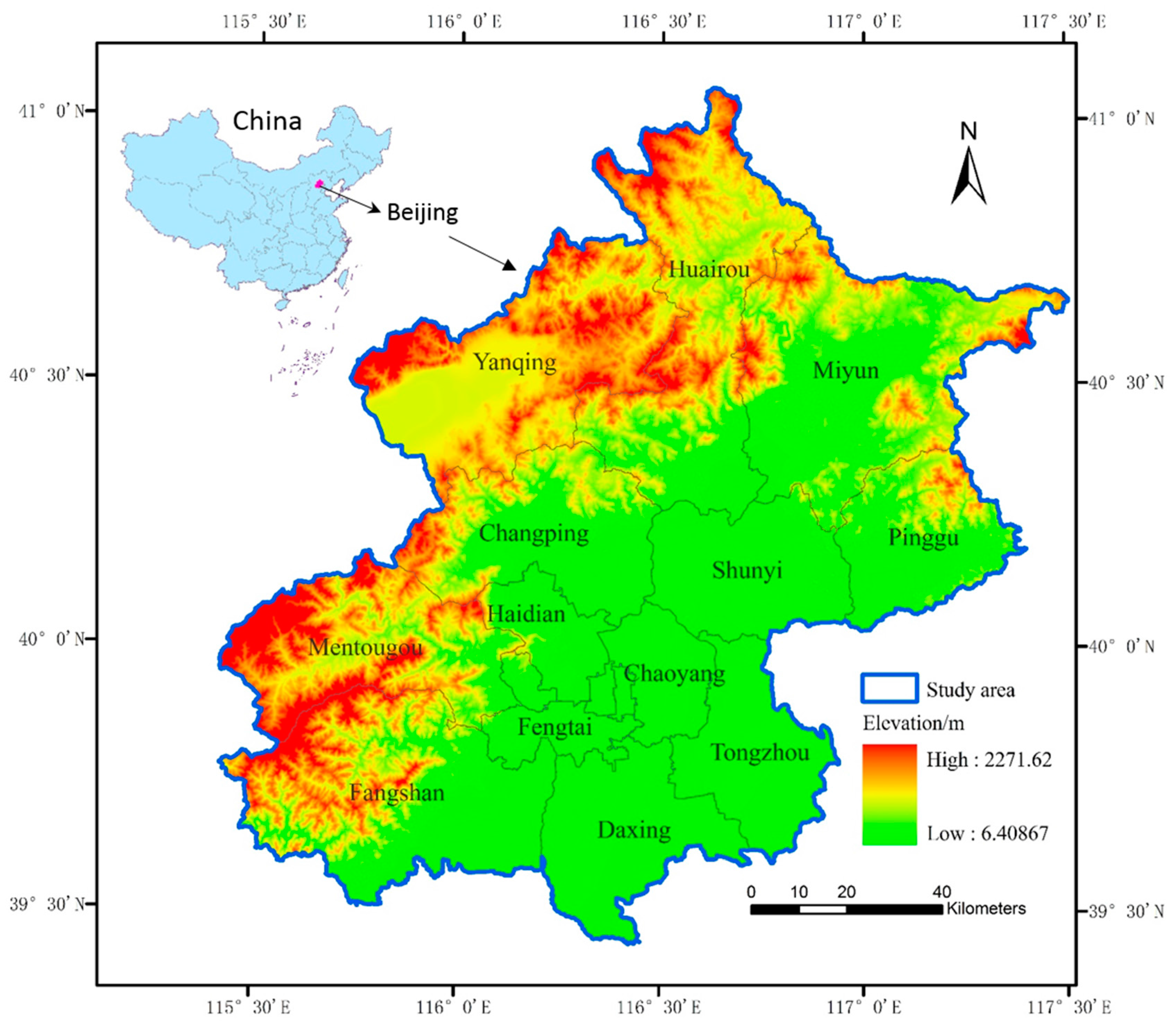
The study area is Beijing, which is located in the northwest of the North China Plain between longitudes 115°25′–117°30′ E and latitudes 39°28′–41°05′ N (Figure 1). The area is 16,411 km2, and there are 16 districts. The city is characterized by alluvial plains in the south and east accounting for 38% of the total area, and hills and mountains in the north, northwest, and west accounting for 62% of the total. The average elevation of Beijing is 43.5 m. The area has a warm, temperate, semi-humid continental monsoon climate with an average annual temperature of 12.5 °C and an average precipitation of 566.1 mm. In 2015, Beijing’s gross domestic product (GDP) topped 2.301 trillion Yuan, and its population was 21.71 million [38].
The primary land use and land cover types in the area can be divided into six general categories: cropland, woodland, grassland, water body, built-up land, and unused land (including sandy land, bare soil, and rock). Woodlands include forests, plantations, shrubs, and others (e.g., orchards). The main tree species [39] in this area are Platycladus orientalis, Pinus tabulaeformis, Larix gmelinii, Quercus spp., Populus davidiana, Robinia pseudoacacia, and Prunus persica.
2.2. Data and Data Processing
The vegetation index products MOD13Q1 Collection 6 contain 12 layers at a 250-m spatial resolution, of which the Normalized Difference Vegetation Index (NDVI) layer is used in this study [40]. The 16-day composites as a gridded level-3 product in the Sinusoidal projection from the National Aeronautics and Space Administration (NASA) MODIS data product website (http://modis.gsfc.nasa.gov) have been derived from the atmospherically-corrected 8-day composite products (MxD09A1) [41]. The study area is covered by two MOD13Q1 scenes (h26v04 and h26v05), and a set of 23 time-phase images covered the full year of 2010. Data processing was supported by ENVI 5.1 (Environment for Visualizing Images). The downloaded MOD13Q1 datasets for the study area were first converted by file formatting, mosaicked, and re-projected into the UTM Zone 50N projection with the WGS 84 datum using nearest neighbor resampling. The NDVI time series datasets were smoothed using a Savitzky-Golay filter [42]. A seven-point quadratic smooth was adopted in this study and convolution weights for quadratic smoothing and differentiation were shown in [43]. A spatial subset was extracted based on the Beijing boundary with a size of 776 rows and 770 columns.
The China Land Use and Land Cover Data Set (CLUCDS) for 2010 was provided by the Data Center for Resources and Environmental Sciences, Chinese Academy of Sciences (RESDC) [22,44]. The dataset included six classes (provincial and national cropland, woodland, grassland, water body, built-up land, and unused land) and 25 subclasses of land use and land cover based on visual interpretation and digitalization with technical support from Intergraph MGE (Modular GIS Environment) software of the Landsat Thematic Mapper (TM) and HJ-1 data at a 30-m spatial resolution [45]. The accuracy of the six classes of land use/cover was above 94.3%, and the overall accuracy of the 25 subclasses was above 91.2% in 2010 [22]. This level of accuracy is acceptable for this study.
2.3. Methods
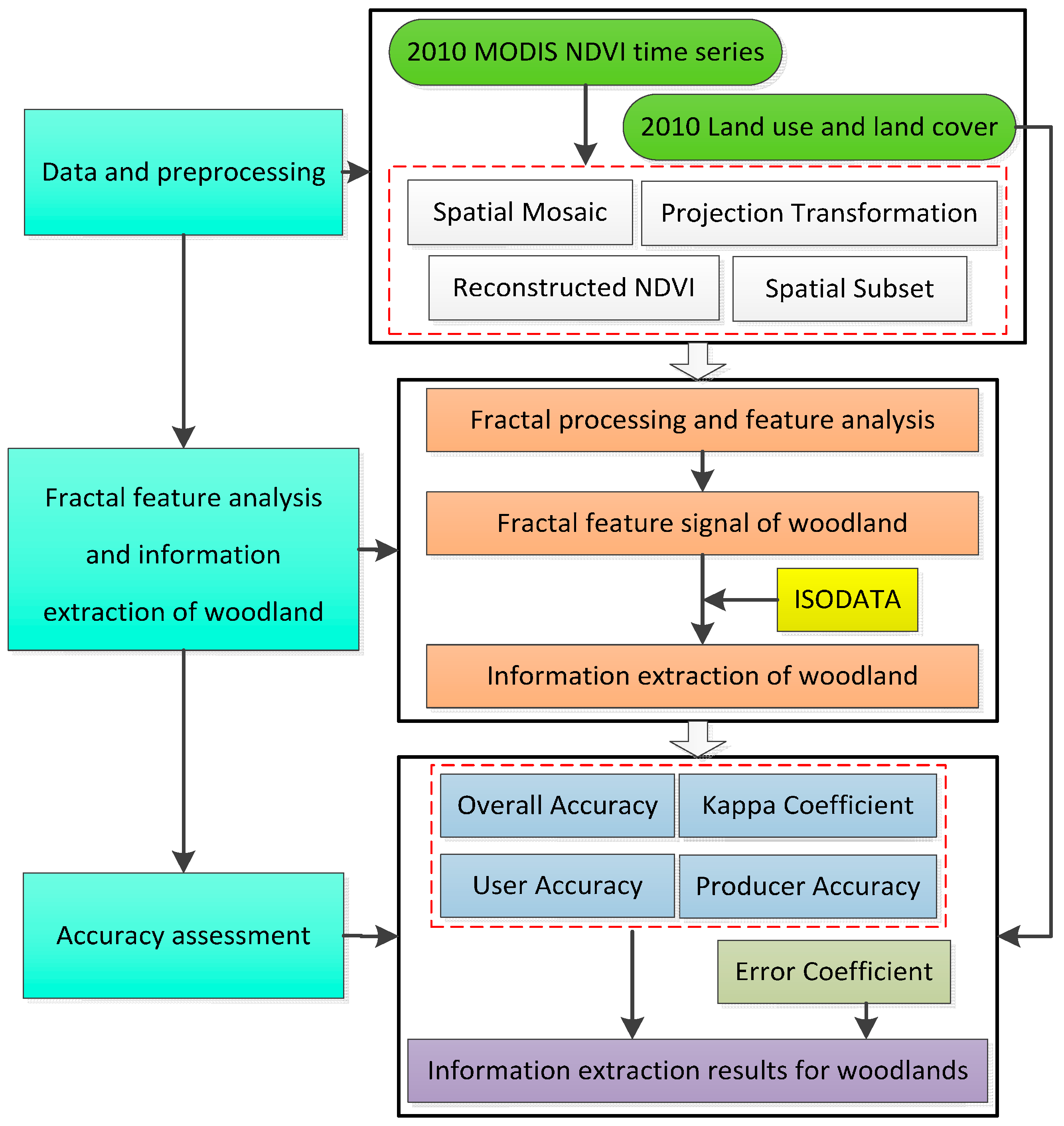
The information extraction method for woodlands in this study has three main parts, including data and preprocessing, fractal feature analysis, and woodland information extraction and extraction accuracy assessment. A flowchart of the information extraction process for woodlands is given in Figure 2. The blanket method and Iterative Self-Organizing Data Analysis technique (ISODATA) tool were adopted for fractal processing of the NDVI time series and the extraction of information on woodlands, respectively. A confusion matrix and error coefficient were employed to assess the accuracy of the extracted results. Fractal computer programs were developed using IDL (Interactive Data Language). The ISODATA analysis and accuracy assessment were performed in the ENVI 5.1 and ArcGIS 9.3 software.
Comparative experiments on the fractal-based and NDVI-based groups were set up to analyze the main contributions of fractal feature. The methods for the information extraction and accuracy assessment in both groups were the same.
2.3.1. Blanket Method
The blanket method was proposed by Peleg et al. [26] to compute the spatial fractal dimension of remote sensing images. Fractal analysis is beneficial in pattern recognition, texture analysis, and image classification. The essence of the method is that a curve (e.g., a spectral curve or time series curve) is developed using different mathematical transformations to select suitable characteristic values for different targets from the perspective of statistics or signal analysis. The principle of this method is that a remote sensing image is treated as a 3-D topography, and the gray of each pixel equates to the height. The terrain surface is then enveloped by two blankets, one on each side, with a distance of ε, and the fractal dimension of the image can be computed by the relationship between the area of the blankets and the volume of the space enveloped by the two blankets. Currently, fractals are mainly used to calculate the spatial fractal dimension of each band in image space, and the process is repeated. This calculation is time-consuming. A fractal dimension calculating the time series curve for each pixel was adopted in this study. The specific method and formula are shown in [26,46]. Both methods were adopted and modified to compute the fractal dimension of the MODIS NDVI time series curves in this study.
A MODIS NDVI time series curve g(i) (i = 1, 2, 3, …, m, where m is the number of samples in NDVI time series), can be enveloped by two curves with a width of 2ε (ε = 1, 2, 3, …, n), where ε is a defined measured unit. The enveloping curves are called upper profiles uε (i) and lower profiles bε (i).
where j is an immediate neighbor of i.
The area of the region enveloped by the upper and lower profiles is calculated using:
The length of the curve is defined as:
According to Mandelbrot’s definition, the length of the fractal curve can be expressed as:
where F is a constant, ε is the measured unit, and D is a parameter related to fractal dimension. For each ε (ε = 2, 3, 4, …, n), three points (log(ε − 1), log(A(ε − 1))), (log(ε), log(A(ε))), (log(ε + 1), log(A(ε + 1))) are adopted to fit a line, and the slope of the fitted line is defined as the fractal signal S(ε) corresponding to the ε.
The complex shape of the real curve results in an asymmetrical length measured under different scales. The curve is measured from the upper side and lower side; thus, Equation (3) becomes:
Correspondingly, the upper length A+(ε) and lower length A−(ε) are defined as:
The fractal signals obtained from Equations (8) and (9) are the upper fractal signal and lower fractal signal, respectively.
2.3.2. Accuracy Assessment
In this study, the China Land Use and Land Cover Data Set (CLUCDS) for Beijing in 2010 was adopted as the reference data and the results of woodlands based on fractal extraction were selected to evaluate. The two classes in this evaluation were woodland and non-woodland. The total samples of CLUCDS were used for accuracy assessment based on the Confusion Matrix tool and this process was performed in the ENVI 5.1 and ArcGIS 9.3 software. The accuracy indices [47] selected to assess the extracted results were overall accuracy (OA), producer accuracy (PA), user accuracy (UA), kappa coefficient (Kappa), and error coefficient (Error). These indices are defined as follows:
where N is the total number of pixels; i is the class (woodland and non-woodland); pii refers to the number of pixels that were correctly classified; pi+ is the number of pixels in the extracted results based on the MODIS NDVI time series; p+i stands for the number of pixels in the CLUCDS for Beijing; Si+ is the total area of the extracted results for woodlands; S+i stands for the area of woodlands in the CLUCDS. The evaluation data and reference data have much better consistency when the value of the calculated error coefficient is smaller.
3. Results
3.1. Fractal Features and Analysis
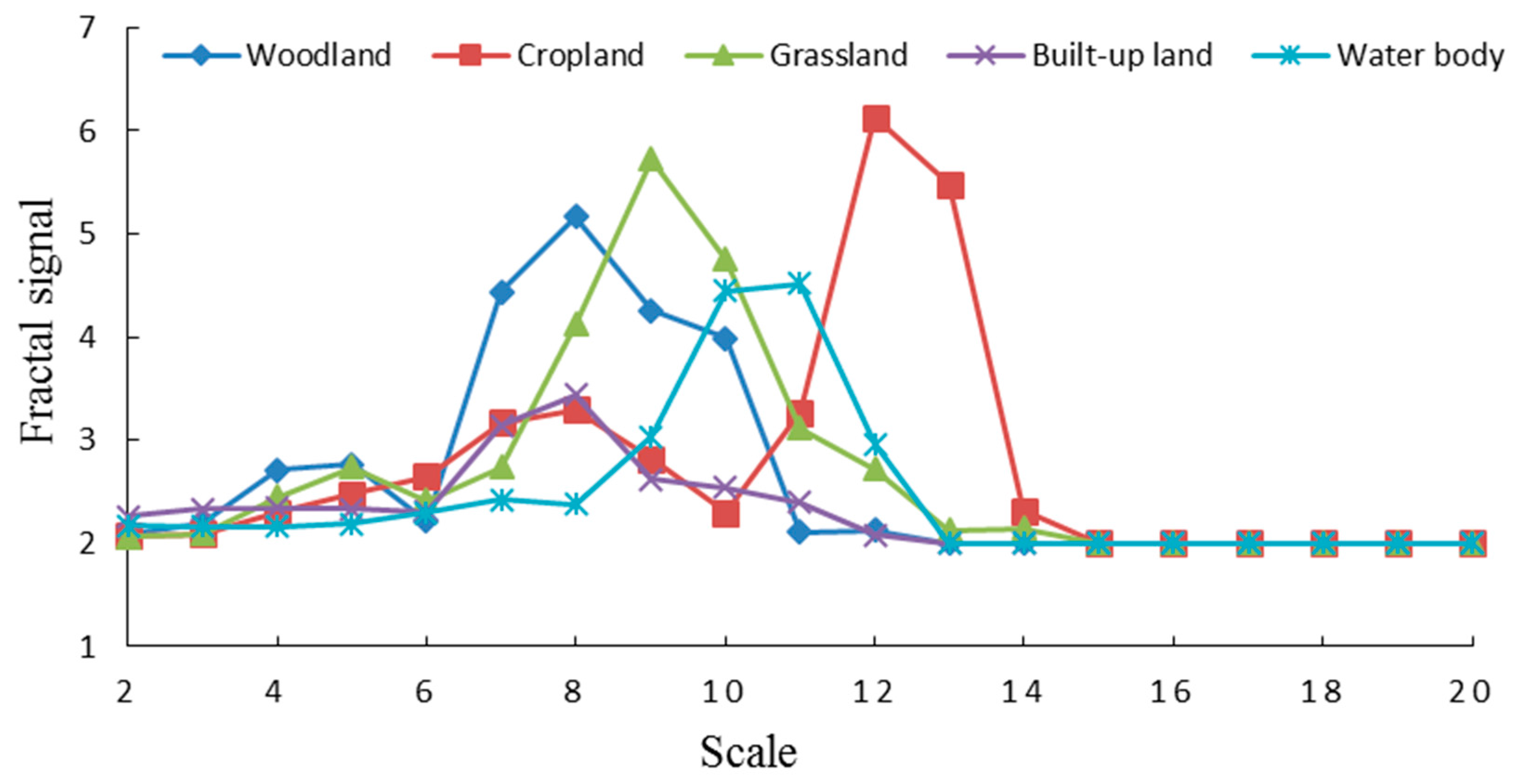
Fractal profile and signal images were obtained after fractal processing. The pixel signal value in each fractal image reflects the complexity of the variation in the NDVI time series curve for a certain measurement unit. The fractal signal value was much higher when the shape of the NDVI time series curve had a more complex variation. The scale with the highest signal value and the most obvious distinction from the other targets in a fractal image was defined as the fractal feature scale of the target.
Five typical targets were selected for reference to their NDVI time series curves and CLUCDS in order to analyze the fractal features of different targets: woodland, cropland, grassland, built-up land, and water body. Six pixels were randomly selected for each target, and their average was taken as the fractal profile of the given target. Figure 3 and Figure 4 are the upper and lower fractal profiles of the different targets with measure units ε (ε = 2, 3, 4,…, 20), respectively. In the figures, the x-axis “scale” n denotes the nth iteration based on Equations (1) and (2).
The fractal features of the different targets were analyzed based on the fractal profile and signal images, and the results were as follows:
- (1)
- The upper and lower fractal profiles and signal images were different. The upper fractal signals of different targets were mainly concentrated at measure units ε 6 to 14 and the lower fractal signals were mainly located at ε 2 to 8.
- (2)
- Both the upper and lower fractal signal values of different targets were different at the same measure unit, and the fractal signal value of the same object had a clear distinction at the different measure units.
- (3)
- Four typical targets, woodland, cropland, grassland, and water body, could be clearly identified at the upper fractal profiles and signal images. Woodland and grassland were also different from other classes at lower fractal profiles and signal images. The fractal profiles and signal images of built-up land had no obvious variation at the upper and lower fractal. The fractal results were decided by the shape or complexity of the NDVI time series curves for the given target.
- (4)
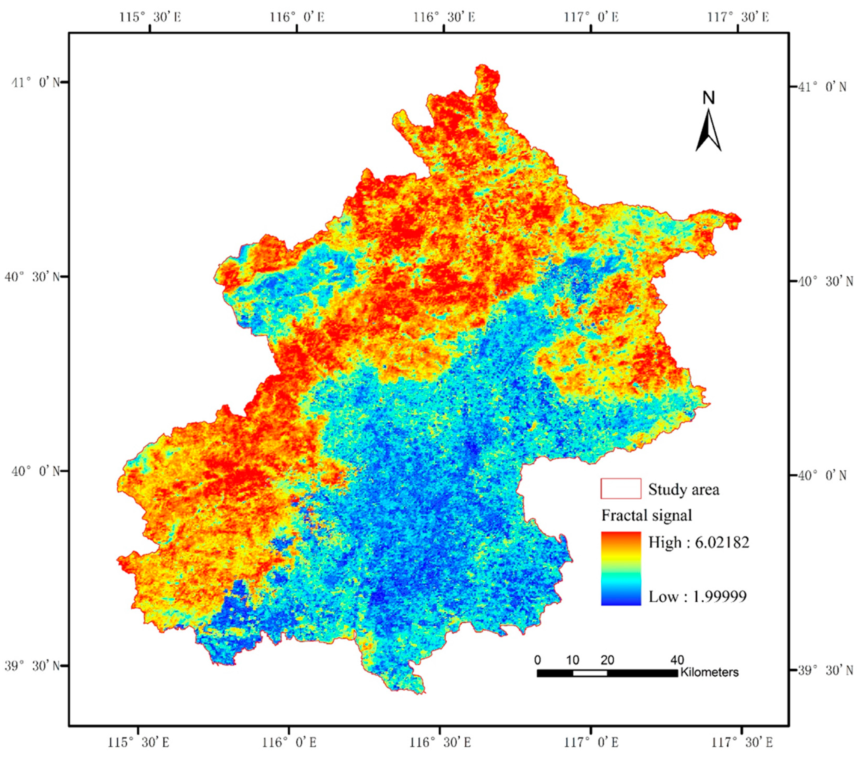
- Woodland was reflected at upper fractal profiles of ε = 8 and lower fractal profiles of ε = 5. The size of the fractal signal value and its difference from other targets were taken into account to choose the fifth scale of the lower fractal as the defining fractal feature scale of woodland. Figure 5 is the lower fractal signal image of ε = 5. The image is expressed with color to increase the visual contrast and separability, and woodland is displayed in red in the image.
- (5)
- The results show that fractals can reveal clear separations of different targets at different scales, and a higher precision of information extraction or classification may be expected based on fractal features.
3.2. Information Extraction and Accuracy Assessment
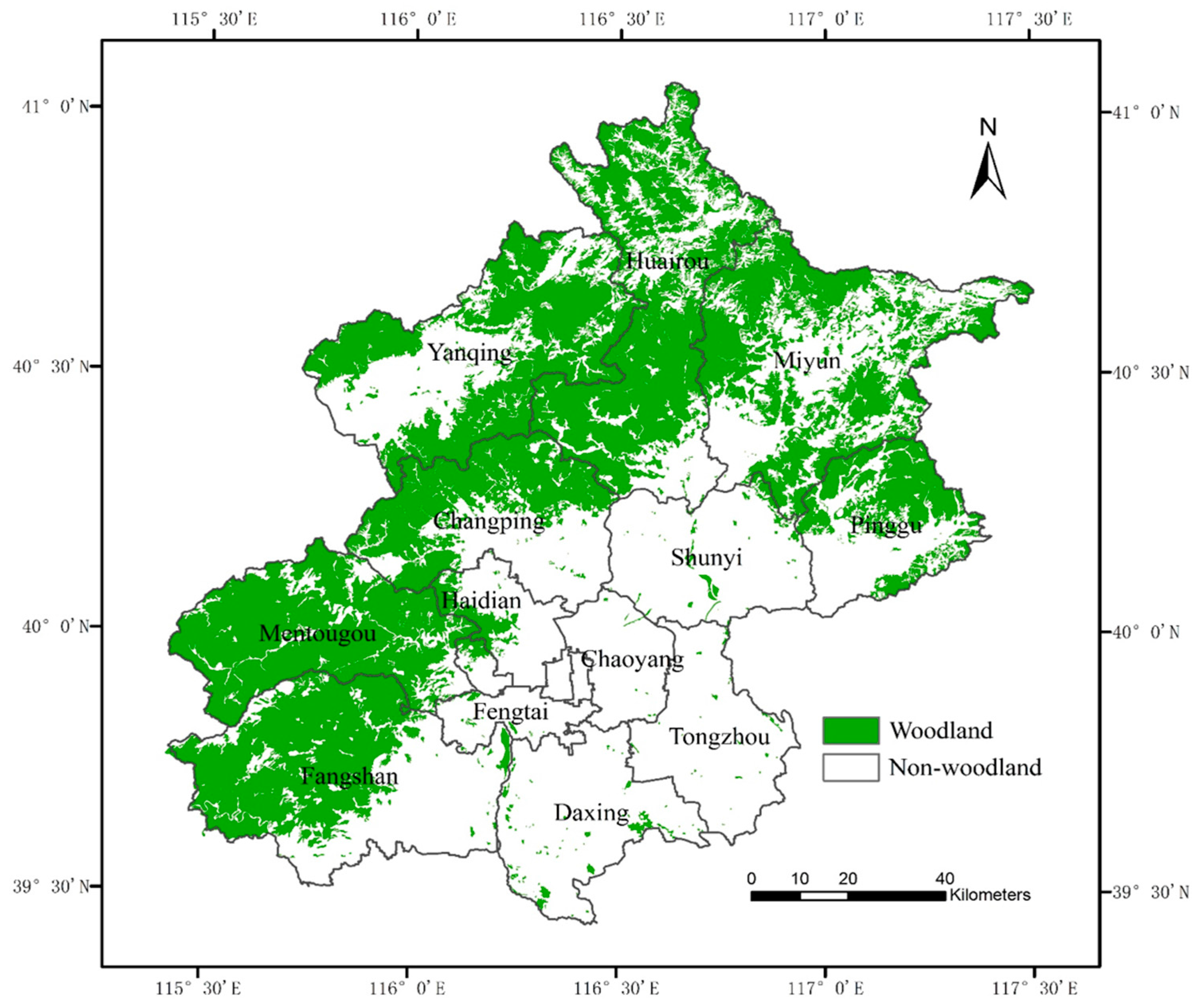
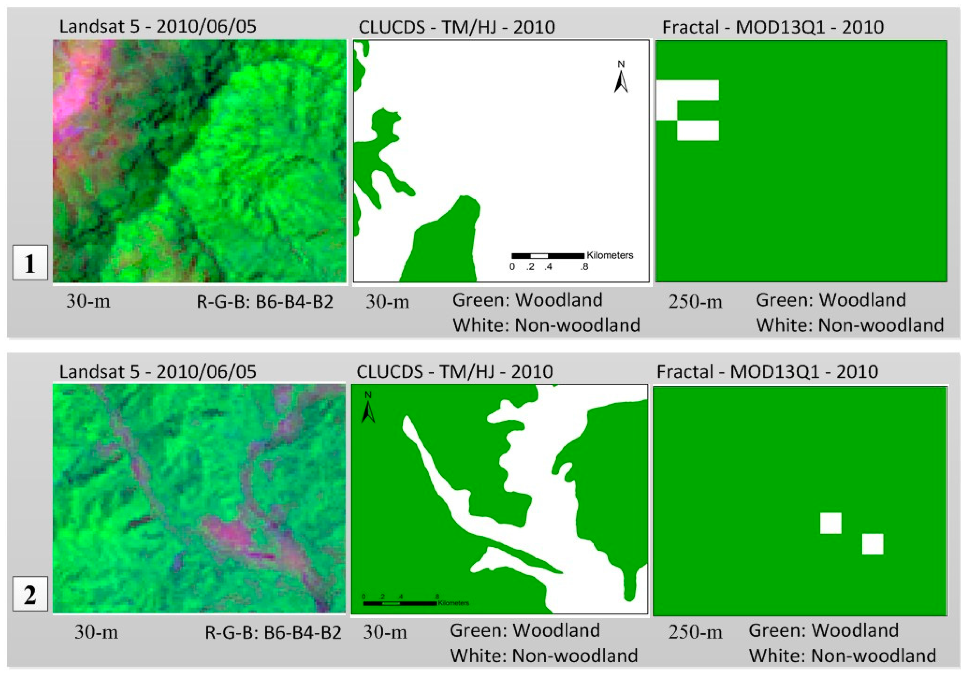
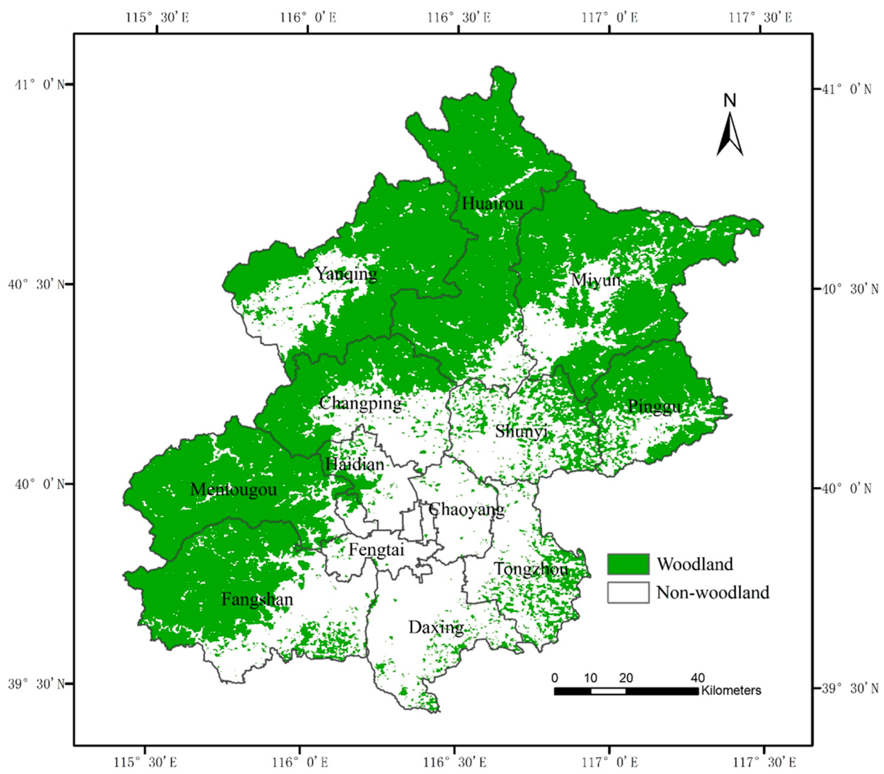
The fifth scale of the lower fractal profile proved to be the fractal feature scale of woodland, and a fractal signal image was selected to extract information for woodlands. The ISODATA tool in ENVI 5.1 was used for this process. The spatial distribution of woodlands is shown in green in Figure 6. The CLUCDS-based spatial distribution of woodlands is shown in Figure 7, also in green. The results of fractal extraction were highlighted by means of subsets, as depicted in Figure 8. Two typical subsets were selected and analyzed. The first subregion (Row 1 in Figure 8), located in the north of Mentougou district, was mainly dominated by woodlands and the results showed that the fractal method in this study could accurately and effectively extract woodland information. The second subregion (Row 2 in Figure 8), located in the west of Huairou district, was covered by woodland and non-woodland and the fractal method could not reveal clear separations of different targets. The spatial distribution of woodlands based on fractal extraction (Figure 6, Row 2 in Figure 8) had a higher density than woodlands in the CLUCDS dataset (Figure 7, Row 2 in Figure 8). This may be due to the spatial resolution of the remote sensing data that were used. The results of Figure 6 and Figure 7 were based on 250-m and 30-m spatial resolution, respectively (Figure 8). Some other fragmented land cover types may have been falsely classified as woodland in the low spatial resolution remote sensing data, as depicted in Figure 8 (Row 2).
An accuracy assessment of the results was conducted using the 2010 CLUCDS dataset. OA, PA, UA, Kappa, and Error were used to quantitatively evaluate the results. The two classes in this evaluation were woodland and non-woodland. The total area was computed as the product of pixel numbers and per pixel area. The total extracted fractal area of woodland was 7984.712 km2, and the total area of woodlands in Beijing from the CLUCDS dataset was 7381.399 km2 in 2010. The accuracy assessment of woodlands based on the fractal extraction is shown in Table 1. Compared with the woodland results in CLUCDS, the OA, Kappa, and Error of the results based on fractal extraction were 90.54%, 0.74, and 8.17%, respectively.
3.3. Comparative Analysis of the Extracted Results and Accuracy Assessment
3.3.1. Comparison with Related Studies
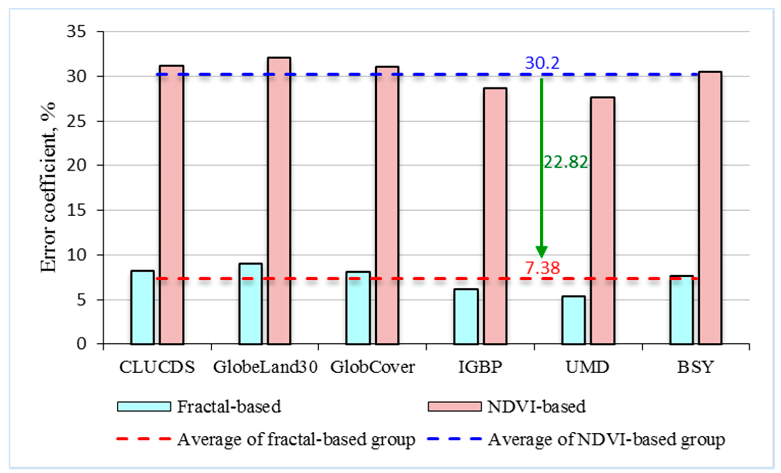
A comparative analysis of this study and related studies was performed. The examined studies included five land cover datasets and one survey statistics dataset. Five land cover datasets were selected, including the China Land Use and Land Cover Data Set (CLUCDS) of the RESDC [22,44]; the GlobeLand30 datasets of the National Geomatics Center of China (NGCC) [25,48]; the GlobCover dataset from the European Space Agency [49]; the MODIS land cover type product MCD12Q1 (International Geosphere Biosphere Programme (IGBP)), and the University of Maryland (UMD) land cover types from NASA [50]. The Beijing Statistical Yearbook (BSY) was chosen for survey statistics data [38]. Only the area and error coefficient (Error) of the extracted results were selected for comparison and analysis because of the limitations of the data formats, data sources, and spatial resolution of the seven datasets chosen. There were two groups, the fractal-based group and the NDVI-based group. The fractal-based group was detailed in this study, whereas woodlands were directly extracted based on using MODIS NDVI time series data only in the NDVI-based group (Section 3.3.2). The results of the comparative analysis are shown in Table 2, and the error coefficients of the fractal-based and NDVI-based groups are shown in Figure 9.
The total extracted area of woodlands in Beijing for the fractal-based group, NDVI-based group, and the related studies in Table 2 were 7984.712 km2, 9682.340 km2, and 7329.068–7583.750 km2, respectively. The error coefficient of the extracted results based on fractal features ranged from 8.95 to 5.29%, and the average was 7.38% (the red dotted line in Figure 9). The error coefficient in the NDVI-based group ranged from 32.11 to 27.67%, and the average was 30.2% (the blue dotted line in Figure 9). Compared with the extracted results for woodlands in the NDVI-based group, the average error coefficient decreased from 30.2 to 7.38% based on the fractal features of the MODIS NDVI time series (difference of 22.82%, Figure 9).
3.3.2. Fractal-Based and NDVI-Based Comparative Experiments
Comparative experiments were set up to evaluate the information extraction method for woodlands based on the fractal feature of the MODIS NDVI time series in this study. In the NDVI-based group, the same method was adopted to extract the spatial distribution of woodlands using the ISODATA tool in ENVI 5.1, and the extracted results are shown in Figure 10. The total extracted area of woodlands was 9682.340 km2. The same method of accuracy assessment was selected to assess the extracted results of the NDVI-based group using the CLUCDS 2010 dataset for Beijing, and the results are shown in Table 3. Compared with the spatial distribution of woodlands in CLUCDS (Figure 7), woodlands were significantly overestimated for the NDVI-based group, especially in Shunyi and Tongzhou districts in Figure 10. This was mainly caused by the method confusing woodland and cropland. In Table 3, the accuracy of the fractal-based group was better than that of the NDVI-based group except for the PA. The fractal features of woodlands in particular contributed to the Error reduction from 31.17 to 8.17%.
4. Discussion
4.1. Theoretical Assumptions
Fractal objects have two basic characteristics [29,51]: (1) infinite detail at every point, and (2) self-similarity between the whole and part of the object. Remote sensing data contain fractal features [37,52]. First, multi-level sequence characteristics obtained at temporal, spatial, or spectral resolutions of remote sensing subjects can be analyzed and interpreted by multiresolution analysis (MRA), which is based on fractal theory. Second, many objects and phenomena in nature show statistical self-similarity, and these are often research targets for remote sensing. When the spatial or temporal scale is changed, the target structure remains the same, and the change reflects enlargement or reduction, with infinite nesting from the whole to the part. Finally, remote sensing images are projections in two-dimensions of a three-dimensional space, and the tonal surface of the two-dimensional image is also a fractal Brownian surface. Thus, the fractal dimension of the image reflects the fractal characteristics of the target ground surface.
Existing research has shown that fractals can reveal obvious separation of different targets at certain scales [46,53,54]. The fractal feature scales of different targets are related to the sample numbers of the initial curve, the shape or complexity of the curve, and difference between the targets in the study area. The influencing factors are positively correlated with the fractal feature, and curves with more samples, complex variation and separability can identify the fractal features of different targets. The blanket method is suitable for the analysis of time series or hyperspectral remote sensing data. The number of samples in time series remote sensing data in per-year intervals are mainly 12 (per month composite, e.g., TM or MODIS), 23 (16-day composite, e.g., TM or MODIS), 46 (8-day composite, e.g., MODIS), and 73 (5-day composite, e.g., Sentinel-2A/B). Hyperspectral remote sensing data have several hundred spectral bands; for example, Earth Observing-1 (EO-1) Hyperion data have 242 bands. The impact of a curve’s shape or complexity is embodied in the fractal calculation process. The maximum operation (upper curve) tends toward a gradually narrowing trough and smoothing peak, while the inverse is true for the minimum operation (lower curve). The ability to show targets by their fractal feature depends on the shape of their curve or the shape characteristics of the troughs and peaks. Information extraction or classification is easier to implement when there are clear differences between land use and land cover types and classes, for example, vegetation and water or single-cropping and double cropping cropland.
4.2. Applicability of Fractal Method and Significance of Fractal Parameters
The achieved accuracies of the extracted results based on fractal features for Beijing are promising. The comparative analysis results also show that the method developed in this study can accurately and effectively extract woodland information. Good applicability of this method is confirmed by the regional characteristics of woodlands for Beijing and the processes and factors influencing the method developed in this study. The study area has a warm, temperate, semi-humid continental monsoon climate, and the woodland vegetation is mainly deciduous. Deciduous trees cycles can be divided into growing and dormant seasons, and their NDVI time series curves have unique characteristics. Deciduous trees have more complex NDVI time series curves than evergreen trees, and the convergence speed of the fractal calculation for deciduous trees is faster.
The use of phenological information as classification input features has been proven to improve land cover classification [55,56]. Wohlfart et al. [57] presented a classification procedure using spectral, phenology-based metrics and ancillary information, particularly for regions comprising complex and heterogeneous environmental conditions. This study demonstrates that fractal parameters are also effective for classification and the method based on the fractal features has broad potential in LUCC detection and the evaluation of major forestry and ecological projects, especially for the rapid identification of woodland expansion and potential damage from natural disasters. Fractals are key indicators that are significant for related research on woodlands, especially for the identification of woodland change. The mutation of fractal features arises mainly from the morphological changes of the woodland NDVI time series curve using the same remote sensing data source and a single target. The combinations of morphological and phenological characteristics and the time nodes of the curve were used to identify abnormal areas and nodes of woodland. It is important to accurately know the location and time of woodland events, which may include afforestation, planting, fire, deforestation, diseases, and insect attacks. Specific research and analysis should be developed to determine event attributes, and this should be combined with auxiliary knowledge and information.
4.3. Support for Government Projects Using the Information Extraction Method for Woodlands
The Chinese/Beijing government launched many ecological restoration projects to alleviate environmental degradation, for example, the Grain for Green Project, the Beijing–Tianjin Sandstorm Source Controlling Project, and the Beijing Plain Afforestation Project. Evidence from remote sensing and statistics data showed that vegetation cover has largely improved, and forest coverage increased [11,38]. Major conservation policies have improved environmental and ecological conditions in this region. Land cover modification was frequently caused by human activities, so we presented a rapid and effective information extraction method to support woodland management and sustainable use. The method developed in this study can be used for feature analysis, information extraction, pattern recognition, and image classification. It is both a low-cost and high-precision method, especially for low spatial resolution remote sensing data and large-scale studies. This method is being applied to extract woodland information for spatial and temporal analysis to evaluate the effectiveness and sustainability of Chinese/Beijing government projects. Thus, this method may have potential in LUCC detection and the evaluation of major ecological forestry projects in China.
5. Conclusions
This paper proposed a low-cost and high-precision information extraction method for woodlands based on fractal features. The results show that fractals can reveal clear separations of different targets at different scales, and the fifth scale of the lower fractal signal was selected as the fractal feature scale for woodlands. The overall accuracy, kappa coefficient, and error coefficient of the extracted results were 90.54%, 0.74, and 8.17%, respectively. Compared with the extracted results for woodlands based only on the MODIS NDVI time series, the average error coefficient decreased from 30.2 to 7.38% based on the fractal features of the MODIS NDVI time series. The results specifically highlighted differences between woodlands and other land use and land cover types.
The method developed in this study is effective for information extraction, pattern recognition, and image classification of woodlands and is being applied to extract data on woodlands for the analysis of spatial and temporal variation to evaluate the effects of Chinese/Beijing government reforestation projects. This method is simple and efficient and has broad potential in LUCC detection and the evaluation of major forestry and ecological projects in China, especially for the rapid identification of woodland expansion and potential damage from natural disasters. This study can enhance understanding of current conditions and provide essential information to support decision-making for woodland management and sustainable use.
Acknowledgments
This study is supported by the Beijing Excellent Talent Support Program (No. 2015000020060G136), the National Key Research and Development Program of China (No. 2016YFD0800904), and the National Natural Science Foundation of China (No. 41071146). We are very grateful to Ziyong Zhou for his helpful suggestions on the fractal computer programs and to NASA, RADI, and RESDC for their data products.
Author Contributions
Shiwei Dong proposed the hypothesis, designed and performed the experiments, and wrote the paper; Hong Li contributed to the experimental design and analyzed the data; Danfeng Sun revised the research design and manuscript.
Conflicts of Interest
The authors declare no conflict of interest.
References
- Sterling, S.M.; Ducharne, A.; Polcher, J. The impact of global land-cover change on the terrestrial water cycle. Nat. Clim. Chang. 2013, 3, 385–390. [Google Scholar] [CrossRef]
- Pitman, A.; Avila, F.; Abramowitz, G.; Wang, Y.; Phipps, S.; de Noblet-Ducoudré, N. Importance of background climate in determining impact of land-cover change on regional climate. Nat. Clim. Chang. 2011, 1, 472–475. [Google Scholar] [CrossRef]
- Pielke, R.A. Land use and climate change. Science 2005, 310, 1625–1626. [Google Scholar] [CrossRef] [PubMed]
- Mooney, H.A.; Duraiappah, A.; Larigauderie, A. Evolution of natural and social science interactions in global change research programs. Proc. Natl. Acad. Sci. USA 2013, 110, 3665–3672. [Google Scholar] [CrossRef] [PubMed]
- Chen, X.; Zhao, H.; Li, P.; Yin, Z. Remote sensing image-based analysis of the relationship between urban heat island and land use/cover changes. Remote Sens. Environ. 2006, 104, 133–146. [Google Scholar] [CrossRef]
- Gimona, A.; Poggio, L.; Brown, I.; Castellazzi, M. Woodland networks in a changing climate: Threats from land use change. Biol. Conserv. 2012, 149, 93–102. [Google Scholar] [CrossRef]
- Feng, Z.; Yang, Y.; Zhang, Y.; Zhang, P.; Li, Y. Grain-for-green policy and its impacts on grain supply in west China. Land Use Policy 2005, 22, 301–312. [Google Scholar] [CrossRef]
- Shan, N.; Shi, Z.; Yang, X.; Gao, J.; Cai, D. Spatiotemporal trends of reference evapotranspiration and its driving factors in the Beijing–Tianjin sand source control project region, China. Agric. For. Meteorol. 2015, 200, 322–333. [Google Scholar] [CrossRef]
- Wu, Z.; Wu, J.; Liu, J.; He, B.; Lei, T.; Wang, Q. Increasing terrestrial vegetation activity of ecological restoration program in the Beijing–Tianjin sand source region of China. Ecol. Eng. 2013, 52, 37–50. [Google Scholar] [CrossRef]
- Cao, S.; Li, Y.; Lu, C. A measure of the net value of ecosystem services and the evaluation of Beijing plain afforestation project. Chin. Sci. Bull. 2016, 61, 2724–2729. [Google Scholar]
- Liu, J.; Li, S.; Ouyang, Z.; Tam, C.; Chen, X. Ecological and socioeconomic effects of China’s policies for ecosystem services. Proc. Natl. Acad. Sci. USA 2008, 105, 9477–9482. [Google Scholar] [CrossRef] [PubMed]
- Peng, S.; Piao, S.; Zeng, Z.; Ciais, P.; Zhou, L.; Li, L.; Myneni, R.; Yin, Y.; Zeng, H. Afforestation in China cools local land surface temperature. Proc. Natl. Acad. Sci. USA 2014, 111, 2915–2919. [Google Scholar] [CrossRef] [PubMed]
- Ouyang, Z.; Zheng, H.; Xiao, Y.; Polasky, S.; Liu, J.; Xu, W.; Wang, Q.; Zhang, L.; Xiao, Y.; Rao, E.; et al. Improvements in ecosystem services from investments in natural capital. Science 2016, 352, 1455–1459. [Google Scholar] [CrossRef] [PubMed]
- Yang, J.; Weisberg, P.; Bristow, N. Landsat remote sensing approaches for monitoring long-term tree cover dynamics in semi-arid woodlands: Comparison of vegetation indices and spectral mixture analysis. Remote Sens. Environ. 2012, 119, 62–71. [Google Scholar] [CrossRef]
- Hou, Z.; Xu, Q.; Nuutinen, T.; Tokola, T. Extraction of remote sensing-based forest management units in tropical forests. Remote Sens. Environ. 2013, 130, 1–10. [Google Scholar] [CrossRef]
- Garrity, S.R.; Allen, C.D.; Brumby, S.P.; Gangodagamage, C.; McDowell, N.G.; Cai, D.M. Quantifying tree mortality in a mixed species woodland using multitemporal high spatial resolution satellite imagery. Remote Sens. Environ. 2013, 129, 54–65. [Google Scholar] [CrossRef]
- Xia, J.; Du, P.; He, X.; Chanussot, J. Hyperspectral remote sensing image classification based on rotation forest. IEEE Geosci. Remote Sens. Lett. 2014, 11, 239–243. [Google Scholar] [CrossRef]
- Engler, R.; Waser, L.T.; Zimmermann, N.E.; Schaub, M.; Berdos, S.; Ginzler, C.; Psomas, A. Combining ensemble modeling and remote sensing for mapping individual tree species at high spatial resolution. For. Ecol. Manag. 2013, 310, 64–73. [Google Scholar] [CrossRef]
- Du, L.; Zhou, T.; Zou, Z.; Zhao, X.; Huang, K.; Wu, H. Mapping forest biomass using remote sensing and national forest inventory in China. Forests 2014, 5, 1267–1283. [Google Scholar] [CrossRef]
- Pouliot, D.; Latifovic, R.; Fernandes, R.; Olthof, I. Evaluation of annual forest disturbance monitoring using a static decision tree approach and 250 m MODIS data. Remote Sens. Environ. 2009, 113, 1749–1759. [Google Scholar] [CrossRef]
- Stellmes, M.; Röder, A.; Udelhoven, T.; Hill, J. Mapping syndromes of land change in Spain with remote sensing time series, demographic and climatic data. Land Use Policy 2013, 30, 685–702. [Google Scholar] [CrossRef]
- Liu, J.; Kuang, W.; Zhang, Z.; Xu, X.; Qin, Y.; Ning, J.; Zhou, W.; Zhang, S.; Li, R.; Yan, C.; et al. Spatiotemporal characteristics, patterns, and causes of land-use changes in China since the late 1980s. J. Geogr. Sci. 2014, 24, 195–210. [Google Scholar] [CrossRef]
- Xu, L.; Li, B.; Yuan, Y.; Gao, X.; Zhang, T.; Sun, Q. Detecting different types of directional land cover changes using MODIS NDVI time series dataset. Remote Sens. 2016, 8, 495. [Google Scholar] [CrossRef]
- Kurnar, D. Monitoring forest cover changes using remote sensing and GIS: A global prospective. Res. J. Environ. Sci. 2011, 5, 105–123. [Google Scholar]
- Chen, J.; Chen, J.; Liao, A.; Cao, X.; Chen, L.; Chen, X.; He, C.; Han, G.; Peng, S.; Lu, M.; et al. Global land cover mapping at 30 m resolution: A pok-based operational approach. ISPRS J. Photogramm. Remote Sens. 2015, 103, 7–27. [Google Scholar] [CrossRef]
- Peleg, S.; Naor, J.; Hartley, R.; Avnir, D. Multiple resolution texture analysis and classification. IEEE Trans. Pattern Anal. Mach. Intell. 1984, 6, 518–523. [Google Scholar] [CrossRef] [PubMed]
- Jolliffe, I. Principal Component Analysis; Wiley Online Library: New York, NY, USA, 2002. [Google Scholar]
- Torrence, C.; Compo, G.P. A practical guide to wavelet analysis. Bull. Am. Meteorol. Soc. 1998, 79, 61–78. [Google Scholar] [CrossRef]
- Mandelbrot, B.B.; Aizenman, M. Fractals: Form, chance, and dimension. Phys. Today 1979, 32, 65. [Google Scholar] [CrossRef]
- Xia, Y.; Feng, D.; Zhao, R. Morphology-based multifractal estimation for texture segmentation. IEEE Trans. Image Process. 2006, 15, 614–623. [Google Scholar] [PubMed]
- Guo, Q.; Shao, J.; Guo, F.; Ruiz, V. Classification of mammographic masses using geometric symmetry and fractal analysis. Int. J. Comput. Assist. Radiol. Surg. 2007, 2, 336–338. [Google Scholar]
- Bishop, M.P.; Shroder, J.F., Jr.; Hickman, B.L.; Copland, L. Scale-dependent analysis of satellite imagery for characterization of glacier surfaces in the Karakoram Himalaya. Geomorphology 1998, 21, 217–232. [Google Scholar] [CrossRef]
- Parrinello, T.; Vaughan, R. Multifractal analysis and feature extraction in satellite imagery. Int. J. Remote Sens. 2002, 23, 1799–1825. [Google Scholar] [CrossRef]
- Weng, Q. Fractal analysis of satellite-detected urban heat island effect. Photogramm. Eng. Remote Sens. 2003, 69, 555–566. [Google Scholar] [CrossRef]
- Myint, S. Fractal approaches in texture analysis and classification of remotely sensed data: Comparisons with spatial autocorrelation techniques and simple descriptive statistics. Int. J. Remote Sens. 2003, 24, 1925–1947. [Google Scholar] [CrossRef]
- Chaudhuri, B.B.; Sarkar, N. Texture segmentation using fractal dimension. IEEE Trans. Pattern Anal. Mach. Intell. 1995, 17, 72–77. [Google Scholar] [CrossRef]
- Sun, W.; Xu, G.; Gong, P.; Liang, S. Fractal analysis of remotely sensed images: A review of methods and applications. Int. J. Remote Sens. 2006, 27, 4963–4990. [Google Scholar] [CrossRef]
- Beijing Municipal Bureau of Statistics; NBS Survey Office in Beijing. Beijing Statistical Yearbook 2016; China Statistics Press: Beijing, China, 2016. [Google Scholar]
- Wang, X.; Niu, S.; Kan, Z. Properties and flammability of major tree species in the Beijing area. Front. For. China 2009, 4, 304–308. [Google Scholar] [CrossRef]
- Didan, K. MOD13Q1 MODIS/Terra Vegetation Indices 16-Day L3 Global 250 m SIN Grid V006; NASA EOSDIS Land Processes DAAC; NASA: College Park, MD, USA, 2015.
- Huete, A.; Didan, K.; Miura, T.; Rodriguez, E.; Gao, X.; Ferreira, L. Overview of the radiometric and biophysical performance of the MODIS vegetation indices. Remote Sens. Environ. 2002, 83, 195–213. [Google Scholar] [CrossRef]
- Chen, J.; Jönsson, P.; Tamura, M.; Gu, Z.; Matsushita, B.; Eklundh, L. A simple method for reconstructing a high-quality NDVI time-series data set based on the Savitzky–Golay filter. Remote Sens. Environ. 2004, 91, 332–344. [Google Scholar] [CrossRef]
- Gorry, P. General least-squares smoothing and differentiation by the convolution (Savitzky-Golay) method. Anal. Chem. 1990, 62, 570–573. [Google Scholar] [CrossRef]
- Liu, J.; Liu, M.; Tian, H.; Zhuang, D.; Zhang, Z.; Zhang, W.; Tang, X.; Deng, X. Spatial and temporal patterns of China’s cropland during 1990–2000: An analysis based on Landsat TM data. Remote Sens. Environ. 2005, 98, 442–456. [Google Scholar] [CrossRef]
- Liu, J.; Liu, M.; Deng, X.; Zhuang, D.; Zhang, Z.; Luo, D. The land use and land cover change database and its relative studies in China. J. Geogr. Sci. 2002, 12, 275–282. [Google Scholar]
- Dong, P. Fractal signatures for multiscale processing of hyperspectral image data. Adv. Space Res. 2008, 41, 1733–1743. [Google Scholar] [CrossRef]
- Liu, C.R.; Frazier, P.; Kumar, L. Comparative assessment of the measures of thematic classification accuracy. Remote Sens. Environ. 2007, 107, 606–616. [Google Scholar] [CrossRef]
- Chen, J.; Ban, Y.; Li, S. Open access to earth land-cover map. Nature 2014, 514, 434. [Google Scholar] [CrossRef]
- Arino, O.; Bicheron, P.; Achard, F.; Latham, J.; Witt, R.; Weber, J.L. GlobCover the most detailed portrait of earth. ESA Bull. Eur. Space Agency 2008, 136, 24–31. [Google Scholar]
- Friedl, M.A.; Sulla-Menashe, D.; Tan, B.; Schneider, A.; Ramankutty, N.; Sibley, A.; Huang, X.M. MODIS collection 5 global land cover: Algorithm refinements and characterization of new datasets. Remote Sens. Environ. 2010, 114, 168–182. [Google Scholar] [CrossRef]
- Pentland, A.P. Fractal-based description of natural scenes. IEEE Trans. Pattern Anal. Mach. Intell. 1984, 6, 661–674. [Google Scholar] [CrossRef] [PubMed]
- Luan, H.; Tian, Q.; Yu, T.; Hu, X.; Huang, Y.; Du, L.; Zhao, L.; Wei, X.; Han, J.; Zhang, Z.; et al. Modeling continuous scaling of NDVI based on fractal theory. Spectrosc. Spectr. Anal. 2013, 33, 1857–1862. [Google Scholar]
- Riccio, D.; Ruello, G. Synthesis of fractal surfaces for remote-sensing applications. IEEE Trans. Geosci. Remote Sens. 2015, 53, 3803–3814. [Google Scholar] [CrossRef]
- Guan, J.; Liu, N.; Huang, Y.; He, Y. Fractal poisson model for target detection within spiky sea clutter. IEEE Geosci. Remote Sens. Lett. 2013, 10, 411–415. [Google Scholar] [CrossRef]
- Dymond, C.; Mladenoff, D.; Radeloff, V. Phenological differences in Tasseled Cap indices improve deciduous forest classification. Remote Sens. Environ. 2002, 80, 460–472. [Google Scholar] [CrossRef]
- Zhong, L.; Hawkins, T.; Biging, G.; Gong, P. A phenology-based approach to map crop types in the San Joaquin Valley, California. Int. J. Remote Sens. 2011, 32, 7777–7804. [Google Scholar] [CrossRef]
- Wohlfart, C.; Liu, G.; Huang, C.; Kuenzer, C. A river basin over the course of time: Multi-temporal analyses of land surface dynamics in the Yellow River Basin (China) based on medium resolution remote sensing data. Remote Sens. 2016, 8, 186. [Google Scholar] [CrossRef]
Figure 1.
Location of the study area.

Figure 2.
Flowchart of information extraction for woodlands. MODIS, Moderate Resolution Imaging Spectroradiometer; NDVI, normalized difference vegetation index; ISODATA, Iterative Self-Organizing Data Analysis technique.
Figure 2.
Flowchart of information extraction for woodlands. MODIS, Moderate Resolution Imaging Spectroradiometer; NDVI, normalized difference vegetation index; ISODATA, Iterative Self-Organizing Data Analysis technique.

Figure 3.
Upper fractal profiles of different targets.

Figure 4.
Lower fractal profiles of different targets.
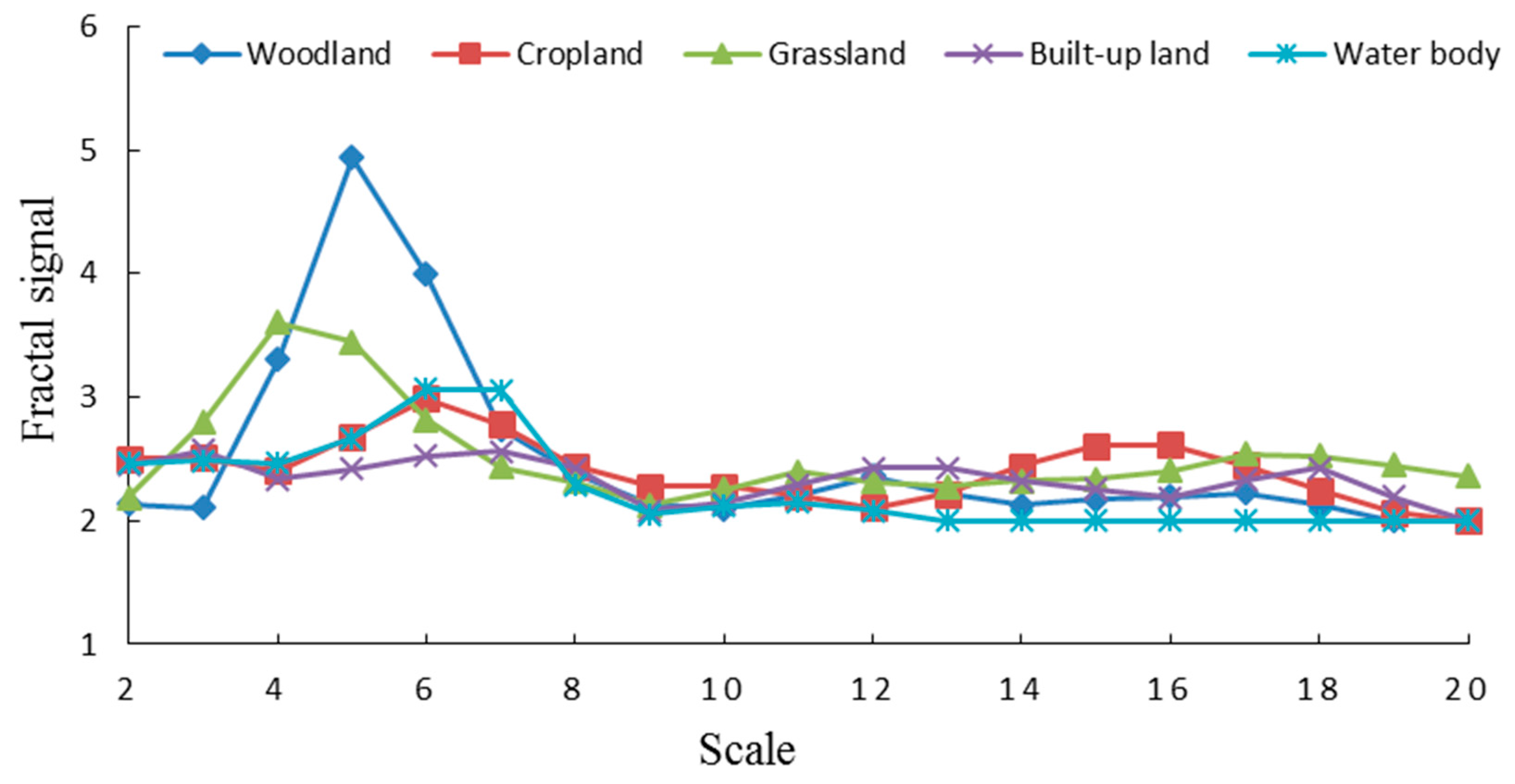
Figure 5.
Lower fractal signal image of ε = 5 (color).

Figure 6.
Spatial distributions of woodlands based on fractal extraction. The subsets were used for detailed exhibition in Figure 8.
Figure 6.
Spatial distributions of woodlands based on fractal extraction. The subsets were used for detailed exhibition in Figure 8.
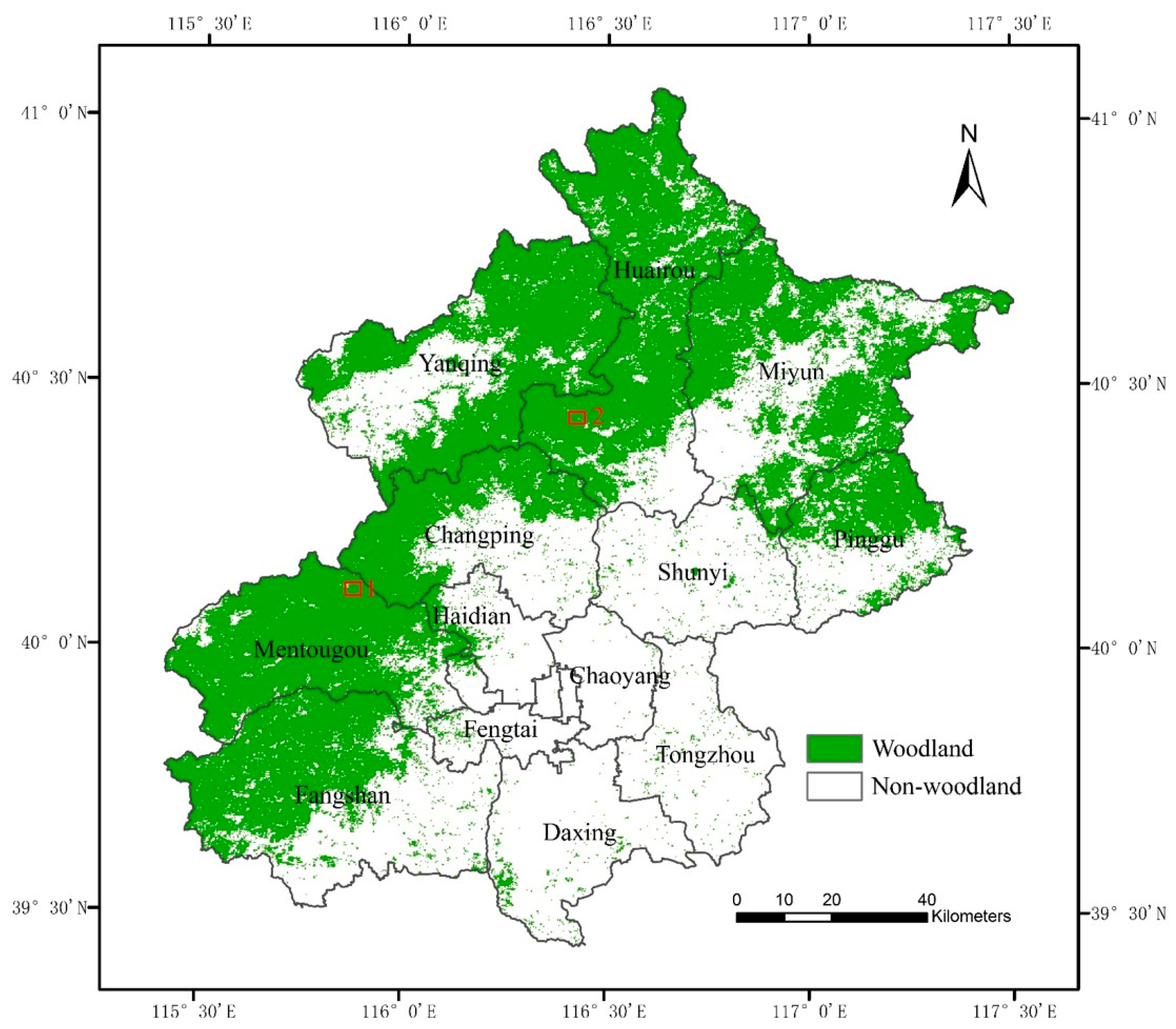
Figure 7.
Spatial distributions of woodlands based on the China Land Use and Land Cover Data Set (CLUCDS).
Figure 7.
Spatial distributions of woodlands based on the China Land Use and Land Cover Data Set (CLUCDS).

Figure 8.
Comparison of Landsat 5 imagery (Column 1), the China Land Use and Land Cover Data Set (CLUCDS; Column 2), and the results of fractal extraction in this study (Column 3). The numbers refer to the exact geographical location as indicated in Figure 6. Landsat 5 imagery (5 June 2010; path/row: 123/032; RGB band combination: 6-4-2) was provided by the Open Spatial Data Sharing Project of Institute of Remote Sensing and Digital Earth (RADI), Chinese Academy of Sciences (http://ids.ceode.ac.cn).

Figure 9.
Error coefficients of fractal-based and NDVI-based groups. IGBP, International Geosphere Biosphere Programme; UMD, University of Maryland; BSY, Beijing Statistical Yearbook.
Figure 9.
Error coefficients of fractal-based and NDVI-based groups. IGBP, International Geosphere Biosphere Programme; UMD, University of Maryland; BSY, Beijing Statistical Yearbook.

Figure 10.
Spatial distributions of woodlands in the NDVI-based group.


Table 1.
Accuracy assessment of woodlands based on fractal extraction compared with the China Land Use and Land Cover Data Set (CLUCDS) for Beijing in 2010.
Table 1.
Accuracy assessment of woodlands based on fractal extraction compared with the China Land Use and Land Cover Data Set (CLUCDS) for Beijing in 2010.
| Indices | PA, % | UA, % | OA, % | Kappa | Error, % |
|---|---|---|---|---|---|
| Woodlands | 83.54 | 77.21 | 90.54 | 0.74 | 8.17 |
PA, producer accuracy; UA, user accuracy; OA, overall accuracy; Kappa, kappa coefficient; Error, error coefficient.
Table 2.
Comparative analysis of this study and related studies in Beijing.
| Datasets | Data Sources | SR | Year | Woodland Area, km2 | Error, % | |
|---|---|---|---|---|---|---|
| Fractal-Based | NDVI-Based | |||||
| MOD13Q1 | MODIS/TERRA | 250 m | 2010 | 7984.712, 9682.340 | / | / |
| CLUCDS | Landsat/TM, HJ/CCD | 30 m | 2010 | 7381.399 | 8.17 | 31.17 |
| GlobeLand30 | Landsat/TM, HJ/CCD | 30 m | 2010 | 7329.068 | 8.95 | 32.11 |
| GlobCover | ENVISAT/MERIS | 300 m | 2009 | 7385.670 | 8.11 | 31.10 |
| MCD12Q1-IGBP | MODIS/TERRA | 500 m | 2010 | 7523.750 | 6.13 | 28.69 |
| MCD12Q1-UMD | MODIS/TERRA | 500 m | 2010 | 7583.750 | 5.29 | 27.67 |
| Beijing Statistical Yearbook (BSY) | Survey Statistics | / | 2010 | 7420.185 | 7.61 | 30.49 |
SR, Spatial Resolution; Error, error coefficient; MOD13Q1, adopted in this study; Fractal-based, 7984.712 km2; NDVI-based, 9682.340 km2; CLUCDS, China Land Use and Land Cover Data Set; “/” means no data.
Table 3.
Comparative analysis of the extracted results and accuracy assessment of the fractal-based and NDVI-based groups compared with the China Land Use and Land Cover Data Set (CLUCDS).
Table 3.
Comparative analysis of the extracted results and accuracy assessment of the fractal-based and NDVI-based groups compared with the China Land Use and Land Cover Data Set (CLUCDS).
| Woodlands | Area, km2 | PA, % | UA, % | OA, % | Kappa | Error, % |
|---|---|---|---|---|---|---|
| Fractal-based | 7984.712 | 83.54 | 77.21 | 90.54 | 0.74 | 8.17 |
| NDVI-based | 9682.340 | 92.73 | 70.68 | 89.48 | 0.73 | 31.17 |
PA, producer accuracy; UA, user accuracy; OA, overall accuracy; Kappa, kappa coefficient; Error, error coefficient.
© 2017 by the authors. Licensee MDPI, Basel, Switzerland. This article is an open access article distributed under the terms and conditions of the Creative Commons Attribution (CC BY) license (http://creativecommons.org/licenses/by/4.0/).
Share and Cite
MDPI and ACS Style
Dong, S.; Li, H.; Sun, D. Fractal Feature Analysis and Information Extraction of Woodlands Based on MODIS NDVI Time Series. Sustainability 2017, 9, 1215. https://doi.org/10.3390/su9071215
AMA Style
Dong S, Li H, Sun D. Fractal Feature Analysis and Information Extraction of Woodlands Based on MODIS NDVI Time Series. Sustainability. 2017; 9(7):1215. https://doi.org/10.3390/su9071215
Chicago/Turabian StyleDong, Shiwei, Hong Li, and Danfeng Sun. 2017. "Fractal Feature Analysis and Information Extraction of Woodlands Based on MODIS NDVI Time Series" Sustainability 9, no. 7: 1215. https://doi.org/10.3390/su9071215
Note that from the first issue of 2016, this journal uses article numbers instead of page numbers. See further details here.