Article

A Performance Evaluation of Dynamical Downscaling of Precipitation over Northern California

1
Water Resources Research Center, K-Water Institute, Daejeon 34045, Korea
2
Department of Civil and Environmental Engineering, University of California, Davis, CA 95616, USA
3
Department of Civil and Environmental Engineering, Kumamoto University, Kumamoto 860-8555, Japan
4
Department of Civil and Architectural Engineering, University of Wyoming, Laramie, WY 82071, USA
5
Department of Environmental Engineering, Toyama Prefectural University, Toyama 939-0398, Japan
6
California Department of Water Resources, Sacramento, CA 95814, USA
7
California Department of Water Resources, Sacramento, CA 95821, USA
8
US Bureau of Reclamation, Sacramento, CA 95825, USA
*
Author to whom correspondence should be addressed.
Sustainability 2017, 9(8), 1457; https://doi.org/10.3390/su9081457
Submission received: 29 June 2017 / Revised: 28 July 2017 / Accepted: 9 August 2017 / Published: 17 August 2017
(This article belongs to the Special Issue Geospatial Technologies for Sustainable Natural Resources)

Abstract

:
It is important to assess the reliability of high-resolution climate variables used as input to hydrologic models. High-resolution climate data is often obtained through the downscaling of Global Climate Models and/or historical reanalysis, depending on the application. In this study, the performance of dynamically downscaled precipitation from the National Centers for Environmental Prediction (NCEP) and the National Center for Atmospheric Research (NCAR) reanalysis data (NCEP/NCAR reanalysis I) was evaluated at point scale, watershed scale, and regional scale against corresponding in situ rain gauges and gridded observations, with a focus on Northern California. Also, the spatial characteristics of the simulated precipitation and wind fields, with respect to various grid sizes, were investigated in order to gain insight to the topographic effect on the atmospheric state variables. To this end, dynamical downscaling was performed using the mesoscale atmospheric model MM5, and the synoptic scale reanalysis data were downscaled to a 3 km grid spacing with hourly temporal resolution. The results of comparisons at point scale and watershed scale over a 50-year time period showed that the MM5-simulated precipitation generally produced the timing and magnitude of the observed precipitation in Northern California. The spatial distributions of MM5-simulated precipitation matched the corresponding observed precipitation reasonably well. Furthermore, the statistical goodness of fit tests of the MM5-simulated precipitation against the corresponding observed precipitation showed the reliability and capability of MM5 simulations for downscaling precipitation. A comparison of the spatial characteristics of the results with respect to various grid sizes indicated that precipitation and wind fields are significantly affected by the local topography. In particular, the banded structures and orographic effects on precipitation and wind fields can be well described by a mesoscale model at 3 km and 9 km grid resolutions while 27 km and 81 km grid model simulation may not be sufficient for watershed-scale or sub-watershed-scale studies.

1. Introduction

GCMs (global climate models) are the primary tools for assessing the magnitude and impacts of climate change on water resources, floods, water quality, sea level rise, ecosystems, etc. Global historical reanalysis datasets such as the National Centers for Environmental Prediction (NCEP) and the National Center for Atmospheric Research (NCAR) reanalysis I [1] data can be used for the reconstruction of historical atmospheric data which can then be utilized as input for hydrologic or environmental modeling of the historical conditions in sparsely gauged or ungauged watersheds [2,3]. However, GCM and reanalysis datasets whose horizontal resolutions are more than 50 km in general are not suitable for the watershed scale because they cannot capture the mesoscale processes such as convection, orographic effects and sharp frontal gradients in order to account for the effect of local land conditions on the climate at these scales [4,5,6,7,8]. The fine spatial and temporal scales are also essential to the modeling of surface and subsurface hydrological processes (e.g., [9,10,11]) due to the heterogeneity in land characteristics within a watershed.
As such, downscaling of the coarse-resolution global datasets becomes necessary to resolve the scale discrepancy between coarse-resolution GCMs (or reanalysis data) and the resolution required for an assessment at a regional scale or a watershed scale. Statistical downscaling and dynamical downscaling approaches are commonly used to resolve the scale discrepancy, but statistical downscaling is not suitable because it fundamentally assumes unchanged statistical relationships and unchanged spatial variability [8,12,13]. Meanwhile, dynamical downscaling by means of a regional climate model (RCM) is a technique that has several valuable features. RCMs are able to represent realistic regional climate features such as orographic precipitation, land surface characteristics [14,15,16], and extreme precipitation (e.g., [17,18]). RCMs can also account for the physical interactions of land-atmospheric processes with consideration of the heterogeneity in topography, soil, vegetation, and climate variables over a watershed by solving the full equation suite of mass, energy, and momentum conservation laws in the atmosphere. Moreover, the complete climate variables including precipitation, air temperature, wind speed, relative humidity, solar radiation, etc., can be produced by RCMs based upon the given GCM outputs or reanalysis data at very fine spatial and temporal resolutions.
On the other hand, the major disadvantage of RCMs is the cost of their numerical computations that place restrictions not only on the simulation period, but also the computational grid size. For this reason, most of the RCM-related studies have been restricted to applications on the assessment of model performance (e.g., [19,20,21,22,23,24]), or on future climate change impact assessment with a relatively coarse grid resolution (normally more than 20 km) over specified time slices (e.g., [25,26,27]), with finer resolution over specified time slices (e.g., [28]), or with relatively coarse grid resolution over a long-term period [29,30].
The accuracy of downscaled climate variables depends on the biases inherited from the driving GCM [4,5] as well as the model characteristics, such as the model formulation, grid resolution, numerical scheme and other physical parameterizations [7,31,32]. GCM simulations of the present-day climate are forced by prescribed sea surface temperatures (SST), and are deterministically predictable in short and middle range [33,34]. Therefore, downscaled results from GCM simulations are comparable to observation data only in climatological features, as in the study by [29]. On the other hand, reanalysis data are the assimilated results from the analysis of various data sources (e.g., land surface, ship, rawinsonde, pibal, aircraft, and satellite), and are consistent with the observations [1]. Thus, downscaled results from reanalysis data have the potential to be used for more detailed comparison with observation data. Hence, reanalysis data are more suitable for the evaluation of downscaling performance.
In this study, dynamically downscaled precipitation, which is already commonly used in climate change impact studies at watershed scales, is used to reconstruct historical climate variables at different scales. The dynamically downscaled precipitation is evaluated at point scale, watershed scale and regional scale against corresponding in situ rain gauges and gridded observations, with a focus on Northern California. A description of the study area and observational datasets is provided, the methodology is demonstrated, and dynamically downscaled precipitation is evaluated. Additionally, the spatial characteristics of the simulated precipitation and wind fields, with respect to various grid sizes, are investigated in order to gain insight to the topographic effect on the atmospheric state variables.

2. Study Area and Methodology
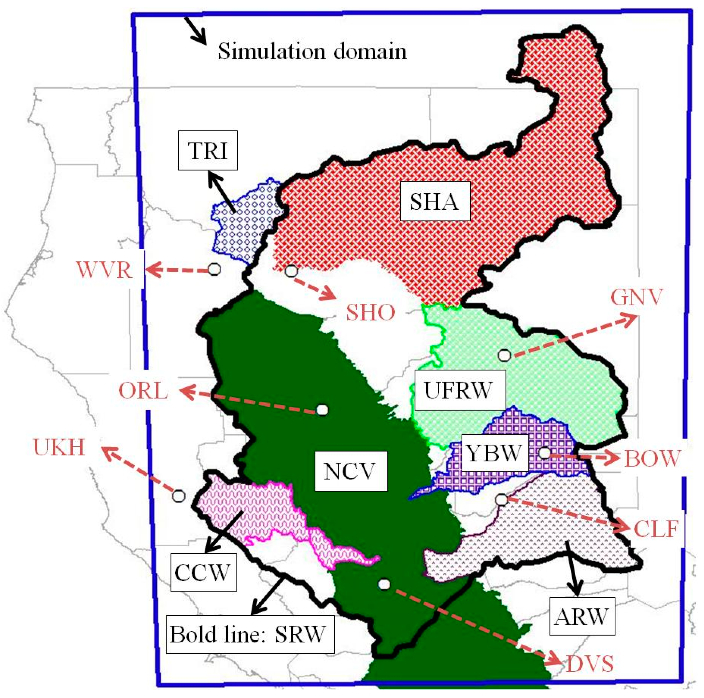
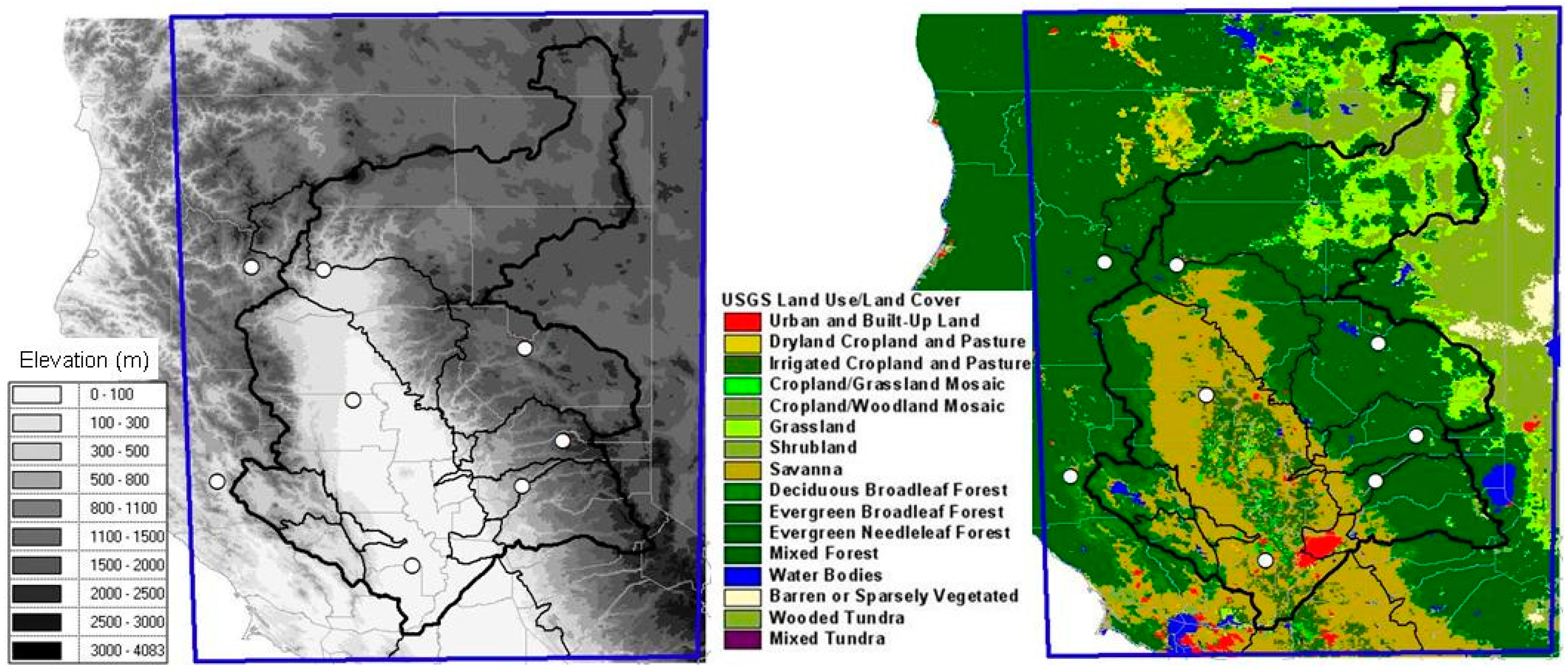
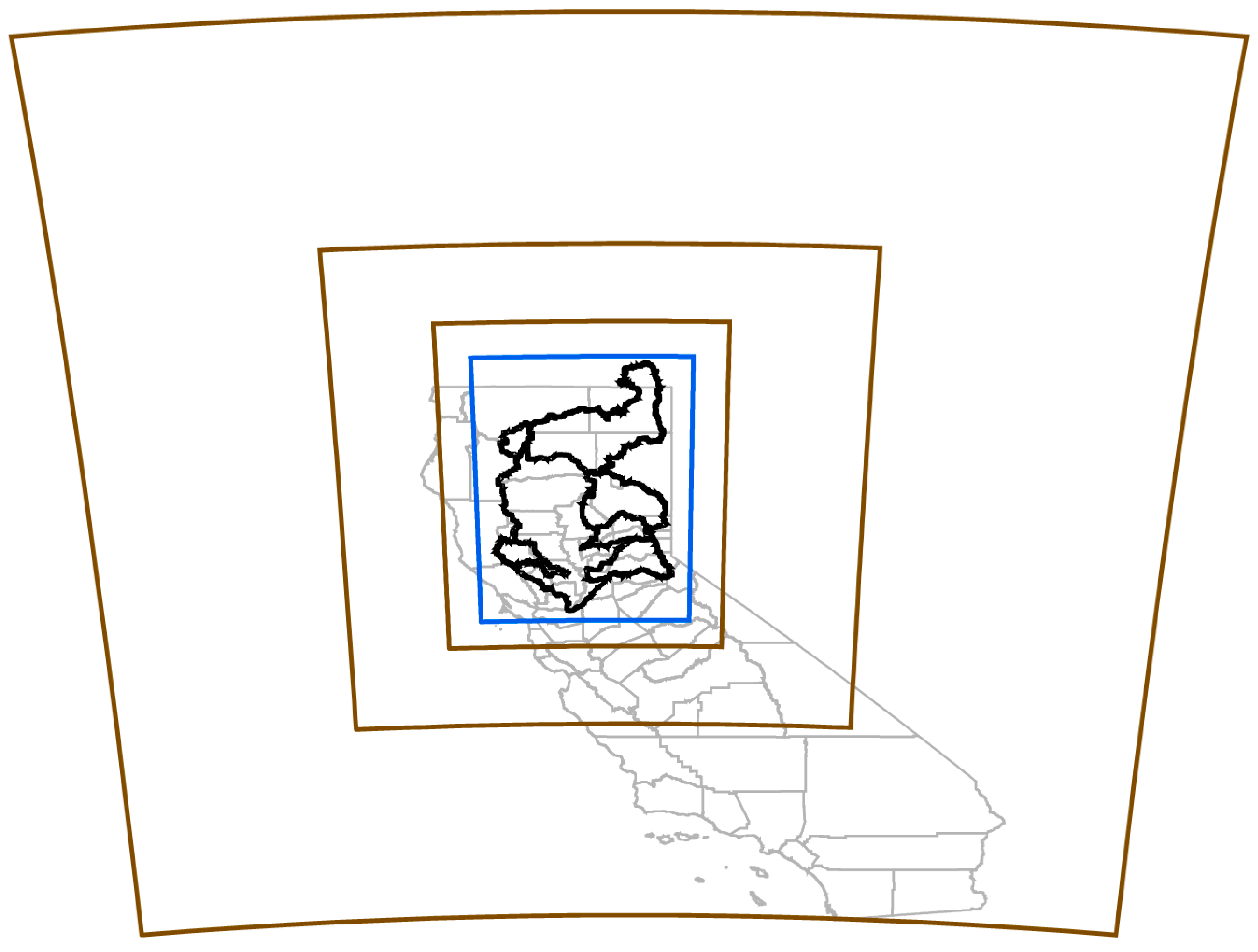
2.1. Study Area

A region of Northern California (see Figure 1) was selected for this study as it is the prime source of water for California. Two-thirds of the precipitation in California falls on the Sacramento River watershed, and 80% of the precipitation occurs between November and March.
Eight watersheds and eight individual ground observation stations were selected for the model performance evaluation considering the location, topography, vegetation, and size of the watershed, as shown in Table 1 and Figure 1. The largest watershed among the study watersheds is the Sacramento River watershed (SRW) which is a fundamental water source, supplying domestic, irrigation, industrial and environmental water in California. It also contributes contaminants and nutrients from agricultural land and mountainous terrain to the Central Valley and Bay-Delta areas. The Central Valley and Bay-Delta areas are crucial regions for agriculture and ecosystems in California. Oroville Dam, Folsom Dam, Shasta Dam, Englebright Dam, and Trinity Dam in the study region control the water resources of Northern California. The Cache Creek watershed (CCW) is a representative hydrologic unit in the Coastal Range, and the Northern Central Valley (NCV) watershed comprises most of the low-lying and agricultural lands in Central California. The Sierra Nevada, Coastal Range, and their foothills recharge the groundwater under the Central Valley, which is a very important source of water during the dry season in California. Elevations, drainage areas and vegetation covers of the selected watersheds are diverse (see Table 1 and Figure 2). For example, mid- and downstream sections of the Upper Feather River watershed (UFRW) and Shasta Dam watershed (SHA) are comprised of forest and steep canyon areas, but upstream sections of these watersheds are flat grasslands and croplands. The northwest coastal region which contains the Trinity dam watershed (TRI), and the Sierra Nevada which contains the American River watershed (ARW), Yuba River watershed (YBW) and downstream of UFRW and SHA in Northern California, receive plenty of precipitation due to a combination of the orographic effect and moisture influx from the Pacific Ocean, which is sometimes referred to as a pineapple express or atmospheric river. For the evaluations at point scale, eight ground stations from the California Data Exchange Center (CDEC, [35]) of the California Department of Water Resources (CDWR) were selected based on their locations and record length (see Figure 1 and Table 1).

2.2. Methodology

In this study, the Fifth-Generation NCAR/Penn State Mesoscale Model, MM5 [38], was set up over the Northern California domain shown in Figure 1, downscaling the NCAR/NCEP reanalysis I data [1,39]) from a 210 × 210 km horizontal grid spacing to a fine-scale 3 × 3 km grid resolution (see Figure 3). Four one-way nested grids are used for this study. Two-way nesting techniques could make the model results more accurate; however, two-way nesting accuracy depends on application regions and it is computationally more expensive and time-consuming than the method applied herein [40].
The simulated precipitation by the MM5 has been successfully validated and used for precipitation analysis over California by several research groups [41,42,43,44]. Furthermore, Ishida et al. [45] showed that the MM5 can occasionally show better precipitation results than a next-generation mesoscale numerical weather prediction system, the Weather Research and Forecasting Model (WRF, [46]), and the MM5 requires less computational costs.
According to the one-third ratio rule of the nesting domain, recommended by [38], the first through fourth nesting domains (D1–D4) were configured with the spatial grid resolutions of 81 km, 27 km, 9 km, and 3 km, respectively. Thus, the domains have 24 × 22, 37 × 31, 73 × 49, and 175 × 109 horizontal grid points, respectively, with 25 vertical levels. MM5 is a nonhydrostatic and fully compressible three-dimensional model which can be downscaled even up to a 1 km spatial resolution. It is hence able to capture the orographic effects and land surface/land use conditions of watersheds.
The NCAR/NCEP reanalysis I data used for the initial and boundary conditions of the MM5 simulations are a combination of a numerical weather model that runs reforecasts over historical periods, assimilating observations from in situ sources such as rawinsonde, marine surface, land surface, aircraft, satellite, and so on [1]. Therefore, the MM5-simulated precipitation from the NCAR/NCEP reanalysis I data may be suitable for evaluating the model performance by comparing it against observations. For the 50-year climate simulation from 1950 to 1999, the model simulation was reinitiated at every water year (from 1 October to 30 September) of the simulation period with an additional two days at the beginning for spin-up. MM5-simulated precipitation over the study area is dominated by boundary conditions. Several trials before the yearly simulations found that initial conditions affect precipitation over the study area only for a few days. In addition, the study area has little precipitation at the beginning of a water year, in early October. Thus, the re-initiation at every water-year during the simulation period does not affect the results of the yearly simulations. No nudging technique was utilized in this study for this reason. On the other hand, all the variables used as boundary conditions, including sea surface temperature, were from the NCAR/NCEP reanalysis data at 6 h temporal resolution.
For the performance evaluation of dynamically downscaled precipitation by MM5, the historical precipitation data were collected from various public sources. This includes eight CDEC ground observation stations from CDWR (see Table 1), PRISM data from the PRISM Climate Group [47], and NCEP/EMC U.S. Gridded Precipitation (gauge-only, radar, and Stage IV) from NCAR/EOL under the sponsorship of the National Science Foundation [48]. The ground-observed precipitation data were used for time-series comparisons at point locations, while PRISM data were used for evaluations of both basin-average precipitation at eight watersheds and for spatial precipitation fields over Northern California. NCEP/EMC U.S. Gridded Precipitation data were used in order to evaluate the spatial variability at hourly, 24 h and monthly time scales within the simulation domain.
It should be noted that model bias correction, which is a common procedure for improving the quality of data reconstruction, has not been used in this study. All evaluation results are based on simulated precipitation without any bias correction in order to test the model performance objectively.

3. Results and Discussion

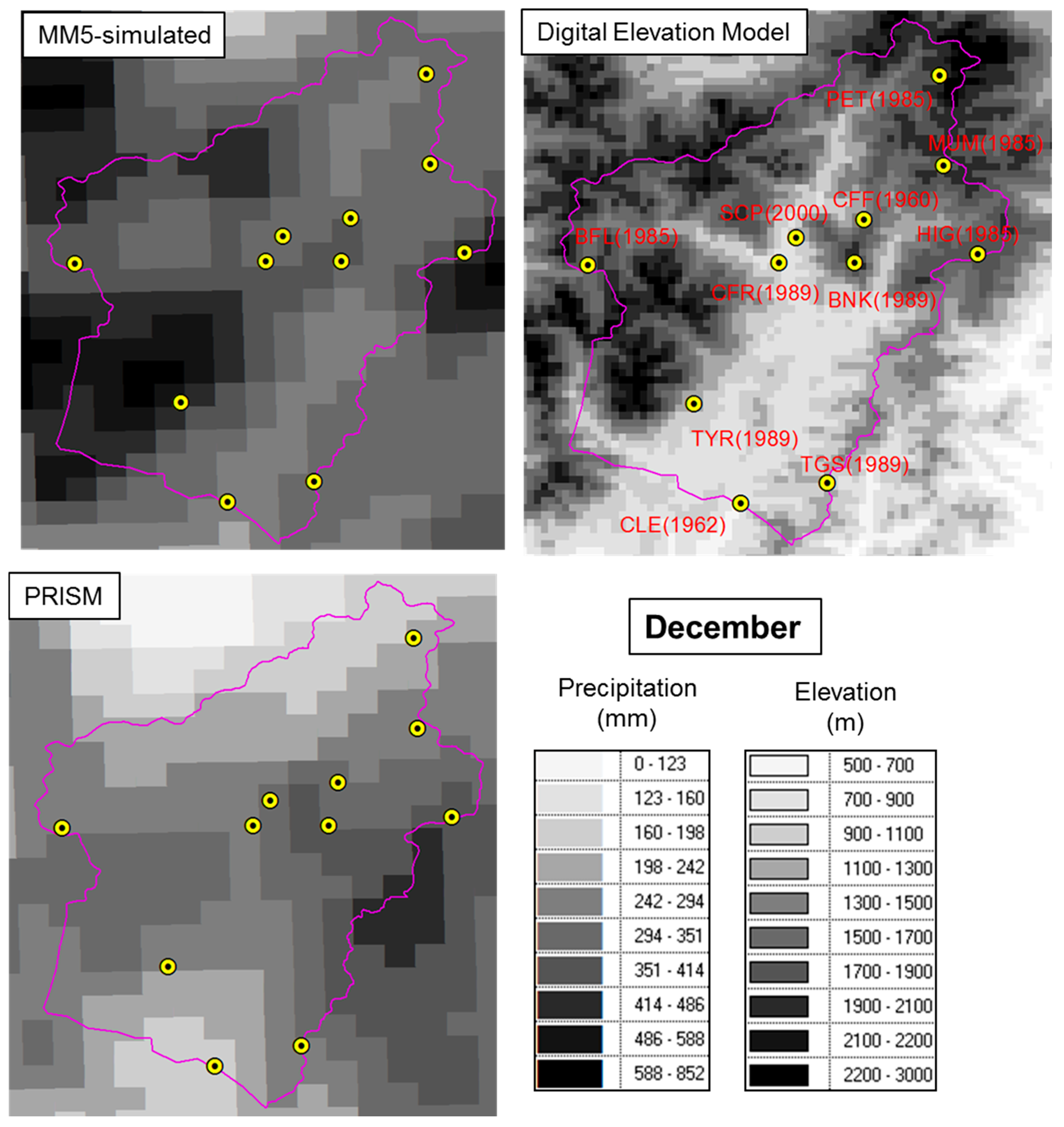
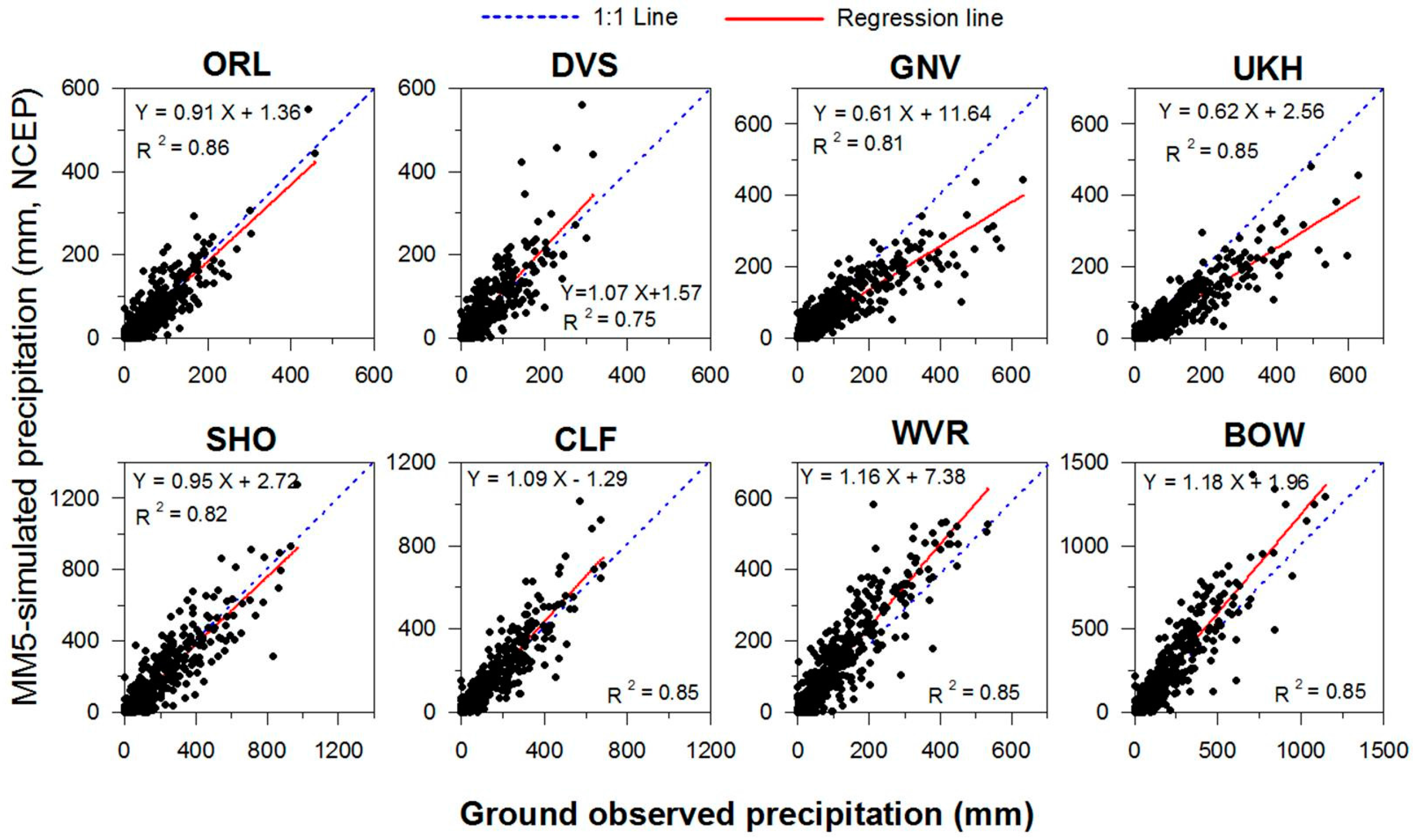
3.1. Evaluation at Point Scale

MM5-simulated precipitation was evaluated by the corresponding ground observations at 8 CDEC stations (see Table 1 and Figure 1). The elevations of the selected eight ground stations range from 18 m to 1641 m.
Scatter graphs of the simulated and observed monthly precipitation at eight ground stations are shown in Figure 4. Although the model slightly underestimates the precipitation at the GNV (Greenville RS) and UKH (Ukiah) stations and overestimates at the WVR (Weaverville RS) and BOW (Bowman) stations, both the observed and the simulated values are generally comparable. The coefficient of determination, R2, values are higher than 0.75. However, the model performance could be different depending on the locations of the gauging stations within the watersheds. Hence, it may not be appropriate to evaluate the downscaling performance by comparisons at only a few gauging station point locations.

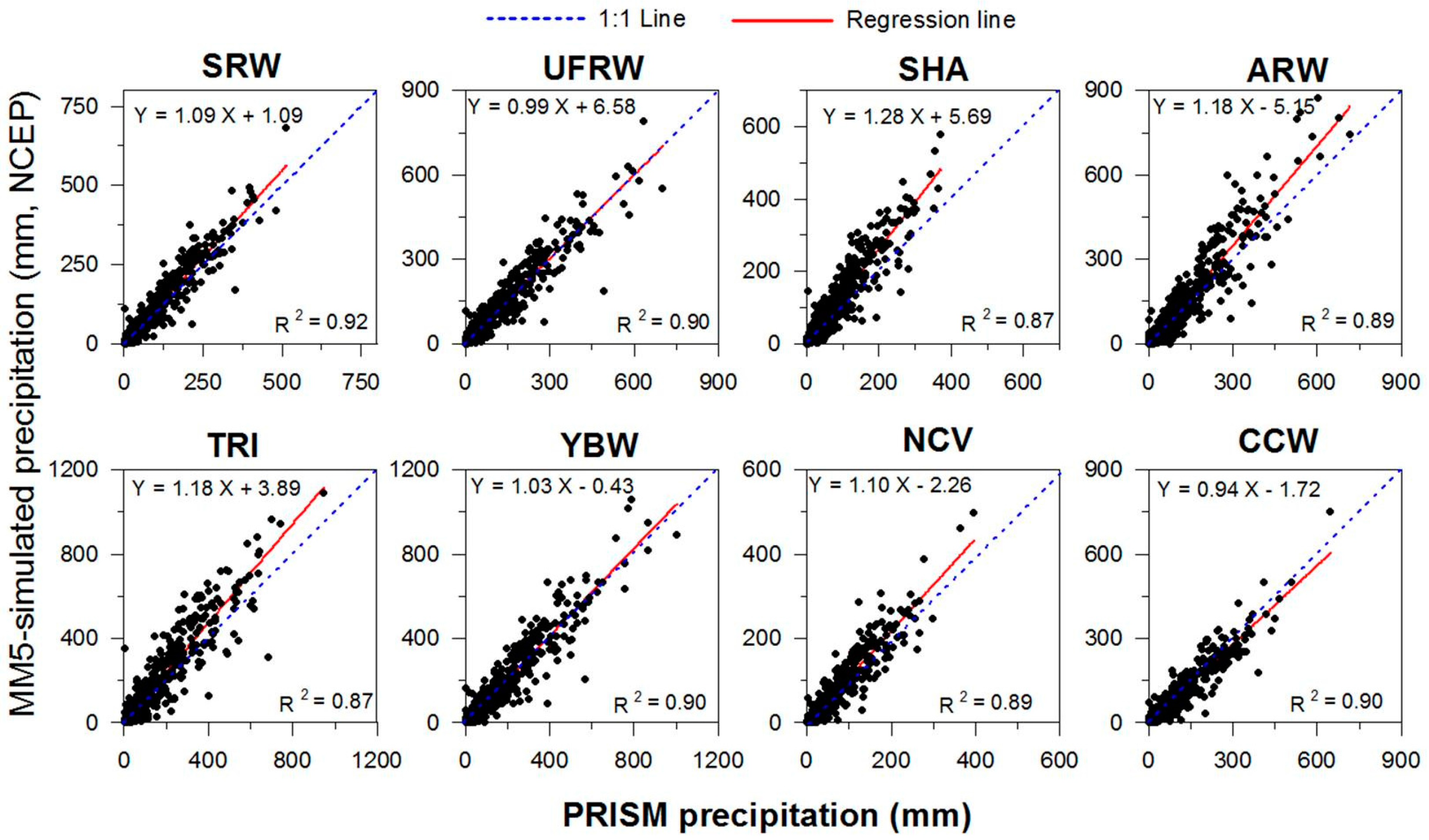
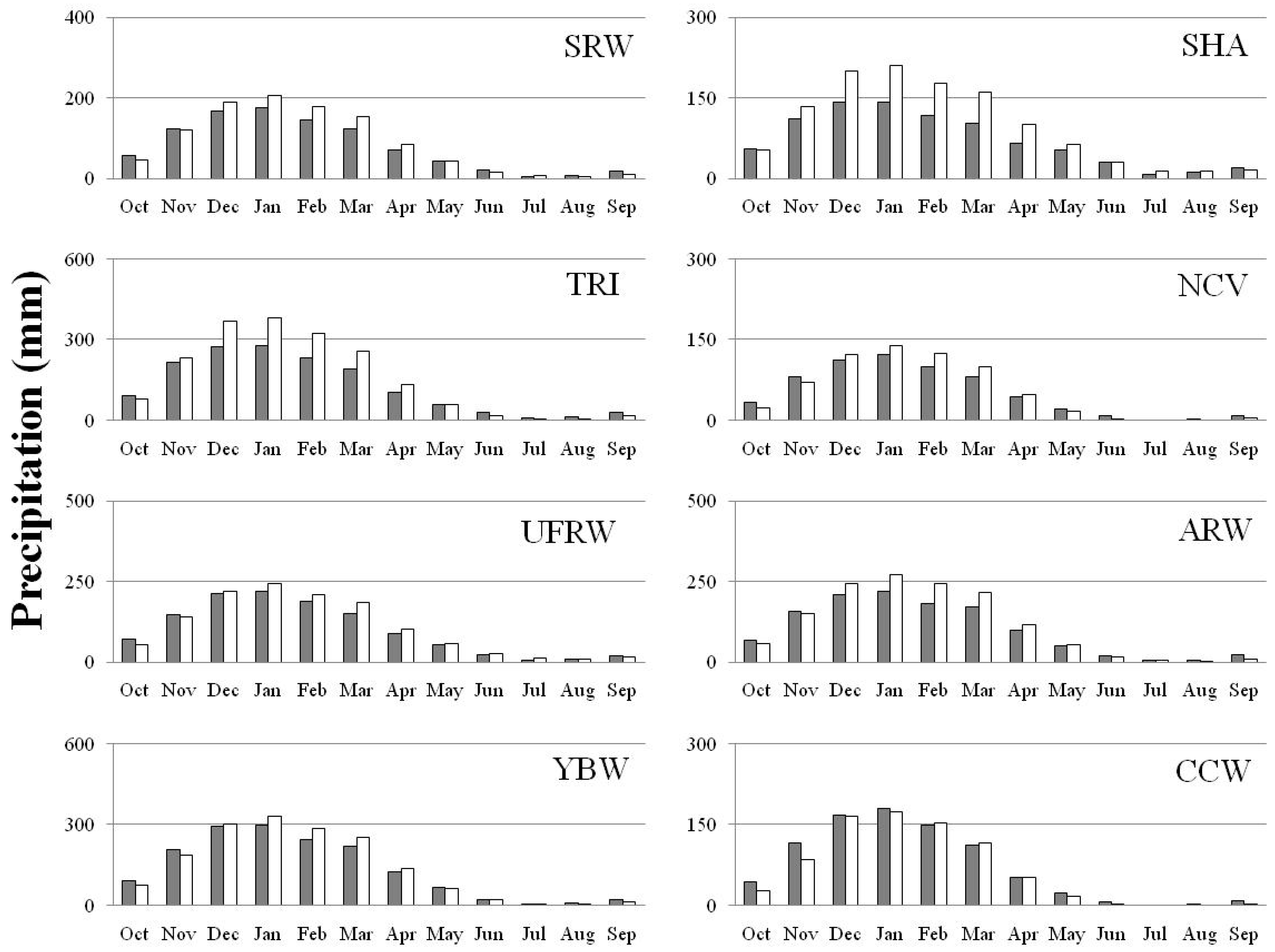
3.2. Evaluation at Watershed Scale

For evaluation at the scale of watersheds, MM5-simuated precipitation values were compared against the corresponding PRISM (parameter-elevation regressions on independent slopes model, [49]) precipitation data at eight watersheds within the simulation domain. PRISM provides interpolated ground precipitation data over the United States at 4 km horizontal grid spacing from 1895 to the present [47].
As stated previously in the section on the study area, the selected eight watersheds have various characteristics with respect to topography, geomorphology, vegetation, drainage area, and climate. Figure 5 shows the scatter plots of basin-average precipitation between PRISM and MM5-simulated precipitation for eight Northern California watersheds during 1950–1999. Among the eight watersheds, the MM5-simulated precipitation for SHA, TRI and ARW is slightly higher than the PRISM precipitation at higher values. These three watersheds are located in high-elevation mountainous terrain. MM5-simulated and PRISM precipitation values were also evaluated by statistical comparisons of the means, standard deviations (STDEV), coefficients of determination (R2), root-mean-square errors, and Nash-Sutcliffe efficiency (ENS) during 1950 to 1999 for the eight watersheds (Table 2). The means and STDEVs are similar to the PRISM values. High values of R2 and ENS were found at the eight watersheds.

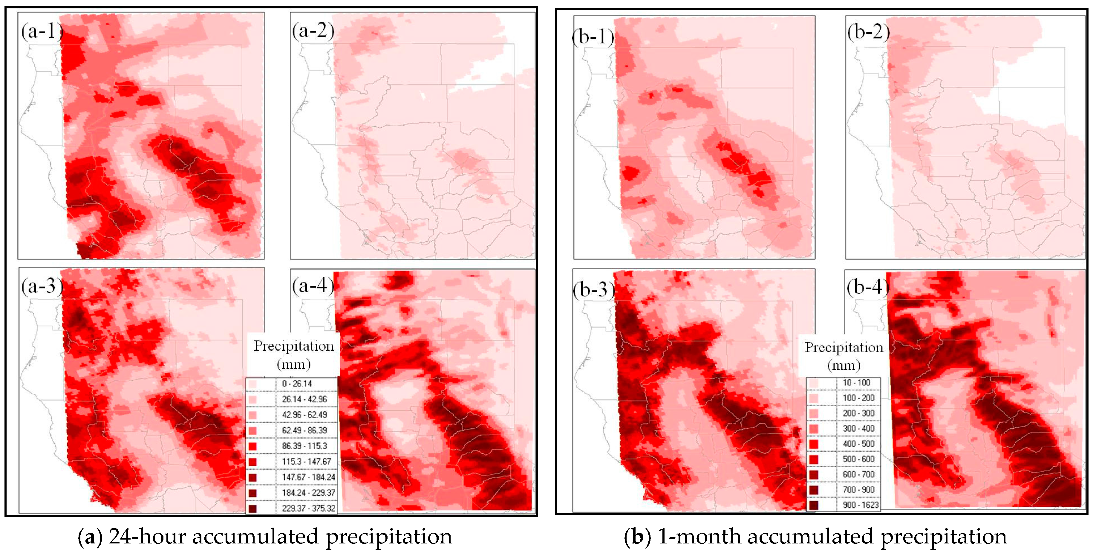
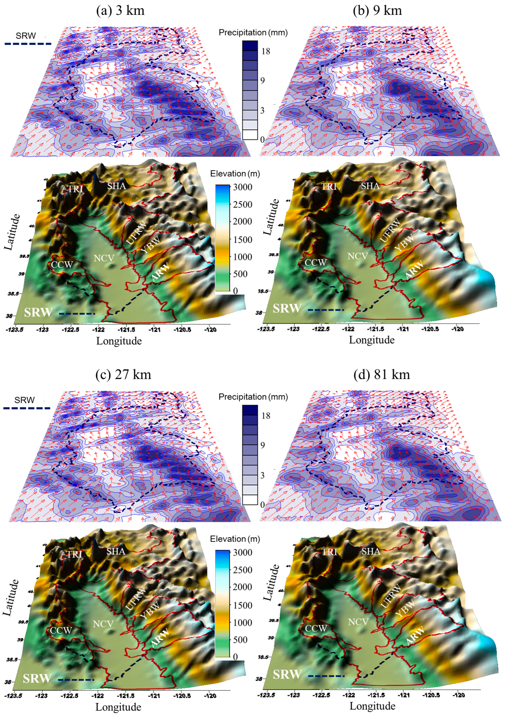
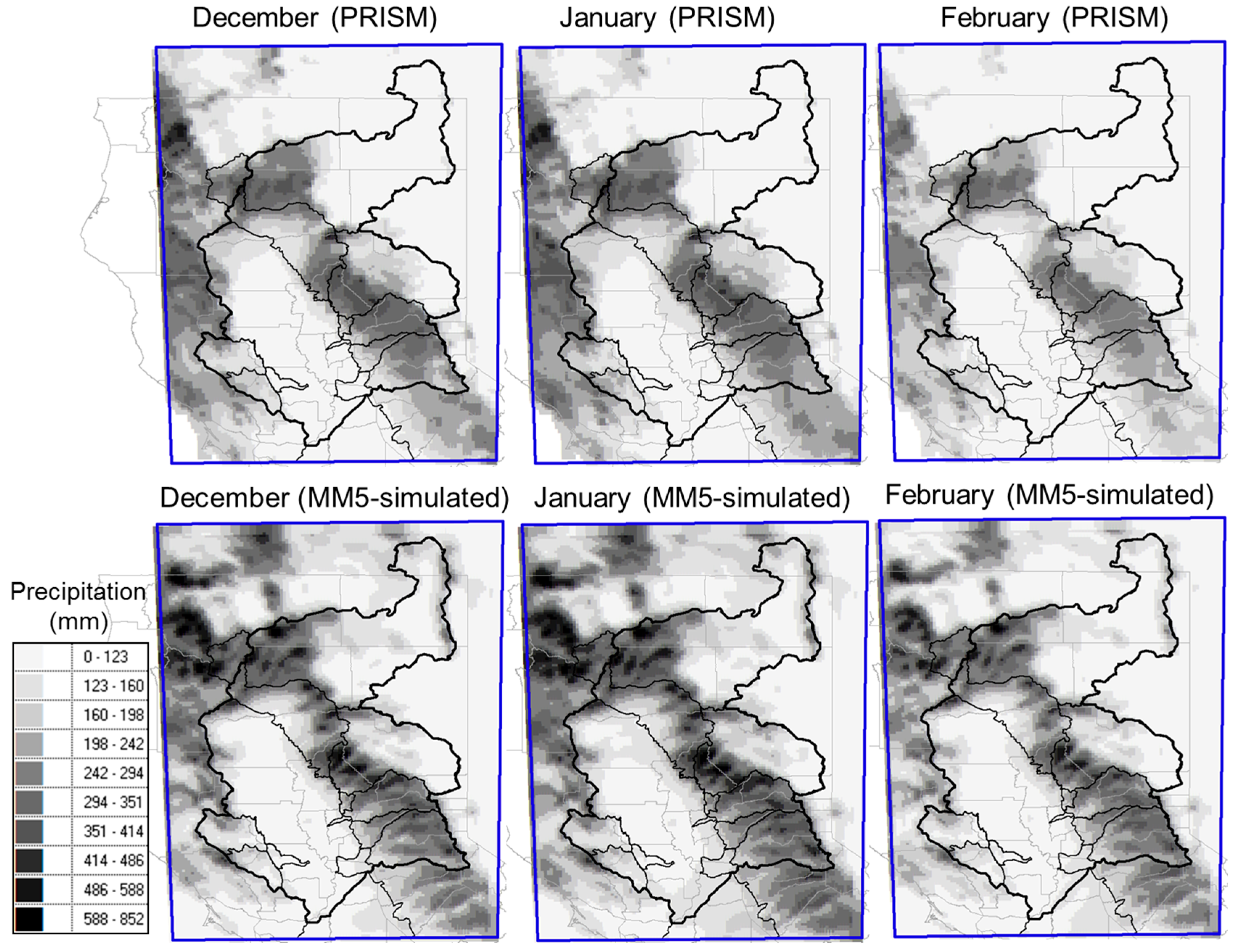
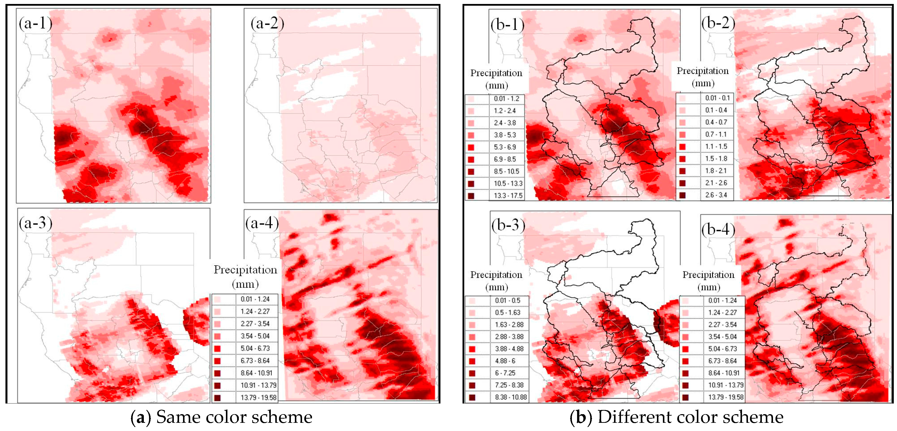
3.3. Evaluation of Spatial Characteristics over the Whole Modeling Domain at Regional Scale

As a key input for models of hydrological processes over a watershed, the spatial characteristics of precipitation fields are important because hydrological processes are locally diverse due to the heterogeneity of the land surface and soil hydraulic properties within a watershed. In this study, the simulated precipitation fields were first compared against PRISM precipitation fields in order to evaluate the spatial distribution of the mean monthly precipitation during 1950–1999 over the whole modeling domain of Northern California.
Figure 6 shows some example comparisons of mean monthly precipitation in December, January, and February between MM5-simulated precipitation and PRISM data over Northern California during 1950–1999. Spatial distributions of mean monthly precipitation by the dynamic downscaling (MM5) from NCAR/NCEP reanalysis data match the PRISM data reasonably well over the simulation domain, especially at low and median elevation ranges. The magnitudes of precipitation along the mountain ridges in the Northwest Coastal region and the Sierra Nevada region in Northern California are slightly higher than the PRISM precipitation. Figure 7 shows basin-average comparisons of mean monthly precipitation between PRISM and MM5-simulated precipitation for eight watersheds in Northern California during 1950–1999. In general, the results in Figure 6 and Figure 7 are similar with respect to the mean monthly comparisons of basin-average precipitation for the eight selected watersheds in Northern California. The basin-average precipitation values are slightly higher at high-elevation watersheds (e.g., TRI, ARW and SHA) but are comparable at low-elevation watersheds (e.g., NCV and CCW).
It is noted that many physiographic and climatic effects were incorporated in the creation of the PRISM precipitation data. As such, this dataset is one of the most reliable and comparable datasets for model calibration or validation. However, the basic assumption in PRISM is that given a homogenous hillslope, precipitation can be predicted through a moving-window regression function with a linear relationship with the elevation. The precipitation generated by PRISM depends on ground observations which are located in similar physiographic and climatic areas. However, ground observations may not be available or may be limited. As such, precipitation comparisons to PRISM data at high elevations may not be appropriate.
For example, TRI is located in a high-elevation mountainous terrain, and it is affected by moisture influx from the Pacific, e.g., atmospheric rivers. In the TRI watershed, 11 ground stations were found from the CDEC CDWR dataset, and most observations since the late 1980s are available with the exception of two stations (CLE and CFF) which are located in valleys. There are no observational stations along the mountain ridges from north to east. Within this framework the MM5-simulated results show the effect of orography on precipitation while PRISM data show a smooth appearance of mean monthly precipitation fields in December during 1950–1999 (Figure 8). Historically, extreme precipitation events begin in late December. Therefore, December has been selected in order to investigate the spatial structures of extreme precipitation in complex terrain.
MM5 simulation results were also compared with NCEP/EMC U.S. Gridded Precipitation products (gauge-only, radar, and Stage IV) in order to evaluate the MM5 atmospheric model–based downscaling performance on reproducing the spatial characteristics of hourly, 24 h and monthly accumulated precipitation fields during December 2005. The precipitation event in December of 2005 is one of the most extreme events which has occurred since the NCEP/EMC U.S. Gridded Precipitation products, including Stage IV datasets, were made available in 2002 [48]. These U.S. Gridded Precipitation products provide sub-monthly precipitation at fine spatial grid scales (about 4 km). The gauge-only data is the NCEP Stage II gauge-based precipitation, which is derived from automated precipitation gauge observations, wherein erroneous gauge data are removed according to a reject-list of apparently faulty gauges. The radar-only product with quality control is created by the WSR-88D Radar Product Generator at each radar site. Each individual radar estimate is merged with other radar estimates on the national Hydrologic Rainfall Analysis Project (HRAP) grid. Radar estimates that fall into the same bin are averaged together within that bin by a simple inverse-distance weighted method. The Stage IV multi-sensor product (Stage IV) combines the precipitation products from the regional hourly/6 h multi-sensor (radar and rain gauge) precipitation analyses, produced by the 12 river forecast centers, with quality control–performed manual NWS forecasts. Therefore, the Stage IV product may be considered to be a reliable reference for precipitation observations. The detailed information on NCEP/EMC U.S. Gridded Precipitation products is available at [48].
Figure 9 shows the spatial comparisons of gauge-only, radar with bias removal and Stage IV observations together with MM5-simulated precipitation fields for the hourly accumulated precipitation fields (6 a.m. GMT on 31 December 2005). Figure 9a,b are the same precipitation fields from each product, but the color schemes for the magnitudes of precipitation are different in order to distinguish the spatial patterns among various products. The radar product shows precipitation magnitudes that are too small for spatial comparison, but the spatial patterns of precipitation are captured well by the radar product. As can be seen in Figure 9a, the spatial distribution of MM5-simulated precipitation is comparable to the Stage IV products, but the radar-only product shows precipitation magnitudes that are too small when compared to the other products. The gauge-only product has a smooth appearance (similar to the distribution of the PRISM precipitation field in Figure 8). On the other hand, the other products show a banded structure for the precipitation fields due to wind and orographic effects (Figure 9). The clearer banded structure in the MM5-simulated results may be due to the grid resolution of the simulation. Although the MM5-simulated results are the closest to the Stage IV product in terms of both the magnitudes and the spatial pattern of precipitation, the Stage IV product has a spatial coverage problem around high-elevation regions such as the Sierra Nevada and the northern coastal regions in California.
Figure 10 shows the spatial comparisons of gauge-only, radar with bias removal, and Stage IV observations together with the corresponding MM5-simulated precipitation fields for the 24 h (Figure 10a) and monthly (Figure 10b) accumulated precipitation fields. From this figure it may be seen that the MM5-simulated precipitation fields are quite similar to the corresponding Stage IV products with respect to the magnitudes and the spatial patterns of precipitation. The gauge-only products show a smoother appearance and less precipitation when compared to MM5-simulated precipitation and the Stage IV estimates, especially for monthly accumulation. However, the banded structure of precipitation fields is no longer seen in the Stage IV products in Figure 10 (24 h and monthly accumulation) because the Stage IV 24 h and monthly products are accumulated from 6 h Stage IV products (not hourly). Meanwhile, the radar product cannot be used in the Stage IV 6 h product estimates due to the spatial coverage problem of the radar product.
The simulated precipitation and wind fields by the MM5 model over the Northern California simulation domain together with the digital elevation model of the domain at (a) 3, (b) 9, (c) 27, and (d) 81 km grid resolutions on (6 a.m. GMT on 31 December 2005) are shown in Figure 11 in order to investigate the effect of banded structures and orographic effects on precipitation with respect to various grid sizes. The time of Figure 11 (6 a.m. GMT on 31 December 2005) is the same as that of Figure 9. It is clearly seen in Figure 11 that the spatial details of the topography are smoothed significantly with the increase in the grid resolutions from the 3 km grid size to the 81 km grid size within the simulation domain. At the 3 km grid resolution (Figure 11a) the spatial details of the topography are described well from low-lying flat areas to high-elevation mountain regions. Those spatial details are described relatively well up to the 9 km grid resolution (Figure 11b). However, the spatial details of the topography, seen at the 3 km and 9 km grid resolutions, are no longer seen at the 27 km grid resolution (Figure 11c) and 81 km grid resolutions (Figure 11d). From these figures it may also be inferred that the precipitation and wind fields are significantly affected by the local topography in terms of their spatial structures and magnitudes. For example, the effects of banded structures and orography on precipitation and wind fields are described well at the 3 km grid resolution (Figure 11a) and at 9 km grid resolution (Figure 11b) while the spatial details of precipitation and wind fields fade away at the 27 km grid (Figure 11c) and 81 km grid (Figure 11d) resolutions.
Since precipitation provides the main source of water for hydrological processes that occur in time and space within a watershed, the spatial variation of precipitation has a fundamental impact on the outcome of hydrological processes within a watershed. Similarly, the wind field over a watershed is an important factor in evapotranspiration processes and in the spatial distribution of snow within a watershed. From the above analysis one may infer that the dynamical downscaling of precipitation and wind to 3 km and 9 km grid resolutions can properly account for the effect of local topography and land cover on the spatial distributions of these climate variables. In turn, such realistic modeling of the precipitation and wind fields would positively impact the hydrologic modeling of streamflow, snow, and evapotranspiration processes within a watershed. Meanwhile, the spatial distributions of precipitation and wind are not well-resolved at 27 km and 81 km grid resolutions. As such, the results of hydrologic modeling that utilizes such coarse-resolution precipitation and wind as inputs may not produce reliable hydrologic process simulation results.

4. Summary and Conclusions

In this study, coarse resolution NCEP/NCAR Reanalysis I precipitation for Northern California (approximately 170,000 km2) was dynamically downscaled to an hourly, 3 km grid resolution using the MM5 atmospheric model over the period 1950–1999. The dynamically downscaled precipitation was then evaluated at point scale, watershed scale and regional scale against corresponding in situ rain gauges and gridded observations. The spatial structures of MM5-simulated hourly, daily and monthly accumulated precipitation fields in December 2005 were also evaluated in order to investigate the effects of banded structures and orography on precipitation fields. This analysis was based on various observations from NCEP/EMC U.S. Gridded Precipitation products (gauge-only, radar, and Stage IV). Additionally, the effect of orography on precipitation and wind fields with respect to horizontal grid sizes (3 km, 9 km, 27 km, and 81 km grids) from four nested grids used for the MM5 simulations was also investigated. From this study the following conclusions may be reached, as detailed below.
From the results of point-scale evaluation based on the precipitation data from eight ground gauges during 1950–1999, the MM5-simulated precipitation values matched the corresponding ground-observed values generally well with respect to the timing as well as the magnitude of monthly precipitation. On scatter plots, the simulated precipitation values were distributed well along the 1:1 lines against the corresponding observed values. For the evaluation at watershed scale, the MM5-simulated precipitation was compared to the PRISM precipitation for eight watersheds (SRW, SHA, TRI, NCV, UFRW, YBW and CCW) in Northern California during 1950–1999. The MM5-simulated basin-average monthly precipitation values provided an excellent match with PRISM-based basin-average precipitation values. The results of the scatter plots showed that the model-simulated and PRISM values are distributed closely along the 1:1 line for all eight watersheds, especially SRW, UFRW, NCV, YBW, and CCW. The mean and the standard deviation of MM5-simulated basin-average precipitation were found to be close to the corresponding mean and standard deviation (STDEV) values from the PRISM data. Also, high values for the coefficient of determination (R2) and for Nash-Sutcliffe efficiency (ENS) statistic were found when model-simulated precipitation was compared against PRISM data for the eight selected watersheds in Northern California.
Although, in general, the spatial distributions of the MM5-simulated mean monthly precipitation fields matched well against the corresponding PRISM precipitation fields during 1950–1999, the MM5-simulated values were slightly higher at the high-elevation mountain areas than the corresponding PRISM data. This may be due to PRISM precipitation values being based on the ground observations which are generally located at low-elevation areas near roads or around residential areas in order to be operationally accessible. As such, the spatial structures of the MM5-simulated precipitation fields were evaluated further based on various grid-based observation fields from NCEP/EMC U.S. Gridded Precipitation products (gauge-only, radar, and Stage IV). In this further investigation, the radar products showed much smaller precipitation magnitudes than other products (gauge-only, Stage IV), but the radar products described the banded precipitation structures and the orographic effects on precipitation well. The gauge-based precipitation fields did not capture the banded precipitation structures and orographic effects on precipitation, and showed a spatially smooth precipitation appearance (similar to the PRISM precipitation fields) over Northern California. The MM5-simulated precipitation fields showed spatial structures that are similar to those from radar and Stage IV products, and showed precipitation magnitudes similar to those from gauge-only and Stage IV products over Northern California. Therefore, one may conclude that MM5 simulations can capture not only the banded precipitation structures and orographic effects on precipitation but also the magnitudes of precipitation quite well over Northern California.
From the results of the spatial comparisons of topography, precipitation and wind fields with respect to various grid sizes, it was found that the spatial distributions of the modeled precipitation and wind fields over Northern California are significantly impacted by the variation in the model grid resolutions. The grid resolutions of 3 km and 9 km resolve the local topography well, yielding realistic spatial patterns for precipitation and wind. However, the 27 km and 81 km grid sizes could not resolve the local topography, and, hence, could not resolve the spatial variation of precipitation and wind fields over Northern California.
In conclusion, in this study the performance of dynamically downscaled precipitation from NCEP/NCAR reanalysis data was evaluated at point scale, watershed scale and spatial scale against corresponding ground observations, PRISM data, and NCEP/EMC U.S. Gridded Precipitation products. Also, the spatial characteristics of the simulated precipitation and wind fields with respect to various grid sizes were investigated in order to gain insight to the topographic effect on the atmospheric state variables. The results of this study indicate that the MM5 regional atmospheric model can dynamically downscale the climate variables from the synoptic-scale products such as reanalysis data to a finer grid scale satisfactorily, while also quantifying the effect of the topography and land cover on atmospheric information.

Acknowledgments

This work is partially supported by the Korea Agency for Infrastructure Technology Advancement (KAIA) grant funded by the Ministry of Land, Infrastructure and Transport (Grant 17AWMP-B0830660-04).

Author Contributions

Z. Q. Chen set up the regional climate model; Noriaki Ohara, Suhyung Jang and Shuichi Kure reconstructed and simulated the atmospheric and hydrological data; Toan Trinh collected the observations; Suhyung Jang and Kei Ishida analyzed and wrote the paper with support from M. Levent Kavvas, Michael L. Anderson, G. Matanga, and Kara J. Carr.

Conflicts of Interest

The authors declare no conflict of interest.

References

  1. Kalnay, E.; Kanamitsu, M.; Kistler, R.; Collins, W.; Deaven, D.; Gandin, L.; Iredell, M.; Saha, S.; White, G.; Woollen, J.; et al. The NCEP/NCAR 40-Year Reanalysis Project. Bull. Am. Meteorol. Soc. 1996, 77, 437–471. [Google Scholar] [CrossRef]
  2. Kavvas, M.L.; Kure, S.; Chen, Z.Q.; Ohara, N.; Jang, S. WEHY-HCM for Modeling Interactive Atmospheric-Hydrologic Processes at Watershed Scale. I: Model Description. J. Hydrol. Eng. 2013, 18, 1262–1271. [Google Scholar] [CrossRef]
  3. Kure, S.; Jang, S.; Ohara, N.; Kavvas, M.L.; Chen, Z.Q. WEHY-HCM for Modeling Interactive Atmospheric-Hydrologic Processes at Watershed Scale. II: Model Application to Ungauged and Sparsely Gauged Watersheds. J. Hydrol. Eng. 2013, 18, 1272–1281. [Google Scholar] [CrossRef]
  4. Grotch, S.L.; MacCracken, M.C. The Use of General Circulation Models to Predict Regional Climatic Change. J. Clim. 1991, 4, 286–303. [Google Scholar] [CrossRef]
  5. Fowler, H.J.; Blenkinsop, S.; Tebaldi, C. Linking climate change modelling to impacts studies: Recent advances in downscaling techniques for hydrological modelling. Int. J. Climatol. 2007, 27, 1547–1578. [Google Scholar] [CrossRef]
  6. Christensen, J.H.; Christensen, O.B. Climate modelling: Severe summertime flooding in Europe. Nature 2003, 421, 805–806. [Google Scholar] [CrossRef] [PubMed]
  7. Maraun, D.; Wetterhall, F.; Ireson, A.M.; Chandler, R.E.; Kendon, E.J.; Widmann, M.; Brienen, S.; Rust, H.W.; Sauter, T.; Themeßl, M.; et al. Precipitation downscaling under climate change: Recent developments to bridge the gap between dynamical models and the end user. Rev. Geophys. 2010, 48, RG3003. [Google Scholar] [CrossRef]
  8. Jang, S.; Kavvas, M.L. Downscaling global climate simulations to regional scales: Statistical downscaling versus dynamical downscaling. J. Hydrol. Eng. 2015, 20. [Google Scholar] [CrossRef]
  9. Kavvas, M.L.; Chen, Z.Q.; Tan, L.; Soong, S.-T.; Terakawa, A.; Yoshitani, J.; Fukami, K. A regional-scale land surface parameterization based on areally-averaged hydrological conservation equations. Hydrol. Sci. J. 1998, 43, 611–631. [Google Scholar] [CrossRef]
  10. Shrestha, R.; Tachikawa, Y.; Takara, K. Input data resolution analysis for distributed hydrological modeling. J. Hydrol. 2006, 319, 36–50. [Google Scholar] [CrossRef]
  11. Haltas, I.; Kavvas, M.L. Scale Invariance and Self-Similarity in Hydrologic Processes in Space and Time. J. Hydrol. Eng. 2011, 16, 51–63. [Google Scholar] [CrossRef]
  12. Diaz-Nieto, J.; Wilby, R.L. A comparison of statistical downscaling and climate change factor methods: Impacts on low flows in the River Thames, United Kingdom. Clim. Chang. 2005, 69, 245–268. [Google Scholar] [CrossRef]
  13. Mearns, L.O.; Giorgi, F.; Whetton, P.; Pabon, D.; Hulme, M.; Lal, M. Guideline for Use of Climate Scenarios Developed from Regional Climate Model Experiments; Data Distribution Centre of the Intergovernmental Panel on Climate Change Task Group on Data and Scenario Support for Impact and Climate Analysis: Geneva, Switzerland, 2003. [Google Scholar]
  14. Jones, R.G.; Murphy, J.M.; Noguer, M. Simulation of climate change over europe using a nested regional-climate model. I: Assessment of control climate, including sensitivity to location of lateral boundaries. Q. J. R. Meteorol. Soc. 1995, 121, 1413–1449. [Google Scholar] [CrossRef]
  15. Frei, C.; Christensen, J.H.; Déqué, M.; Jacob, D.; Jones, R.G.; Vidale, P.L. Daily precipitation statistics in regional climate models: Evaluation and intercomparison for the European Alps. J. Geophys. Res. 2003, 108. [Google Scholar] [CrossRef]
  16. Christensen, J.H.; Christensen, O.B. A summary of the PRUDENCE model projections of changes in European climate by the end of this century. Clim. Chang. 2007, 81, 7–30. [Google Scholar] [CrossRef]
  17. Fowler, H.J.; Kilsby, C.G.; O’Connell, P.E.; Burton, A. A weather-type conditioned multi-site stochastic rainfall model for the generation of scenarios of climatic variability and change. J. Hydrol. 2005, 308, 50–66. [Google Scholar] [CrossRef]
  18. Frei, C.; Schöll, R.; Fukutome, S.; Schmidli, J.; Vidale, P.L. Future change of precipitation extremes in Europe: Intercomparison of scenarios from regional climate models. J. Geophys. Res. 2006, 111, D06105. [Google Scholar] [CrossRef]
  19. Murphy, J. An Evaluation of Statistical and Dynamical Techniques for Downscaling Local Climate. J. Clim. 1999, 12, 2256–2284. [Google Scholar] [CrossRef]
  20. Leung, L.R.; Qian, Y.; Bian, X. Hydroclimate of the Western United States Based on Observations and Regional Climate Simulation of 1981–2000. Part I: Seasonal Statistics. J. Clim. 2003, 16, 1892–1911. [Google Scholar] [CrossRef]
  21. Leung, L.R.; Qian, Y.; Bian, X.; Hunt, A. Hydroclimate of the Western United States Based on Observations and Regional Climate Simulation of 1981–2000. Part II: Mesoscale ENSO Anomalies. J. Clim. 2003, 16, 1912–1928. [Google Scholar] [CrossRef]
  22. Leung, L.R.; Qian, Y. Atmospheric rivers induced heavy precipitation and flooding in the western U.S. simulated by the WRF regional climate model. Geophys. Res. Lett. 2009, 36. [Google Scholar] [CrossRef]
  23. Rauscher, S.A.; Coppola, E.; Piani, C.; Giorgi, F. Resolution effects on regional climate model simulations of seasonal precipitation over Europe. Clim. Dyn. 2010, 35, 685–711. [Google Scholar] [CrossRef]
  24. Liu, J.; Bray, M.; Han, D. Sensitivity of the Weather Research and Forecasting (WRF) model to downscaling ratios and storm types in rainfall simulation. Hydrol. Process. 2012, 26, 3012–3031. [Google Scholar] [CrossRef]
  25. Leung, L.R.; Qian, Y.; Bian, X.; Washington, W.M.; Han, J.; Roads, J.O. Mid-Century Ensemble Regional Climate Change Scenarios for the Western United States. Clim. Chang. 2004, 62, 75–113. [Google Scholar] [CrossRef]
  26. Salathé, E.P.; Steed, R.; Mass, C.F.; Zahn, P.H. A High-Resolution Climate Model for the U.S. Pacific Northwest: Mesoscale Feedbacks and Local Responses to Climate Change. J. Clim. 2008, 21, 5708–5726. [Google Scholar] [CrossRef]
  27. Salathé, E.P.; Leung, L.R.; Qian, Y.; Zhang, Y. Regional climate model projections for the State of Washington. Clim. Chang. 2010, 102, 51–75. [Google Scholar] [CrossRef]
  28. Gao, Y.; Leung, L.R.; Lu, J.; Liu, Y.; Huang, M.; Qian, Y. Robust spring drying in the southwestern U.S. and seasonal migration of wet/dry patterns in a warmer climate. Geophys. Res. Lett. 2014, 41, 1745–1751. [Google Scholar] [CrossRef]
  29. Caldwell, P.; Chin, H.-N.S.; Bader, D.C.; Bala, G. Evaluation of a WRF dynamical downscaling simulation over California. Clim. Chang. 2009, 95, 499–521. [Google Scholar] [CrossRef]
  30. Gao, Y.; Fu, J.S.; Drake, J.B.; Liu, Y.; Lamarque, J.-F. Projected changes of extreme weather events in the eastern United States based on a high resolution climate modeling system. Environ. Res. Lett. 2012, 7, 044025. [Google Scholar] [CrossRef]
  31. Bachner, S.; Kapala, A.; Simmer, C. Evaluation of daily precipitation characteristics in the CLM and their sensitivity to parameterizations. Meteorol. Z. 2008, 17, 407–419. [Google Scholar] [CrossRef]
  32. Fowler, H.J.; Ekström, M. Multi-model ensemble estimates of climate change impacts on UK seasonal precipitation extremes. Int. J. Climatol. 2009, 29, 385–416. [Google Scholar] [CrossRef]
  33. Tatsumi, K.; Yamashiki, Y.; Takara, K. Effect of uncertainty in temperature and precipitation inputs and spatial resolution on the crop model. Hydrol. Res. Lett. 2011, 5, 52–57. [Google Scholar] [CrossRef]
  34. Nakaegawa, T.; Nakakita, E. Comment on “Effect of uncertainty in temperature and precipitation inputs and spatial resolution on the crop model” by Kenichi Tatsumi, Yosuke Yamashiki and Kaoru Takara. Hydrol. Res. Lett. 2012, 6, 13–14. [Google Scholar] [CrossRef]
  35. California Data Exchange Center (CDEC). Available online: http://cdec.water.ca.gov/ (accessed on 10 August 2017).
  36. National Elevation Dataset (NED). Available online: https://nationalmap.gov/elevation.html (accessed on 10 August 2017).
  37. Global Land Cover Characteristics (GLCC) Data Base Version 2.0. Available online: https://lta.cr.usgs.gov/glcc/globdoc2_0 (accessed on 10 August 2017).
  38. Grell, G.A.; Dudhia, J.; Stauffer, D. A Description of the Fifth-Generation Penn State/NCAR Mesoscale Model (MM5); Mesoscale and Microscale Meteorology Division, National Center for Atmospheric Research: Boulder, CO, USA, 1994; p. 121. [Google Scholar]
  39. NCAR/NCEP Reanalysis I Data. Available online: http://rda.ucar.edu/datasets/ds090.1/ (accessed on 10 August 2017).
  40. Giorgi, F.; Gutowski, W.J. Regional downscaling and the CORDEX initiative. Ann. Rev. Environ. Resour. 2015, 40, 467–490. [Google Scholar] [CrossRef]
  41. Grubišić, V.; Vellore, R.K.; Huggins, A.W. Quantitative Precipitation Forecasting of Wintertime Storms in the Sierra Nevada: Sensitivity to the Microphysical Parameterization and Horizontal Resolution. Mon. Weather Rev. 2005, 133, 2834–2859. [Google Scholar] [CrossRef]
  42. Reeves, H.D.; Lin, Y.-L.; Rotunno, R. Dynamic Forcing and Mesoscale Variability of Heavy Precipitation Events over the Sierra Nevada Mountains. Mon. Weather Rev. 2008, 136, 62–77. [Google Scholar] [CrossRef]
  43. Ohara, N.; Kavvas, M.L.; Kure, S.; Chen, Z.Q.; Jang, S.; Tan, E. Physically Based Estimation of Maximum Precipitation over American River Watershed, California. J. Hydrol. Eng. 2011, 16, 351–361. [Google Scholar] [CrossRef]
  44. Ishida, K.; Kavvas, M.L.; Jang, S.; Chen, Z.Q.; Ohara, N.; Anderson, M.L. Physically Based Estimation of Maximum Precipitation over Three Watersheds in Northern California: Atmospheric Boundary Condition Shifting. J. Hydrol. Eng. 2015, 20, 04014052. [Google Scholar] [CrossRef]
  45. Ishida, K.; Kavvas, M.L.; Jang, S. Comparison of Performance on Watershed-Scale Precipitation between WRF and MM5. Am. Soc. Civ. Eng. 2015, 989–993. [Google Scholar] [CrossRef]
  46. Skamarock, W.C.; Klemp, J.B.; Dudhia, J.; Gill, D.O.; Barker, D.M.; Wang, W.; Powers, J.G. A Description of the Advanced Research WRF Version 2; Mesoscale and Microscale Meteorology Division, National Center for Atmospheric Research: Boulder, CO, USA, 2005; p. 88. [Google Scholar]
  47. PRISM Preciptation Data. Available online: http://prism.oregonstate.edu (accessed on 10 August 2017).
  48. NCEP/EMC U.S. Gridded Precipitation. Available online: http://data.eol.ucar.edu/ (accessed on 10 August 2017).
  49. Daly, C.; Halbleib, M.; Smith, J.I.; Gibson, W.P.; Doggett, M.K.; Taylor, G.H.; Curtis, J.; Pasteris, P.P. Physically sensitive mapping of climatological temperature and precipitation across the conterminous United States. Int. J. Climatol. 2008, 28, 2031–2064. [Google Scholar] [CrossRef]
Figure 1. Study area and simulation domain (latter highlighted by the blue box). Shaded areas indicate the eight selected watersheds and circles mark the locations of the eight observation stations used in this study. Abbreviations to eight watersheds are provided in the main text and Table 1.
Sustainability 09 01457 g001
Figure 2. Digital elevation model (left) from U.S. Geological Survey (USGS) 2 arc-second grid spacing data [36] and Land use/land cover types (right) from Global Land Cover Characteristics (GLCC) data version 2 from USGS [37] over the study area.
Sustainability 09 01457 g002
Figure 3. Regional hydro-climate model (MM5) simulation domains for the study area.
Sustainability 09 01457 g003
Figure 4. Scatter plots of the ground observed precipitation against the MM5-simulated (NCEP) precipitation at eight ground stations during 1950–1999.
Sustainability 09 01457 g004
Figure 5. Scatter plots of basin-average precipitation between PRISM and MM5-simulated precipitation for eight Northern California watersheds during 1950–1999.
Sustainability 09 01457 g005
Figure 6. Example spatial comparisons for the mean monthly precipitation (December, January, and February) between PRISM and MM5-simulated precipitation during 1950–1999.
Sustainability 09 01457 g006
Figure 7. Basin-average comparisons of mean monthly precipitation between PRISM (grey block) and MM5-simulated (white block) precipitation for eight watersheds in Northern California during 1950–1999.
Sustainability 09 01457 g007
Figure 8. Example spatial comparisons of mean monthly precipitation in December between PRISM and MM5-simulated precipitation for TRI during 1950–1999 with the location of 11 ground stations in the CDEC DWR dataset (DEM = Digital Elevation Model).
Sustainability 09 01457 g008
Figure 9. Spatial comparisons of hourly accumulated precipitation fields at 6 a.m. GMT on 31 December 2005 from gauge-only (a-1,b-1), radar with bias removal (a-2,b-2), and Stage IV (a-3,b-3) observations, together with NCEP/NCAR-based MM5 simulations (a-4,b-4).
Sustainability 09 01457 g009
Figure 10. Spatial comparisons of (a) 24 h (1 p.m. GMT on 30 December 2005—12 p.m. GMT on 31 December 2005) and (b) one-month (1 p.m. GMT on 1 December 2005—12 p.m. GMT on 1 January 2006) accumulated precipitation fields from gauge-only (a-1,b-1), radar with bias removal (a-2,b-2), and Stage IV (a-3,b-3) observations together with NCEP/NCAR-based MM5 simulations (a-4,b-4).
Sustainability 09 01457 g010
Figure 11. The simulated precipitation and wind fields by MM5 over the Northern California simulation domain together with the digital elevation model of the domain at (a) 3, (b) 9, (c) 27, and (d) 81 km grid resolution at 6 a.m. GMT on 31 December 2005. The contour map shows precipitation fields; the vector map shows wind fields; the 3D color map shows the digital elevation model for each grid resolution (3, 9, 27 and 81 km).
Sustainability 09 01457 g011
Table 1. Summary information on watersheds and ground observational stations selected for this study. The eight ground observation stations are from the California Data Exchange Center (CDEC, [35]) of the California Department of Water Resources (CDWR).
WatershedGround Observationa
IDBasin NameDrainage Area (km2)Mean Elevation (m)IDStation NameElevation (m)
SRWSacramento River71,721921SHOShasta dam328
SHAShasta dam19,8181419WVRWeaverville RS625
TRITrinity dam17011417GNVGreenville RS1088
NCVNorthern Central Valley27,351197BOWBowman1641
UFRWUpper Feather River92251532CLFColfax732
ARWAmerican River55351149ORLOrland77
YBWYuba River35281202UKHUkiah193
CCWCache Creek2970535DVSDavis 2WSW18
Table 2. Statistical comparisons of MM5-simulated (NCEP) versus PRISM precipitation during 1950–1999.
WatershedModelMean (mm)STDEV (mm)RMSE (mm)R2Nash-Sutcliffe Efficiency
SRWPRISM79.6391.57
MM5-simulated88.20104.7032.720.920.87
SHAPRISM71.5672.84
MM5-simulated97.60100.2248.940.870.55
TRIPRISM128.91153.14
MM5-simulated155.57193.1079.070.870.73
NCVPRISM50.9263.78
MM5-simulated53.6674.1125.150.890.83
UFRWPRISM100.52120.76
MM5-simulated106.17125.7939.290.900.89
ARWPRISM101.59121.49
MM5-simulated114.85152.4757.540.890.78
YBWPRISM136.31165.91
MM5-simulated140.50180.4156.270.900.88
CCWPRISM72.1697.28
MM5-simulated65.7795.7531.180.900.90

