
Analysis and Prediction of Changes in Coastline Morphology in the Bohai Sea, China, Using Remote Sensing


1
School of Geology and Geomatics, Tianjin Chengjian University, Jinjing Road, Tianjin 300384, China
2
College of Global Change and Earth System Science, Beijing Normal University, Beijing 100875, China
*
Author to whom correspondence should be addressed.
Sustainability 2017, 9(6), 900; https://doi.org/10.3390/su9060900
Submission received: 1 April 2017
/
Revised: 22 May 2017
/
Accepted: 22 May 2017
/
Published: 29 May 2017
Abstract
:Coastline change reflects the dynamics of natural processes and human activity, and influences the ecology and environment of the coastal strip. This study researched the change in coastline and sea area of the Bohai Sea, China, over a 30-year period using Landsat TM and OLI remote sensing data. The total change in coastline length, sea area, and the centroid of the sea surface were quantified. Variations in the coastline morphology were measured using four shape indexes: fractal dimension, compact ratio, circularity, and square degree. Equations describing fit of the shape index, coastline length, and marine area were built. Then the marine area 10 years later was predicted using the model that had the highest prediction accuracy. The results showed that the highest prediction accuracy for the coastline length was obtained using a compound function. When a cubic function was used to predict the compact ratio, then the highest prediction accuracy was obtained using this compact ratio and a quadratic function to predict sea area. This study can provide theoretical support for the coastal development planning and ecological environment protection around the Bohai Sea.
1. Introduction
Coastline is physical interface of land and ocean. Changes in coastline occur for two main reasons: natural processes and human factors. Cities and populations in coastal areas have increased rapidly due to abundant natural resources, leading to numerous development projects. Coastal development has brought prosperity to society but also has led to coastal hazards such as erosion by the sea, sea water intrusion, coral bleaching, and coastline change [1]. Coastline change in turn affects coastal ecological environment and economic development and wellbeing of communities. Coastline change reflects modification of the natural environment and influence of human activities in coastal areas, so research on the spatial and temporal patterns of coastline change is of great significance.
Wavelet analysis was extremely useful as a tool for analyzing coastal data and for data-driven modelling. However, there are still limits in scales, space, and time to its use [2,3]. Remote sensing has characteristics of broad scale, rapid, and real-time collection, which can capture environmental dynamics in many situations. Using remote sensing to analyze coastline changes can provide dynamic, scientific, timely, and valid information for relevant decision-making departments, and can assist with not only development and use of the coast as well as tidal flats but also with disaster evaluation of the ocean. At present, remote sensing is the main method of monitoring coastline changes [4,5]. Al-Hatrushi monitored the coastline change of the Al Hawasnah tidal inlet on the Al Batinah coast of the Sultanate of Oman using remote sensing and GIS [6]. Deepika et al. estimated and forecasted the rate of coastline change using remote sensing [7], while Zhang et al. evaluated coastline changes due to human intervention in the Zhoushan Islands of China [8]. Landsat TM and OLI remote sensing data are often used in the study of coastlines because it is easily obtained and has a long temporal coverage. For example, Bouchahma and Yan used eight Landsat TM images to develop an approach to measure, analyze, and model the coastline, then predict and manage the changes in the coastal environment [9]. Kankara et al. estimated long and short term coastline changes along Andhra Pradesh coast using TM remote sensing images [10]. Cui et al. studied the coastal landform, coastline, and erosion of geomorphic silt in Laizhou Bay over the past 30 years using TM and OLI data [11]. Wu et al. used multi-year TM and OLI images to analyze temporal and spatial variation and driving forces of coastline change in Yueqing Bay [12].
The Bohai Sea plays an important role in China, including in the fields of energy production, environment protection, and economic development. Most studies to date have examined parts of the Bohai Sea coast, but few have carried out a comprehensive analysis of the whole Bohai Sea. For example, Li et al. studied the temporal and spatial variation of the coastline and coastal zone of the Bohai Bay in five key research areas [13]. Zhang et al. studied the evolution of coastline and tidal flats of the western and southern parts of the Bohai Bay from 1975 to 2010 and identified factors that affected these changes [14]. Sun et al. studied the location, length, and structure of the Bohai Bay coastline from 2000 to 2010, carried out a quantitative inversion of the space-time change process of the coastline, and analyzed its causes [15]. Zhang et al. extracted and monitored coastline change in the Qinhuangdao City [16]. Wang et al. researched the process of morphological changes in coastline and near-shore marine areas on two sides of the Port of Huanghua [17].
Broadly, the instantaneous water line is the direct boundary between ocean and land, thus it can be considered to be the shoreline. At present, the shoreline is generally replaced by water edge of the imaging time when monitoring the change of coastline using remote sensing [18]. The coastline extraction methods are generally divided into automatic extraction, semi-automatic extraction, and visual interpretation. Image noise and resolution factor will influence the continuity and correctness of coastline when using automatic and semi-automatic extraction methods, as such, the extraction results need to be modified by artificial auxiliary [19]. Unified interpretation signs shall be established according to different coastline types and a comparatively accurate result can be obtained using a visual interpretation method. This method is suitable for research of large-scale shoreline change, for example, Miao et al. used the visual interpretation method to extract coastline in the Tumen River estuary and adjacent areas and monitor its change of nearly 30 years [20]. Zhang used the visual interpretation method to obtain such information as location, length, and type of Zhuhai coastline and did detailed analysis and research on the change of coastline between 2004 and 2014 [21]. Liao et al. extracted coastline information of Zhejiang province using the visual interpretation method and analyzed the spatial and temporal variation characteristics [22].
This paper aims to study the basic situation, change rule, and trend of the Bohai Sea coastline. It can meet the research requirements to regard the instantaneous water edge as the coastline. The coastline was divided into artificial coast, bedrock coast, sandy coast, and muddy coast according to remote sensing image information and the actual situation. The coastline was extracted using the visual interpretation method based on establishing various interpretation signs of different types of coastlines. The length of the coastline, sea area and the change of the centroid of the Bohai Sea were obtained for four years (1985, 1995, 2005, and 2015). The changes in the coastlines of three adjacent coastal provinces, one city, and 46 counties over the 30-year period were analyzed. The changes in coastline morphology were studied using four shape indexes: fractal dimension, compact ratio, circularity, and square degree. The best fitting models for each shape index in relation to coastline length, and between each shape index and the year were built by comparing the coefficients of determination. The fitting models for compact ratio, circularity, and square degree in relation to coastline length were hardly mentioned in the previous studies. Finally, the scheme used to forecast changes in the coastline and sea area in the next 10-year period was built, and an evaluation of the forecasted results was carried out.
2. Study Area and Data
The Bohai Sea is located at 37°27′–41°0′N, 117°35′–121°10′E [23] (Figure 1). The eastern end of the Bohai Sea and Yellow Sea are linked by the Bohai straits. The Bohai Sea has a variety of marine species, and is used to provide five economic resources: fishing, ports, oil, tourism, and sea salt. It has experienced pollution from the land and oil spills. In recent years, with rapid economic growth, the Circum-Bohai Sea Economic Zone has become one of the most important areas for economic development in China after the Pearl River delta and the Yangtze River delta [24]. In order to study coastline changes over the whole Bohai Sea during 1985–2015, this study used Landsat5 TM remote sensing images in 1985, 1995, and 2005 and Landsat8 OLI remote sensing images in 2015. Seven images were used for each year, and all images included seven bands and the spatial resolution was 30 m after preprocessing. The specific information of the images is shown in Table 1. As beach width naturally fluctuates on a seasonal basis, the best approach is to utilize only imagery from the same season. A uniform coordinate grid system must be chosen so that all maps and air photos can be properly aligned. [25]. As such, all images were from summer and used the same coordinate system: WGS_1984_UTM_Zone_50N.
3. Methods
The methods used in this paper are shown in Figure 2. First, the coastline of the Bohai Sea in 1985, 1995, 2005, and 2015 was digitized, and the change in the total length of coastline, the sea area, and the centroid of the sea surface in four periods: 1985–1995, 1995–2005, 2005–2015, and 1985–2015 were calculated. The degree of change in the coastline was expressed by the percentage of the coastline length in a given period and of the total length in the starting year. After digitization, the coastline was divided into sections using vector data on the national administrative divisions to obtain the coastline length of the three provinces, one municipality directly under the Central Government, and 46 counties (Table 2) adjacent to the Bohai Sea. Then the coastline changes of these regions were analyzed, so that differences in the coastal modification of each county could be identified.
The coastline morphological changes were reflected by four shape indexes: fractal dimension (D), compact ratio (C), circularity (R), and square degree (S). The shape indexes were computed by the perimeter (P) of the Bohai Sea, the sea area (A), the perimeter of the equal area circle (P1) and the perimeter of the equal area square (P2), and computation formulas are as follows [26,27,28]:
The fractal dimension is a good parameter representing coastline characteristics, and has been often used in the study of coastlines [29,30]. The bigger the fractal dimension value, the more complex is the shape of the coastline. As an example, the fractal dimension value of a straight line would be 1, and that of a rectangle would be 2 [31]. The greater the value of the compact ratio, the more compact its shape. The compact ratio is often used to study urban morphology changes, and has proved effective in evaluating the compact degree of urban morphology. Like urban areas, the sea area is complex and irregular, so the compact ratio can also be used to evaluate changes in coastline morphology effectively. Circularity is obtained by dividing the perimeter of an equal area circle by the perimeter of the plane figure, and the square degree is obtained by dividing the perimeter of the equal area quadrate by the perimeter of the plane figure. The circularity score represents the similarity between the shape and a circle. A value of 1 represents a shape that is very close to a circle; higher values indicate more irregular shapes. In the process of coastline change, for example, while the overall shape of the sea surface does not easily change, some parts of the natural smooth coastline tend to become tortuous due to artificial modification. In this case, the circularity score becomes larger. The square degree is comparable to the circularity. It reflects the similarity between the shape and a square. The greater the value, the more irregular is the shape. Artificial coastal construction tends to cause the square degree to become larger compared with the natural coastline. These four shape indexes were chosen to study the morphological changes of coastline.
After the four shape indexes for each of the four periods were obtained, we fitted six types of function models (linear, logarithmic, polynomial, compound, cubic, and power function) by using the coastline length and sea area as the dependent variables and the shape indexes as independent variables. The best fitting model was chosen by comparing the decision coefficients of each model. Multivariate regression was used to contrast with the simple regression mentioned above. The year was used as the dependent variable, and the four shape indexes and coastline length were used as independent variables. Finally, the most suitable model was used to predict the length of the coastline and sea area in 2025.
4. Results
4.1. Coastal Change in the Bohai Sea
Changes in the coastline length and sea area of the Bohai Sea between 1985–1995, 1995–2005, 2005–2015, and 1985–2015 are shown in Table 3. From 1985 to 2015, the coastline length progressively increased, as did the rate of change, while the sea area declined. Compared to the coastline length in 1985, by 2015 the length had increased to a total of 2080.80 km, 73.43% longer than that in 1985. The sea area in 2015 was 2113.33 km2, 2.44% less than that in 1985. The amount of change between 1985 and 1995 was not large: the coastline increased by 1.59%, and the sea area reduced by 0.32%. Between 2005 and 2015, the amount of change was much larger, as the coastline increased by 41.0% and the sea area reduced by 2.0%.
A centroid refers to an imaginary point around which a value is focused. The sea surface after digitization was a homogeneous polygon so the centroid would be determined by the greatest area. Over the 30-year period, the centroid position of the whole Bohai Sea moved about 1.14 km to the southeast (Table 4). Similarly, the centroid moved to the southeast during the periods of 1985–1995 and 2005–2015. This showed that the sea area in the northwest of the Bohai Sea had reduced more or faster than in the southeast. However, the centroid moved to the southwest during 1995–2005, because the sea area in the northwest had reduced more or faster than in the southeast during this decade.
4.2. Coastline Change in the Bohai Sea-Adjacent Coastal Provinces, Cities, and Counties
The coastline length of the adjacent three provinces, one city, and 46 counties to the Bohai Sea in each period are shown in Figure 3. The provincial units and counties which had the largest percentage of change in each interval are shown in Table 5. Overall, during the period from 1985 to 2015, the provincial unit that had the largest percentage of change in coastline length was Tianjin City. Its coastline length increased by 334.01 km, approximately 273.80% of the total length in 1985. The second largest increase occurred in Hebei Province, and its coastline length increased by 480.10 km, approximately 132.64% of the total length in 1985. The coastlines in the Shandong Province and Liaoning Province increased by 682.66 km (75.57%) and 584.03 km (40.37%), respectively. The counties which had the largest percentage of changes in the Shandong Province, Hebei Province, Tianjin City, and Liaoning Province were Wudi County, Huanghua City, Tanggu District, and Bayuquan District, respectively. The change in their coastline lengths were 93.33 km, 165.09 km, 239.78 km, and 77.34 km, respectively, approximately 310.23%, 329.32%, 297.45%, and 230.22% of their lengths in 1985.
From 1985 to 1995, Tianjin City’s coastline length showed the most change among all the provincial units. The counties that had the largest variation were Changyi City (Shandong Province), Luannan County (Hebei Province), Dagang District (Tianjin City), and Linghai City (Liaoning Province). From 1995 to 2005, Hebei Province’s coastline length changed the most among the provincial units. The counties that had the largest variation were Zhanhua County (Shandong Province), Tanghai County (Hebei Province), Dagang District (Tianjin City), and Bayuquan District (Liaoning Province). From 2005 to 2015, Tianjin City’s coastline length had the greatest change among the provincial units. The counties with the largest variations were Wudi County (Shandong Province), Fengnan District (Hebei Province), Hangu District (Tianjin City), and Gaizhou City (Liaoning Province).
The interval distributions of change for the counties within each provincial unit are shown in Table 6. The number of counties that had more than 30% changes in each province progressively increased in each 10-year period. This showed that the area of coastline change had been increasing, which reflected the growing coastal human activities. During the past 30 years, coastlines in the three districts in Tianjin City adjacent to the Bohai Sea all changed more than 200%. The results showed that, at a province level, the biggest amount of change occurred in Tianjin City; while relatively little change occurred in Liaoning Province.
The changes in coastline morphology are influenced by human activities and natural factors, such as coastal sediment, wind, and tides [32]. However, significant changes in a coastline over a period of decades tend to reflect human influences [33]. This paper selected several typical areas of change, as shown in Figure 4, Figure 5 and Figure 6. These were Tianjin City, Tanghai County, Fengnan District, and Huanghua City of Hebei Province. Predominant geological locations and proximity to important coastal developments were the common point of the study areas. The port of Tianjin in the east of Tanggu District is the largest trading port in northern China, and trades goods to many countries in the world. As such, Tanggu District continues to develop very rapidly. Tanghai County (renamed Caofeidian District after 2012), located in the heartland of the Bohai Bay, is the strategic center of coordinated development for the BTT (Beijing-Tianjin-Tangshan) region. Fengnan District is located in the hinterland of the Bohai Economic Rim. The Port of Huanghua is the leading zone of the national trans-century Shenhua project.
4.3. Changes in Coastline Morphology
The results of the four shape indexes for the Bohai Sea in 1985, 1995, 2005, and 2015 were shown in Table 7. From 1985 to 2015, the fractal dimension, circularity, and square degree increased gradually, while the compact ratio became smaller. The economic development over the years changed more and more rock, silt, and sandy coasts into artificial coasts such as salt pans and ports, increasing the morphological complexity of the coastline.
4.4. Model Fit and Prediction
To study the change rule and trend of the coastline, this paper selected six function models (linear, logarithmic, polynomial, compound, cubic, and power function), with the coastline length as the dependent variable and four shape indexes as independent variables, and did simple function fitting and multivariate function fitting. We then took the year as the independent variable, and the coastline length and four shape indexes as dependent variables to fit the models, so that we could find out how the coastline length and each shape index have changed with the year. By comparing the determination coefficients of each function model, the ideal function model and its corresponding R2 were obtained, as shown in Table 8. Although R2 could reach 0.795 when year and coastline length were modeled, R2 values were higher when the year was fitted with the fractal dimension and the compact ratio. The R2 of the shape indexes and coastline length was also very high. When using the shape index to predict the coastline length, this paper adopted both simple function fitting and multivariate function fitting. We used the DW (Durbin-Watson) index when using multivariate function fitting to test the independent variables. A spurious regression would result if DW values deviate from two, suggesting that independent variables themselves may be positively or negatively correlated. Even if the R2 is high, this does not necessarily ensure a good model fit. After testing, only the binary linear regression with the fractal dimension and compact ratio as independent variables showed a DW value close to 2.
Human activities in the coastal zones, which change the length of the coastline, inevitably cause the sea area to change as well. The ocean is an abundant source of goods and wealth for humans, including sea salt and marine life. Therefore, understanding changes in sea area is also important. This paper used sea area as the dependent variable, and used four shape indexes, coastline length, and year as the independent variables to understand the relationship between them. Six function models were applied (linear, logarithmic, polynomial, compound, cubic, and power function) to do both simple function fitting and multivariate function fitting. The best fitting model was obtained by comparing the decision coefficient of each model, as shown in Table 8. The R2 derived from fitting sea area and year was quite low, reaching 0.634, showing it was better to predict sea area using an intermediate variable such as coastline length.
As the data were examined at 10-year intervals, this paper tried to predict the coastline length and sea area for 2025, the next interval of 10 years. From the results given in Table 8, three prediction schemes for coastline length were chosen. Scheme 1 predicted coastline length by using the year directly. The rationale for choosing this scheme was that although the R2 was not particularly high, directly predicting coastline using year could avoid a secondary error caused by additional computational steps. Schemes 2 and 3 for the first time predicted coastline length using the fractal dimension and compact ratio through the year, because the R2 values fitting these two shape indexes with year were higher than the R2 fitting coastline length and the year. Then, coastline length was predicted using the fractal dimension and compact ratio. The R2 fitting square degree and circularity with coastline length were also high, but the fit of these two indexes were inferior to compact ratio when combined with year. This may lead to a higher secondary error, so these two indexes were not chosen for use. The computational processes of three prediction schemes were as follows:
Similarly, three types of prediction scheme were chosen to forecast the Bohai Sea area in 2025. The computational processes were as follows:
The computing methods for C and D were as follows:
where L denotes the coastline length; A denotes sea area; x denotes the year (for example: x = 2025 to forecast the values of L and A in 2025); D denotes fractal dimension; C denotes compact ratio.
In order to evaluate the prediction accuracy, a statistical test was used and the accuracy grade was determined by calculating the posterior error ratio C and the small error probability P. C is the ratio of residual variance S2 and the measured data variance S1. As a comprehensive index, smaller values of C are better. It is generally required that C is <0.35, and not >0.65. P represents the appearance probability of the point whose difference between the residual and average residual is less than the value of 0.6745 × S1. Bigger values of P indicate small error points, and are better for prediction. It is generally required that P is >0.95, and not <0.70. The accuracy of prediction can be divided into four ranks: C < 0.35, P > 0.95 for good; C < 0.50, P > 0.50 for qualified; C < 0.65, P > 0.65 for reluctant support; and C ≥ 0.65, P ≤ 0.70 for failure to support the model. The prediction results and accuracy grade are shown in Table 9. The accuracy grades of schemes for predicting coastline length and sea area were all good. Scheme 1 for predicting coastline length and Scheme 2 for predicting sea area had the minimum values of C and were thought to have the highest prediction accuracy.
5. Conclusions
- (1)
- From 1985 to 2015, the coastline of the Bohai Sea increased by 2080.80 km, accounting for a 73.43% increase of the total length in 1985, and sea area reduced by 2113.33 km2, accounting for a 2.44% decrease of the total area in 1985. The coastline showed a trend of increasing while sea area showed a trend of declining, and over each 10-year stage, the rate of change for each stage also showed an increasing trend. For the units at the provincial level along the Bohai Sea coast, Tianjin City had the largest change in coastline, growing by 273.80% of the total length of 1985. The units at the county level in each province with the biggest changes were Wudi County (Shandong Province), Huanghua City (Hebei Province), Tanggu District (Tianjin City), and Bayuquan District (Liaoning Province). Their changes in length were 310.23%, 329.32%, 297.45%, and 230.22% of their total length in 1985, respectively. During the past 30 years, the centroid position of the whole Bohai Sea moved about 1.14 km to the southeast.
- (2)
- The fractal dimension, compact ratio, circularity, and square degree of the Bohai Sea in 1985, 1995, 2005, and 2015 indicated that the compact ratio gradually became smaller, while the fractal dimension, circularity, and square degree grew larger. This showed that the shape of the sea surface became more complex and irregular, probably correlating with the coastline becoming longer and more indented and the sea area shrinking.
- (3)
- The R2 fitting of the coastline with the compact ratio, circularity, and square degree were higher than the R2 fitting of the coastline with the fractal dimension. The highest R2 fitting the coastline with the four shape indexes was 0.877 and the lowest was 0.792, which showed that shape index changed with years with certain regularity. The R2 fitting of the coastline with year and sea area reached a maximum of 0.795 and 0.634, respectively, and were lower than the R2 fitting year with shape indexes.
- (4)
- After comparing the model fit and evaluating the prediction accuracy, the prediction scheme with highest accuracy was chosen to predict the coastline length and sea area in 2025. The results showed that the method of predicting coastline using the year and predicting sea area using the compact ratio had the highest accuracy. According to the models, by 2025 the Bohai Sea coastline length will be 525.39 km longer, and sea area will be reduced by 1228.24 km2 compared with 2015. The loss of resources and environmental deterioration in the future caused by the speed of this reduction in sea area must be considered in future plans for coastal change.
- (5)
- The coastline of each year was obtained using an image from one time point. It was an instantaneous coastline when remote sensing images were taken. More accurate results would be obtained if using images from multiple time points each year.
Acknowledgments
This work was financially supported by the Natural Science Foundation of Tianjin, China (Grant No. 13JCQNJC08600; Grant No. 15JCYBJC23500), the Key Project of the National Natural Science Foundation of China (Grants No. 41230633), and the Fundamental Research Funds for the Central Universities.
Author Contributions
All of the authors contributed extensively to the work. Ying Fu designed and finished the experiments, analyzed the data, and wrote the paper. Qiaozhen Guo proposed key ideas and gave suggestions for modifications to the manuscript. Xiaoxu Wu contributed to the data analysis and modified the manuscript. Hui Fang and Yingyang Pan formatted the manuscript and polished the language of the translated manuscript.
Conflicts of Interest
The authors declare no conflict of interest.
References
- Mujabar, P.S.; Chandrasekar, N. Shoreline change analysis along the coast between Kanyakumari and Tuticorin of India using remote sensing and GIS. Arab. J. Geosci. 2013, 6, 647–664. [Google Scholar] [CrossRef]
- Tebbens, S.F.; Burroughs, S.M.; Nelson, E.E. Wavelet analysis of shoreline change on the Outer Banks of North Carolina: An example of complexity in the marine sciences. Proc. Natl. Acad. Sci. USA 2002, 99, 2554–2560. [Google Scholar] [CrossRef] [PubMed]
- Li, Y.; Murray, L.; Dominic, R. Multi-scale variability of beach profiles at Duck: A wavelet analysis. Coast. Eng. 2005, 52, 1133–1153. [Google Scholar] [CrossRef]
- Ünal, Y.; Erdoğan, S.; Uysal, M. Changes in the coastline and water level of the Akşehir and Eber Lakes between 1975 and 2009. Water Resour. Manag. 2011, 25, 941–962. [Google Scholar]
- Jana, A.; Biswas, A.; Maiti, S.; Bhattacharya, A.K. Shoreline changes in response to sea level rise along Digha Coast, Eastern India: An analytical approach of remote sensing, GIS and statistical techniques. J. Coast. Conserv. 2014, 18, 145–155. [Google Scholar] [CrossRef]
- Al-Hatrushi, S.M. Monitoring of the shoreline change using remote sensing and GIS: A case study of Al Hawasnah tidal inlet, Al Batinah coast, Sultanate of Oman. Arab. J. Geosci. 2013, 6, 1479–1484. [Google Scholar] [CrossRef]
- Deepika, B.; Avinash, K.; Jayappa, K.S. Shoreline change rate estimation and its forecast: Remote sensing, geographical information system and statistics-based approach. Int. J. Environ. Sci. Technol. 2013, 11, 1–22. [Google Scholar] [CrossRef]
- Zhang, Y.; Zhang, J.L.; Jing, X.D.; Song, D.R.; Zhao, J.H. Historical changes of the length and fractal dimension of Chinese coastline since 1990. Mar. Environ. Sci. 2015, 3, 406–410. [Google Scholar]
- Bouchahma, M.; Yan, W. Monitoring shoreline change on Djerba Island using GIS and multi-temporal satellite data. Arab. J. Geosci. 2014, 7, 3705–3713. [Google Scholar] [CrossRef]
- Kankara, R.S.; Selvan, S.C.; Markose, V.J.; Rajana, B.; Arockiaraj, S. Estimation of Long and Short Term Shoreline Changes Along Andhra Pradesh Coast Using Remote Sensing and GIS Techniques. Proc. Eng. 2015, 116, 855–862. [Google Scholar] [CrossRef]
- Cui, Y.; Wang, Q.; Jin, B.F.; Zhan, C.; Liu, P. Geomorphic evolution of the coast along the southeastern Laizhou Bay over the past four decades. Ludong Univ. J. (Nat. Sci. Ed.) 2015, 2, 156–161. [Google Scholar]
- Wu, T.; Xie, X.F.; Jiang, G.J.; Bian, H.J.; Xiao, C.; Zhang, Y. Temporal and spatial analysis of shoreline changes in Yueqing Bay during 1981–2013. J. Zhejiang Norm. Univ. Nat. Sci. 2015, 3, 249–254. [Google Scholar]
- Li, X.M.; Yuan, C.Z.; Li, Y.Y. Remote sensing monitoring and spatial-temporal variation of Bohai Bay coastal zone. Remote Sens. Land Resour. 2013, 25, 156–163. [Google Scholar]
- Zhang, L.K.; Wu, J.Z.; Li, W.R.; Hu, R.J.; Qiu, J.D. Coastline changes and tidal flat evolution in west and south parts of Bohai Bay and affecting factors. Mar. Geol. Quat. Geol. 2014, 1, 21–27. [Google Scholar]
- Sun, X.Y.; Lv, T.T.; Gao, Y.; Fu, M. Driving force analysis of Bohai Bay coastline change from 2000 to 2010. Resour. Sci. 2014, 36, 413–419. [Google Scholar]
- Zhang, X.; Zhuang, Z.; Zhang, X.K.; Yang, B.H. Coastline extraction and change monitoring by remote sensing technology in Qinhuangdao City. Remote Sens. Technol. Appl. 2014, 29, 625–630. [Google Scholar]
- Wang, F.; Wang, H.; Wang, Y.S.; Pei, Y.D.; Li, J.F.; Tian, L.Z.; Sang, Z.W. Shoreline shifting and morphologic changes of the tidal flat-shallow sea area off Huanghua Harbor. Mar. Geol. Quat. Geol. 2010, 5, 25–32. [Google Scholar]
- Yu, C.X.; Wang, J.Y.; Xu, J.; Peng, R.; Cheng, Y.; Wang, M. Advance of Coastline Extraction Technology. J. Geomat. Sci. Technol. 2014, 3, 305–309. [Google Scholar]
- Wu, T.; Hou, X.Y. Review of research on coastline changes. Acta Ecol. Sin. 2016, 36, 1170–1182. [Google Scholar]
- Miao, J.W.; Ma, Y.; Zhang, J.; Sun, W.F.; Hu, Y.B. Coastline monitoring by remote sensing and change analysis in Tumen River estuary and adjacent area. Ocean Dev. Manag. 2017, 34, 39–45. [Google Scholar]
- Zhang, H.T. Monitoring of coastline change in Zhuhai based on high resolution remote sensing. Bull. Surv. Mapp. 2016, 11, 55–59. [Google Scholar]
- Liao, T.; Cai, T.L.; Liu, Y.F.; Xia, X.M. Continental shoreline change in Zhejiang during the last one hundred years. J. Mar. Sci. 2016, 34, 25–33. [Google Scholar]
- Li, Y.N.; Wang, Q.; Guo, P.F.; Zhang, S.Y.; Hu, H. Shoreline succession during recent 20 years in the Bohai Sea and the strategies for the development and utilization. Trans. Oceanol. Limnol. 2015, 3, 32–38. [Google Scholar]
- Zuo, L.J.; Xu, J.Y.; Zhang, Z.X.; Wen, Q.K.; Liu, B.; Zhao, X.L.; Yi, L. Spatial-temporal land use change and landscape response in Bohai Sea coastal zone area. J. Remote Sens. 2011, 15, 604–620. [Google Scholar]
- Leatherman, S.P. Historical Shoreline Change: Error Analysis and Mapping Accuracy. J. Coast. Res. 1991, 7, 839–852. [Google Scholar]
- Mu, F.Y.; Zhang, Z.X.; Chi, Y.B.; Liu, B.; Zhou, Q.B.; Wang, C.Y.; Tan, W.B. The dynamic monitoring and driving force analysis of Beijing City from 1973 to 2005 based on multi-source remote sensing data. J. Remote Sens. 2007, 11, 257–268. [Google Scholar]
- Cai, B.; Zhang, Z.; Liu, B.; Zhou, Q.B. Spatial-temporal changes of Tianjin urban spatial morphology from 1978 to 2004. J. Geogr. Sci. 2007, 17, 500–510. [Google Scholar] [CrossRef]
- Liu, C.R.; Chen, L.Z. Analysis of the patch shape with shape indices for the vegetation landscape in Beijing. Acta Ecol. Sin. 2000, 20, 559–567. [Google Scholar]
- Li, M.; Lin, C.M.; Huang, Y.Q. Fractal analysis of Quanzhou Bay coastline change. J. Huaqiao Univ. (Nat. Sci.) 2015, 36, 211–214. [Google Scholar]
- Zhang, X.; Pan, D.; Chen, J.; Zhao, J.H.; Zhu, Q.K.; Huang, H.Q. Evaluation of Coastline Changes under Human Intervention Using Multi-Temporal High-Resolution Images: A Case Study of the Zhoushan Islands, China. Remote Sens. 2014, 6, 9930–9950. [Google Scholar] [CrossRef]
- Xu, J.Y.; Zhang, Z.X.; Zhao, X.L.; Wen, Q.K.; Zuo, L.J.; Wang, X.; Yi, L. Spatial-temporal analysis of coastline changes in northern from 2000 to 2012. Acta Geogr. Sin. 2013, 68, 651–660. [Google Scholar]
- Karunarathna, H.; Reeve, D.E. A hybrid approach to model shoreline change at multiple timescales. Cont. Shelf Res. 2013, 66, 29–35. [Google Scholar] [CrossRef]
- Addo, K.A. Shoreline morphological changes and the human factor. Case study of Accra Ghana. J. Coast. Conserv. 2012, 17, 85–91. [Google Scholar] [CrossRef]
Figure 1.
Location of the Bohai Sea, China.
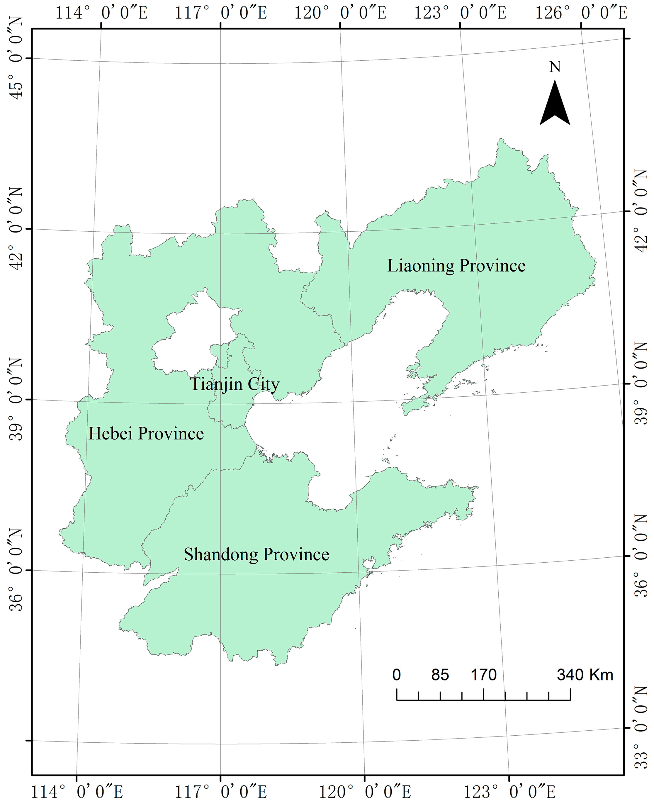
Figure 2.
Methods and processes.

Figure 3.
The coastline changes of provinces, cities, and counties along the Bohai Sea coast ((a) Shandong Province; (b) Hebei Province; (c) Tianjin City; (d) Liaoning Province).
Figure 3.
The coastline changes of provinces, cities, and counties along the Bohai Sea coast ((a) Shandong Province; (b) Hebei Province; (c) Tianjin City; (d) Liaoning Province).

Figure 4.
Shoreline changes in Tanggu District of the Tianjin City ((a) 1985; (b) 2015).

Figure 5.
Shoreline changes in Tanghai County—Fengnan District of the Hebei Province ((a) 1985; (b) 2015).
Figure 5.
Shoreline changes in Tanghai County—Fengnan District of the Hebei Province ((a) 1985; (b) 2015).
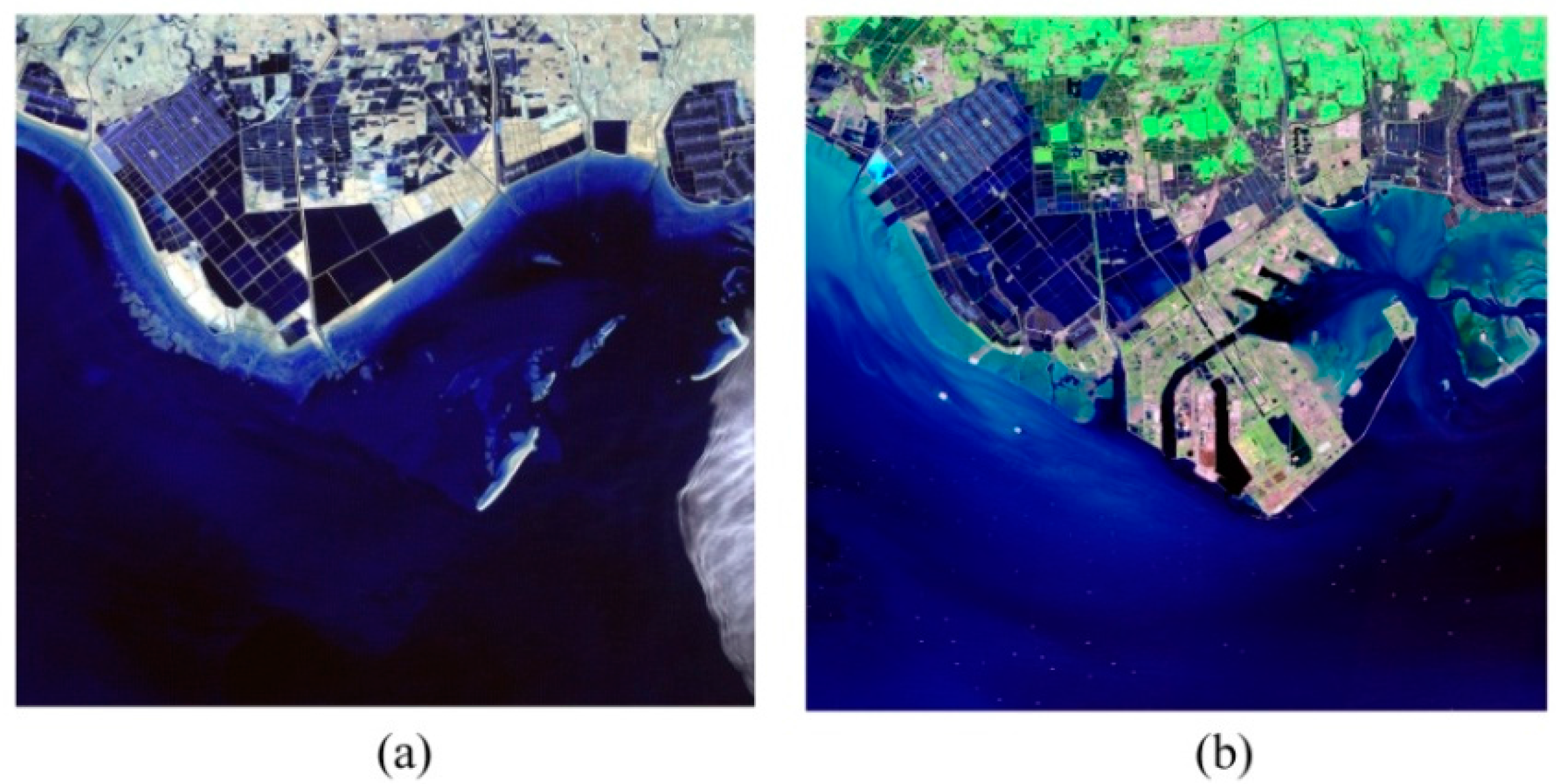
Figure 6.
Shoreline changes in Huanghua City of the Hebei Province ((a) 1985; (b) 2015).


Table 1.
The information of the images used to extract shoreline.
| Year | Number of Images | Path/Row of Images for Each Year | Sensor | Spatial Resolution | Band Used |
|---|---|---|---|---|---|
| 1985 | 7 | 120/32, 120/33, 120/34, 121/32, 121/33, 121/34, 122/33 | TM | 30 m | 5, 4, 3 |
| 1995 | 7 | TM | 30 m | 5, 4, 3 | |
| 2005 | 7 | TM | 30 m | 5, 4, 3 | |
| 2015 | 7 | OLI | 30 m | 5, 6, 4 |
Table 2.
The provincial units and counties adjacent to the Bohai Sea.
| Provincial Units | Counties |
|---|---|
| Shandong Province (a total of 16 counties) | Laishan District, Zhifu District, Fushan District, Penglai City, Longkou City, Zhaoyuan City, Laizhou City, Changyi City, Hanting City, Shouguang City, Guangrao County, Dongying District, Kenli County, Hekou District, Zhanhua County, and Wudi County |
| Hebei Province (a total of 10 counties) | Huanghua City, Fengnan District, Tanghai County, Luannan County, Laoting County, Changli County, Funing County, Beidaihe District, Haigang District, and Shanhaiguan District |
| Tianjin City (a total of 3 districts) | Dagang District, Tanggu District, and Hangu District |
| Liaoning Province (a total of 17 counties) | Suizhong County, Xingcheng City, Longgang District, Lianshan District, Linghai City, Panshan County, Dawa County, Xishi District, Bayuquan District, Gaizhou City, Wafangdian City, Jinzhou District, Ganjingzi District, Xigang District, Lvshunkou District, Shahekou District, and Zhongshan District |
Table 3.
Changes in the coastline and sea area of the Bohai Sea during 1985–2015.
| Year | 1985 | 1995 | 2005 | 2015 |
|---|---|---|---|---|
| Coastline length (km) | 2833.90 | 2878.84 | 3485.68 | 4914.70 |
| Sea area (km2) | 86,639.31 | 86,365.38 | 86,252.15 | 84,525.98 |
| Interval | 1985–1995 | 1995–2005 | 2005–2015 | 1985–2015 |
| Change of length (km) | 44.94 | 606.84 | 1429.02 | 2080.80 |
| Percentage (%) | 1.59 | 21.08 | 41.00 | 73.43 |
| Change of sea area (km2) | −273.93 | −113.23 | −1726.17 | −2113.33 |
| Percentage (%) | −0.32 | −0.13 | −2.00 | −2.44 |
Table 4.
The centroid changes in the sea surface area of the Bohai Sea.
| Year | 1985 | 1995 | 2005 | 2015 |
|---|---|---|---|---|
| Centroid coordinate X (m) | 773,121.34 | 773,168.39 | 773,014.12 | 773,955.49 |
| Centroid coordinate Y (m) | 4,311,894.79 | 4,311,853.50 | 4,311,497.91 | 4,311,111.69 |
| Interval | 1985–1995 | 1995–2005 | 2005–2015 | 1985–2015 |
| Change of displacement (m) | 62.59 | 387.62 | 1017.52 | 1144.14 |
| Change of degrees from north | 131°16′8″ | 197°12′54″ | 112°18′25″ | 133°11′31″ |
Note: The degrees from north considered north to be 0°, and counted in a clockwise direction.
Table 5.
Provincial units and county units with the largest percentage change from 1985 to 2015.
| Interval | 1985–1995 (%) | 1995–2005 (%) | 2005–2015 (%) | 1985–2015 (%) | |||||
|---|---|---|---|---|---|---|---|---|---|
| Provincial Units | Tianjin | 43.65 | Hebei | 61.29 | Tianjin | 122.70 | Tianjin | 273.80 | |
| County units | Shandong | Changyi | 76.28 | Zhanhua | 66.98 | Wudi | 471.95 | Wudi | 310.23 |
| Hebei | Luannan | 52.64 | Tanghai | 325.58 | Fengnan | 149.41 | Huanghua | 329.32 | |
| Tianjin | Dagang | 134.16 | Dagang | −32.20 | Hangu | 200.18 | Tanggu | 297.45 | |
| Liaoning | Linghai | 32.60 | Bayuquan | 49.85 | Gaizhou | 125.71 | Bayuquan | 230.22 | |
Table 6.
The interval distribution of change for counties within each provincial unit.
| Time Interval | Change Percentage | Shandong Province (a Total of 16 Counties) | Hebei Province (a Total of 10 Counties) | Tianjin City (a Total of 3 Districts) | Liaoning Province (a Total of 17 Counties) |
|---|---|---|---|---|---|
| 1985–1995 | <10% | 5 | 4 | 1 | 11 |
| 10–30% | 9 | 2 | 0 | 6 | |
| >30% | 2 | 4 | 2 | 0 | |
| 1995–2005 | <10% | 6 | 2 | 0 | 8 |
| 10–30% | 5 | 3 | 1 | 6 | |
| >30% | 5 | 5 | 2 | 3 | |
| 2005–2015 | <10% | 2 | 0 | 0 | 4 |
| 10–30% | 3 | 5 | 0 | 5 | |
| >30% | 11 | 5 | 3 | 8 | |
| 1985–2015 | <50% | 6 | 2 | 0 | 11 |
| 50–100% | 5 | 4 | 0 | 3 | |
| >100% | 5 | 4 | 3 (all > 200%) | 4 |
Table 7.
Coastline shape indexes for each period 1985, 1995, 2005, and 2015.
| Year | Fractal Dimension (D) | Compact Ratio (C) | Circularity (R) | Square Degree (S) |
|---|---|---|---|---|
| 1985 | 1.07 | 0.35 | 2.89 | 2.56 |
| 1995 | 1.08 | 0.34 | 2.94 | 2.61 |
| 2005 | 1.09 | 0.28 | 3.53 | 3.12 |
| 2015 | 1.12 | 0.20 | 4.95 | 4.39 |
Table 8.
Ideal function model and its corresponding R2.
| Dependent Variable | Independent Variable | Function | Adjusted R2 | Equation |
|---|---|---|---|---|
| L | D | Compound | 0.958 | |
| C | Polynomial | 0.999 | ||
| R | Polynomial | 0.999 | ||
| S | Polynomial | 0.999 | ||
| D (x1) C (x2) | Linear | 0.943 (DW = 1.9) | ||
| A | D | Cubic | 0.984 | |
| C | Polynomial | 0.949 | ||
| R | Cubic | 0.963 | ||
| S | Cubic | 0.964 | ||
| L | Cubic | 0.962 | ||
| D (x1) C (x2) | Linear | 0.962 (DW = 1.9) | ||
| L | Year | Compound | 0.795 | |
| A | Cubic | 0.634 | ||
| D | Compound | 0.877 | ||
| C | Cubic | 0.870 | ||
| R | Compound | 0.794 | ||
| S | Compound | 0.792 |
Note: x denotes the independent variable, and y denotes dependent variable, L denotes the coastline length, and A denotes the sea area in the table. D, C, R, and S denote the fractal dimension, compact ratio, circularity, and square degree successively.
Table 9.
Accuracy rating of the prediction results for coastline length in 2025.
| Prediction Object | Scheme | Prediction Value | C | P | Accuracy Rank |
|---|---|---|---|---|---|
| Coastline length (km) | 1 | 5440.09 | 0.0054 | 1 | good |
| 2 | 5807.92 | 0.0114 | 1 | good | |
| 3 | 6907.49 | 0.1722 | 1 | good | |
| Sea area (km2) | 1 | 84,312.51 | 0.0569 | 1 | good |
| 2 | 83,297.74 | 0.0188 | 1 | good | |
| 3 | 78,414.60 | 0.2794 | 1 | good |
© 2017 by the authors. Licensee MDPI, Basel, Switzerland. This article is an open access article distributed under the terms and conditions of the Creative Commons Attribution (CC BY) license (http://creativecommons.org/licenses/by/4.0/).
Share and Cite
MDPI and ACS Style
Fu, Y.; Guo, Q.; Wu, X.; Fang, H.; Pan, Y. Analysis and Prediction of Changes in Coastline Morphology in the Bohai Sea, China, Using Remote Sensing. Sustainability 2017, 9, 900. https://doi.org/10.3390/su9060900
AMA Style
Fu Y, Guo Q, Wu X, Fang H, Pan Y. Analysis and Prediction of Changes in Coastline Morphology in the Bohai Sea, China, Using Remote Sensing. Sustainability. 2017; 9(6):900. https://doi.org/10.3390/su9060900
Chicago/Turabian StyleFu, Ying, Qiaozhen Guo, Xiaoxu Wu, Hui Fang, and Yingyang Pan. 2017. "Analysis and Prediction of Changes in Coastline Morphology in the Bohai Sea, China, Using Remote Sensing" Sustainability 9, no. 6: 900. https://doi.org/10.3390/su9060900
Note that from the first issue of 2016, this journal uses article numbers instead of page numbers. See further details here.