Uncovering the Driving Factors of Carbon Emissions in an Investment Allocation Model of China’s High-Carbon and Low-Carbon Energy

Abstract

In the view of long-term comprehensive development, the concept of low-carbon economy has long been a concern. In this paper, we build a pure energy-economic system and explore the exact influencing factors in the investment allocation of high-carbon and low-carbon energy with the purpose of mitigating carbon dioxide in the atmosphere. The dynamic analysis shows that the model that we built is applicable for the current market situation and the way we adjust the investments of high-carbon and low-carbon energy are conductive to carbon abatement in the atmosphere. On the basis of the stability analysis and numerical simulation, some strategies are given to decrease the carbon dioxide in the atmosphere. The results show that the social consumption and public consumption behavior are the most important factors responsible for the variation in the atmospheric carbon dioxide. The cleanliness of high carbon presents an obvious mitigating effect on carbon in the atmosphere and the effect of marginal profit of high-carbon energy is the weakest. In addition, enhancing marginal profit, return on investment and investment share of low-carbon energy are beneficial to reduce carbon dioxide in the atmosphere, while a return on investment of high-carbon energy increasing is the detriment of the carbon dioxide in the atmosphere. Finally, we provide carbon mitigation effort by considering both economic development and carbon abatement for policymakers to achieve a desirable emission-reduction effect.

1. Introduction

The global economy has made a great progress with the development of the global industrialization, which cannot be improved without energy. The China Statistical Yearbook shows that China’s total energy consumption was 122,727 million tonnes of coal equivalent (tce) in 1994, but augmenting to 402,138 million tonnes of coal equivalent (tce) in 2013 with an average annual growth rate of over 11%. However, such rapid increase of energy consumption induced the excessive emissions of carbon dioxide, which had intensified the negative effect on environmental quality. In the process of economic development, China is facing great challenges in stimulating low-carbon development. At the Copenhagen conference, China promised to decrease 40–50% of its carbon intensity by 2020 with respect to 2005 levels. This forced the policymakers to consider not only developing the economy but also reducing the atmospheric carbon dioxide. Many researchers have investigated the correlativity between energy consumption, economic growth and carbon emissions.

Large studies have focused on the relationship between the energy consumption and the economic growth in different countries and different time periods [1,2,3,4,5,6,7,8,9,10]. Belloumi [1] held that energy consumption and economic growth had a long-run-bi-directional causal relationship and a short-run unidirectional causality from energy to economic growth. Tsani [4] and Belke et al. [8] also found the existence of bi-directional causal relationship between economic growth and energy consumption. In addition, the research from Lee and Chang [5] and Liddle and Sadorsky [10] showed a bi-directional causal relationship between economic growth and energy consumption. All of these studies have confirmed that there exists a strong relationship between the energy consumption and the economic growth. Furthermore, over 85% of the global energy demand is currently being supported by burning the fossil fuels [11]. Thus, with the further development of the global economy, energy, especially the fossil fuel, will hold an important position in the process of society development for a certain period of time.

On the other hand, the problem of carbon emissions is also a hot topic. The fossil fuel combustion produces large amounts of carbon emissions in the atmosphere and increases the burden of the environment [10]. The Intergovernmental Panel on Climate Change (IPCC) report of 2015 revealed that the 78% of carbon emissions came from the fossil fuels and industrial emissions in the past four decades. Ghali and El-Sakka [9] indicated that the combustion of fossil fuels and industrial production were the primary factors of increasing anthropogenic carbon emissions and these two human activities accounted for 91% of all anthropogenic carbon emissions. In order to facilitate interpretation, we call the fossil fuels (like coal, oil, etc.) high-carbon energy and call renewable energy (as unclear, solar, wind, geothermal, etc.) low-carbon energy [12]. It is worth nothing that, although a tiny share of low-carbon energy, it is increasingly advocated by Chinese government and shows an augmented trend. Globally, the development of low carbon energy will play a significant role in abating carbon emissions because of the near zero-carbon emissions of low-carbon energy sources in the process of energy use and production. Therefore, the use and development of high-carbon energy sources rather than low-carbon affects carbon dioxide in the atmosphere. In addition, part of the anthropogenic carbon dioxide is absorbed by the nature skin in the oceans and on land [13,14,15,16]. In addition, the absorption rate is almost a constant of 57% [17]. That is to say, the main factors affecting the atmospheric carbon dioxide are the combustion of the high-carbon energy in the industrial production, the emissions of social consumption and the absorption of nature.

Faced with global warming and environmental degradation, the effective and feasible approach is to reduce the high-carbon energy consumption and increase the low-carbon energy consumption. It already becomes the common world view and should be a long-term policy for China’s carbon emission reduction targets. IEA World Energy Outlook 2016 estimated that, in the next 25 years, low-carbon energy would be the biggest winner in the race to meet energy demand growth. It was a result of government policy, which was key to a successful energy transition from high-carbon energy to low-carbon energy. Furthermore, Obama [18], president of the United States, confirmed that despite different national policies, low-carbon energy consumption was appropriate and beneficial to all the countries. Many research studies have investigated carbon emissions generated by energy consumption. Wang et al. [19] and Wang and Ye [20] studied the causal relationship between energy consumption, economic growth and carbon emissions. The results showed a unidirectional causal relationship from energy consumption to carbon emissions and economic growth prompted carbon emissions from fossil energy consumption to increase. Xu et al. [21] pointed out that energy structure effect was conductive to promote carbon emissions reduction. Furthermore, policies that promoted a shift to low-carbon energy should be enhanced by government. Li et al. [22] were consistent with that of the results in Xu et al. [21], and this indicated that low-carbon energy growth may lead to an absolute recombination of the China’s energy-economic system. Yang et al. [23] analyzed the means for China to meet the goals in 2020 and predicted that the output of high-carbon and low-carbon energy should be increased by 1.29 times and 74.67% of the 2013 levels by 2020, respectively. Furthermore, technological progress played a critical role in abating carbon emissions. Apart from the above-mentioned methods of reducing carbon emissions, Liu [24] particularly showed that keeping the number of high-carbon industrial firms at a low level did not sustain the security of energy supply. The results also indicated that low-carbon awareness and behavior of firms played a significant role in developing low-carbon energy. In terms of the current raw technology of low-carbon energy, the high-carbon energy will still play an important role in economic growth. Thus, the reduction of high-carbon consumption must be controlled in a reasonable range. Currently, energy structure adjustment is not going to happen overnight, and it is a gradual process that transfers the weight of energy consumption from high-carbon to low-carbon energy.

Of course, many factors can exert significant impacts on energy related carbon emissions, such as investment share, economic level, R&D activities and industrial structure. Meanwhile, a number of research studies have explored the different influential degrees of related factors on carbon emissions. Shao et al. [25] adopted a novel decomposition method to explore dominant factors of carbon emissions changes from China’s mining sector. The results indicated that output scale and carbon intensity were two primary factors of carbon emissions changes, and the energy use effect also played a positive role to carbon emissions mitigation. Zhang et al. [26] found that both the enhancement of efficiency improvement and structural adjustment had substantial abatement potentials for China’s industrial carbon emissions intensity and industrial carbon emissions. In order to achieve China’s 2030 emissions-peak target, efficiency improvement and structural adjustment were necessary and significant. However, the exact measures are relatively difficult to find to directly reflect the economic level and industrial structure. Technological change is also viewed as an crucial factor affecting environmental quality. Shao et al. [27] estimated the degrees of technological changes biased to capital, labor, energy and carbon emissions, indicating that capital and energy efficiency were the two major factors affecting the green technical efficiency. Zhao et al. [28] also thought that economic activity level was a significant factor that affected the decoupling effect of economic growth from carbon emissions in China. In fact, economic growth is closely related to investment [29]. Investment is not only the prerequisite of economic activities but also the main influencing factor of carbon emissions [30]. Furthermore, Shao et al. [31] also had the similar view that investment declined the energy use per unit of output and carbon emissions, improving the environmental quality. However, limited research studies were related to the exact measures for investment allocation of high-carbon and low-carbon energy to decrease energy-related carbon emissions. In this paper, an energy investment dynamic model is built, in which the energy investment allocations are determined by different carbon intensity. On the basis of dynamic characteristics, some main influence factors of the carbon emissions are researched and analyzed, and four strategies are given to decrease the carbon emissions while ensuring the stable economic growth.

2. Establishment of the Model and Its Analysis

In this paper, in order to explore the specific influential factors of carbon abatement, a pure energy-economy system is considered and the influence of other industries is ignored. Firstly, we assume that the economic output is only produced by the energy industry, and that it is mainly used for social consumption and the investment in the energy development. Although many factors affect economic output significantly, this work focuses on capital quantity generated by energy consumption in a pure energy-economic system. Without being against the economic theory, economic output in the pure energy-economic system is expressed as a function of energy consumption. Since the typical dependence on the capital is nearly a constant in the short term, the exact value of capital quantity is a multiple of energy yield.

For the sake of discussion, the influence of the low-carbon energy on the environment is negligible. Meanwhile, the carbon emission (the concomitant of the economic system) is mainly associated with three factors: the combustion of the high-carbon energy, the emissions of social consumption and the absorption by nature. To control the carbon emission level, the decision makers will make an investment distribution between the high-carbon energy and low-carbon energy. A system of energy investment and carbon emission will be built in this section.

2.1. Establishment of the Model

We define the investment shares of the high-carbon energy and the low-carbon energy as $\phi$, $\psi$ respectively, which satisfy the equation $\phi +\psi =1$. In addition, the current carbon emission in the atmosphere at time t is denoted as $x\left(t\right)$. In order to reduce the atmospheric carbon dioxide while developing the economy, a reasonable investment guiding scheme in the energy field should be formulated. In theory, under the situation of larger amounts of carbon emissions in the atmosphere, the policymakers should take measures to mitigate the atmospheric carbon dioxide. The most direct, powerful and effective way is to reduce the supply of high-carbon energy from the supply side. It can be achieved by reducing the investment share of high-carbon energy. That is, the investment share of the high-carbon energy $\phi$ should be a function of $x\left(t\right)$. Similarly, the investment share of the low-carbon energy $\psi$ can be expressed as a function of $x\left(t\right)$.

In our model, we consider a pure energy economy system where the economic output is only determined by the energy factor. That is, the economic output function can be described by two key variables, the low-carbon energy y and the high-carbon energy z. We denote this function as $g(y,z)$. In general, the economic output $g(y,z)$ will be used for social consumption $e$ and energy investment I, i.e.,

$$g(y,z)=e+I.$$

(1)

In the process of energy use and economic development, the combustion of the high-carbon energy and the emissions of social consumption increase the carbon emissions. Meanwhile, the absorption by nature reduces carbon emissions and the absorption rate is almost a constant. For the carbon emission in the atmosphere $x\left(t\right)$, we consider a differential equation as follows:

$$\dot{x}\left(t\right)=f(z\left(t\right),e,x\left(t\right)),$$

(2)

where the partial derivatives $\frac{\partial f}{\partial \mathrm{z}}$ (the carbon coefficients of the high-carbon energy) and $\frac{\partial f}{\partial e}$ (the carbon coefficients of the social consumption) are positive, and the partial derivative $\frac{\partial f}{\partial x}$ (the absorption rate of nature) is almost a negative constant.

The low-carbon energy output $y\left(t\right)$ and high-carbon energy output $z\left(t\right)$ are the function of energy investment I. Currently, low-carbon energy use is increasingly supported by the Chinese government and experiences an increasing trend. The proportion of low-carbon energy in China’s total energy consumption is 6.3% in 1993, while increasing to 14.5% in 2015. However, compared with the high proportion of high-carbon energy, the low-carbon energy occupies a tiny share in total energy consumption. In the premise of no large-scale investment project of high-carbon energy, China’s current technology level of high-carbon energy is relatively mature. However, the low-carbon energy development requires huge capital accumulation. We assume the technology of high-carbon energy is relatively mature at time k and k is a constant. To simplify the mathematical analysis, we will suppose that the low-carbon energy output $y\left(t\right)$ is determined by the total input ${\int }_k^t{I}_1\left(s\right)ds$, and the output of the high-carbon energy $z\left(t\right)$ is determined by its investment at time t. Economic output of low-carbon energy is a result of capital accumulation. The specific equations are as follows:

$$y\left(t\right)=f_1({\int }_k^t{I}_1\left(s\right)ds),$$

(3)

$$z\left(t\right)=f_2\left(I_2\left(t\right)\right),$$

(4)

where $I_1$ is the investment of low-carbon energy and $I_2$ is the investment of high-carbon energy, $f_1$ is the productive function of low-carbon energy and $f_2$ is the productive function of high-carbon energy.

Note that $\psi$ and $\phi$ are used to describe the investment shares of the low-carbon energy and the high-carbon energy. We then have

$$I_1\left(t\right)=I\left(t\right)\psi \left(x\left(t\right)\right),I_2\left(t\right)=I\left(t\right)\phi \left(x\left(t\right)\right).$$

(5)

Taking Equation (2) into Equation (5), we obtain

$$I_1\left(t\right)=\left[g\left(y\right(t),z(t\left)\right)-e\right]\psi \left(x\left(t\right)\right),I_2\left(t\right)=\left[g\left(y\right(t),z(t\left)\right)-e\right]\phi \left(x\left(t\right)\right).$$

(6)

Substituting Equation (6) into Equations (3) and (4), we get

$$y\left(t\right)=f_1({\int }_k^t\left[g\left(y\right(s),z(s\left)\right)-e,\right]\psi \left(x\left(s\right)\right)ds)$$

(7)

$$z\left(t\right)=f_2\left(\left[g\right(y\left(t\right),z\left(t\right))-e]\phi \left(x\right(t\left)\right).\right)$$

(8)

To sum up, we obtain the equations as the following:

$$\left\{\begin{array}{c}\dot{x}\left(t\right)=f(x\left(t\right),e,z\left(t\right)),\hfill \\ y\left(t\right)=f_1{\int }_k^t\left[g\left(y\right(s),z(s\left)\right)-e\right]\psi \left(x\left(s\right)\right)ds,\hfill \\ z\left(t\right)=f_2\left(\left[g\right(y\left(t\right),z\left(t\right))-e]\phi \left(x\right(t\left)\right)\right).\hfill \end{array}\right.$$

(9)

2.2. Parameters of the Model

In order to analyze conveniently, the functions $f,g,f_1,f_2$ and parameters $\phi ,\psi$ will be defined. Simply, the carbon coefficients of the high-carbon energy $\frac{\partial f}{\partial z}$, the carbon coefficient of the social consumption $\frac{\partial f}{\partial e}$ and the absorption rate of nature $\frac{\partial f}{\partial x}$ are denoted as l,$\mu$, $-m$, respectively. The function $f\left(x\right(t),e,z(t\left)\right)$ can be written as:

$$f\left(x\right(t),e,z(t\left)\right)=lz\left(t\right)+\mu e-mx\left(t\right).$$

(10)

Thereinto, l is related to the cleanliness of the high-carbon energy, $\mu$ reflects the spending habits of the public, and the absorption rate of nature $-m$ is always a constant.

As the increase of $x\left(t\right)$ would cause the $\phi$ mitigation, the function $\phi \left(x\right)$ is infinitely close to zero when $x\left(t\right)$ is enormous enough, i.e., $\frac{d\phi }{dx}<0$ and $\underset{x\to +\infty }{lim}\phi \left(x\right)=0$. Since the sum of high-carbon energy investment coefficient $\phi$ and low-carbon energy investment coefficient $\psi$ is 1, we get $\frac{d\phi }{dx}+\frac{d\psi }{dx}=0$. The investment share function $\psi \left(x\right)$ for low-carbon energy must satisfy $\frac{d\psi }{dx}>0$. In conclusion, the high-carbon investment share function $\phi \left(x\right)$ and low-carbon investment share function $\psi \left(x\right)$ satisfy the following conditions:

$$\left\{\begin{array}{c}\phi +\psi =1,\hfill \\ \frac{d\phi }{dx}<0,\hfill \\ \frac{d\psi }{dx}>0,\hfill \\ \underset{x\to +\infty }{lim}\phi \left(x\right)=0.\hfill \end{array}\right.$$

(11)

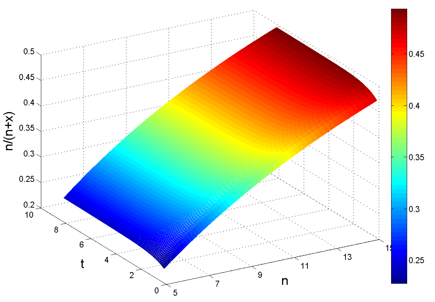
Simultaneously, the investment coefficients of the high-carbon energy $\phi \left(x\right(t\left)\right)$ and the low-carbon energy $\psi \left(x\right(t\left)\right)$ satisfying the first formula in Equation (11) are chosen as

$$\left\{\begin{array}{c}\phi \left(x\left(t\right)\right)=\frac{1}{1+\frac{x\left(t\right)}{n}},\hfill \\ \psi \left(x\left(t\right)\right)=\frac{1}{1+\frac{n}{x\left(t\right)}},\hfill \end{array}\right.$$

(12)

where n follows from some government decision. When a number of carbon emissions exist in the atmosphere, adjusting n at a low level decreases the investment share of high-carbon energy and boosts investment share of low-carbon energy, which is conductive to carbon reduction.

For convenience, $g,f_1$ and $f_2$ are chosen as linear functions. In the pure energy-economic system, the specific form of economic presents in Equation (13), aiming to explore the correlation between energy consumption and economic output. Of course, nonlinear function is far better to describe the exact relationship between these two variables and get the more precise numerical solutions. However, in fact, the mutual relationships among the main variables would not be influenced regardless of linear or nonlinear function relationship. Thus, we simply express g as follows:

$$g(y\left(t\right),z\left(t\right))=m(a_{1}z\left(t\right)+b_{1}y\left(t\right))=az\left(t\right)+by\left(t\right),$$

(13)

$$f_1({\int }_k^t{I}_1\left(s\right)ds)=d{\int }_k^t{I}_1\left(s\right)ds,f_2\left(I_2\left(t\right)\right)=c{I}_2\left(t\right),$$

(14)

So

$$f_1({\int }_k^t{I}_1\left(s\right)ds)=d{\int }_k^t{I}_1\left(s\right)ds={\int }_k^{t}d\left(az\right(s)+by(s)-e)\psi \left(x\right(s\left)\right)ds,$$

(15)

$$f_2\left(I_2\left(t\right)\right)=c{I}_2\left(t\right)=c(az\left(t\right)+by\left(t\right)-e)\phi \left(x\left(t\right)\right),$$

(16)

where coefficients $a_1,b_1$ denote the marginal profits of high-carbon and low-carbon energy; m is a constant that represents the reciprocal of dependency of energy output on economic output in the system; and $c,d$ are the returns on investment of the high-carbon and low-carbon energy. Furthermore, the returns on investment of the high-carbon and low-carbon energy are related to the production technical level of the high-carbon and low-carbon energy, respectively.

Taking Equations (10), (12), (15) and (16) into Equation (9), we obtain

$$\left\{\begin{array}{c}\dot{x}\left(t\right)=lz\left(t\right)+\mu e-mx\left(t\right),\hfill \\ y\left(t\right)=d{\int }_k^t(az\left(s\right)+by\left(s\right)-e)\frac{1}{1+\frac{n}{x\left(t\right)}}ds,\hfill \\ z\left(t\right)=c(az\left(t\right)+by\left(t\right)-e)\frac{1}{1+\frac{x\left(t\right)}{n}}.\hfill \end{array}\right.$$

(17)

Equation (17) can be rewritten as

$$\left\{\begin{array}{c}\dot{x}\left(t\right)=lc(by\left(t\right)-e)\frac{n}{n+x\left(t\right)-can}+\mu e-mx\left(t\right),\hfill \\ \dot{y}\left(t\right)=d(by\left(t\right)-e)\frac{x\left(t\right)}{n+x\left(t\right)-can}.\hfill \end{array}\right.$$

(18)

The change of parameters $a,b,c,d,e,n,l,\mu$ would affect the output of high-carbon and low-carbon energy and the carbon emissions. These parameters would also influence the convergence rate of system.

2.3. Equilibrium and Stability of the System

Proposition 1.

(Equilibrium point) If the unit marginal contribution of low-carbon energy is positive, Equation (18) admits an effective equilibrium point: $(\frac{e\mu }{m},\frac{e}{b})$.

Proof. 

The equilibrium point can be given by the following Equation:

$$\left\{\begin{array}{c}lc(by-e)\frac{n}{n+x-can}+\mu e-mx=0,\hfill \\ d(by-e)\frac{x}{n+x-can}=0.\hfill \end{array}\right.$$

(19)

Then, the equilibrium points of the system can be obtained as $(\frac{e\mu }{m},\frac{e}{b})$, $(0,\frac{e}{b}+\frac{e\mu (ca-1)}{blc})$.

Note that $x,y$ and z must be any non-negative values. However, at the point of $(0,\frac{e}{b}+\frac{e\mu (ca-1)}{blc})$, the output of high-carbon energy $z$ will be asymptotically stable at the negative value $-\frac{e\mu }{l}$. Meanwhile, at the point of $(\frac{e\mu }{m},\frac{e}{b})$, z will be asymptotically stable at zero. Thus, the equilibrium point of $(0,\frac{e}{b}+\frac{e\mu (ca-1)}{blc})$ should be invalid. Equation (18) admits only one effective equilibrium point $(\frac{e\mu }{m},\frac{e}{b})$ in the phase space. ☐

Proposition 1 indicates that the equilibrium state of carbon dioxide depends on the product of social consumption and the consumption habits of the public. The smaller social consumption or the better consumption habits of the public benefit carbon emissions mitigation.

Meanwhile, the equilibrium state of pure economic output equal to $az+by=b·\frac{e}{b}=e$, which depends on the social consumption. Thus, the value of e should not be too small to guarantee the economic growth. It is an ideal state.

Therefore, in a short time, to realize the economic energy, the adjustment of the social consumption is an effective choice. In the long run, the best way to reduce the carbon emissions and steady economic growth is to form better consumption spending habits of the public.

Proposition 2.

If $\frac{e}{m}<\frac{can-n}{\mu }$ , system (18) is asymptotically stable and the equilibrium point $(\frac{e\mu }{m},\frac{e}{b})$ is positive.

Proof. 

The Jacobi matrix at the point of $(\frac{e\mu }{m},\frac{e}{b})$ is

$$\left[\begin{array}{cc}-m\hfill & \frac{lcb}{n+\frac{e\mu }{m}-can}\hfill \\ 0\hfill & \frac{bd\frac{e\mu }{m}}{n+\frac{e\mu }{m}-can}\hfill \end{array}\right].$$

The eigenvalues of the Jacobi matrix are ${\lambda }_1=\frac{bd\frac{e\mu }{m}}{n+\frac{e\mu }{m}-can}$, ${\lambda }_2=-m$.

Corresponding to the Routh–Hurwitz criterion, all of the eigenvalues of Equation (18) are negative under the following conditions: $\frac{e}{m}<\frac{can-n}{\mu }$. In this case, the equilibrium point $(\frac{e\mu }{m},\frac{e}{b})$ will be asymptotically stable. ☐

Furthermore, the condition $\frac{e}{m}<\frac{can-n}{\mu }$ can be changed as $n>\frac{e\mu }{(ca-1)m}$. Then, the investment share of the high-carbon energy is $\phi \left(x\right)=\frac{n}{n+x}>\frac{1}{1+\frac{x(ca-1)m}{e\mu }}$, which is positive to the social consumption and the consumption habits of the public, and negative to the values of the carbon emissions, the marginal contribution of high-carbon energy, the productive technology level of the high-carbon energy. That is, the investment of high-carbon energy can be reduced properly with the decrease of social consumption or the better consumption habits if the unit marginal contribution of high-carbon energy and the productive technology level of the high-carbon energy are almost invariant.

The in-equation $\frac{e}{m}<\frac{can-n}{\mu }$ also can be written as $e<\frac{(ca-1)mn}{\mu }$. It means that the maximal consumption must be less than the value $\frac{(ca-1)mn}{\mu }$. In the condition of better spending habits, the maximal social consumption can be raised when the investment coefficient, the productive technology level of the high-carbon energy and the unit marginal contribution of high-carbon energy are confirmed.

Therefore, decision makers should fully consider the consumption habits of the public currently, investment allocation and the distribution of social economic output.

2.4. Numerical Simulations

In this section, all of the parameters should satisfy the above inequality $e<\frac{(ca-1)mn}{\mu }$. The evolution of low-carbon energy output and carbon emissions for different initial values are simulated in Figure 1 and Figure 2 firstly. Then, the evolution of carbon emissions are analyzed while one of the parameters $a,b,c,d,e,n,l,\mu$ changes with time (Figure 3, Figure 4, Figure 5, Figure 6, Figure 7, Figure 8, Figure 9, Figure 10 and Figure 11). In the long run, the time to realize the low-carbon economy can be observed in Figure 12, Figure 13, Figure 14 and Figure 15. In the following simulations, the parameter $m$ is normalized and defined to $m=1$.

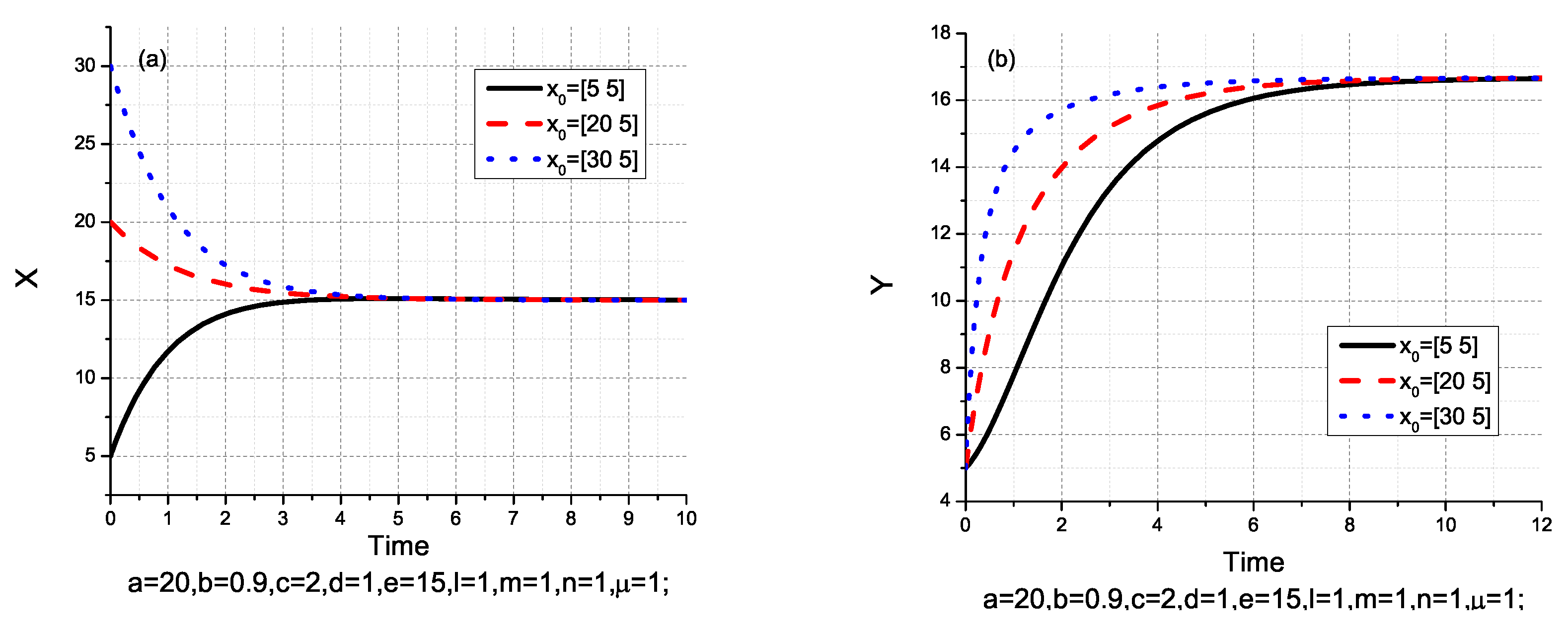
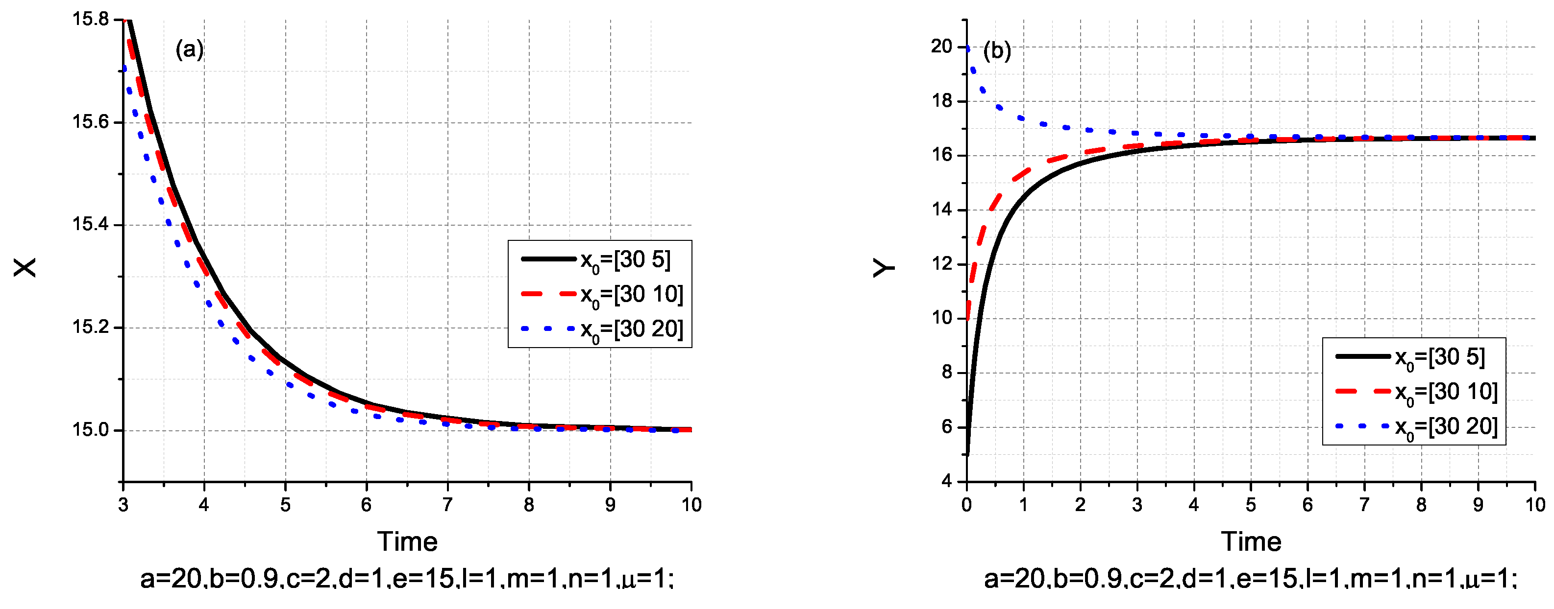
The evolution of carbon emissions x and low-carbon energy y with the initial conditions as (5, 5), (20, 5) and (30, 5) are shown in Figure 1, and with the initial conditions as (30, 5), (30, 10) and (30, 25) are shown in Figure 2.

Figure 1 and Figure 2 indicate that the initial values affect the change trend and the convergence speed of the low-carbon output and the carbon emissions. If the initial value of carbon emissions is larger, the investment allocation scheme we use will reduce carbon emissions. If the initial value of low-carbon energy output is too small, the time that carbon emissions increases up to balance will be relatively long. It is worth nothing that the initial levels of low-carbon energy have no significant effect on evolution trend of carbon in atmosphere. Namely, the initial low-carbon level does not affect carbon dioxide in atmosphere.

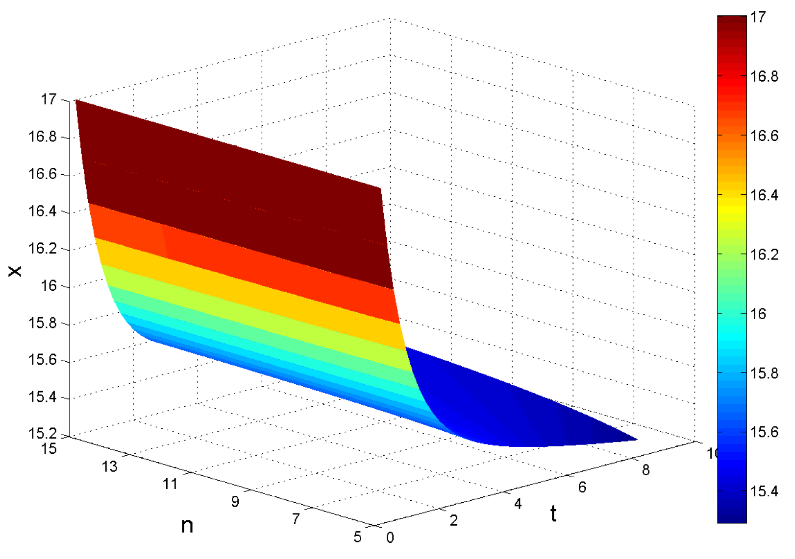
Apart from the impact of initial values, the evolution processes of atmospheric carbon dioxide, while one of the parameters $a,b,c,d,e,n,l,\mu$ changes with time, are presented in Figure 3, Figure 4, Figure 5, Figure 6, Figure 7, Figure 8, Figure 9, Figure 10 and Figure 11.

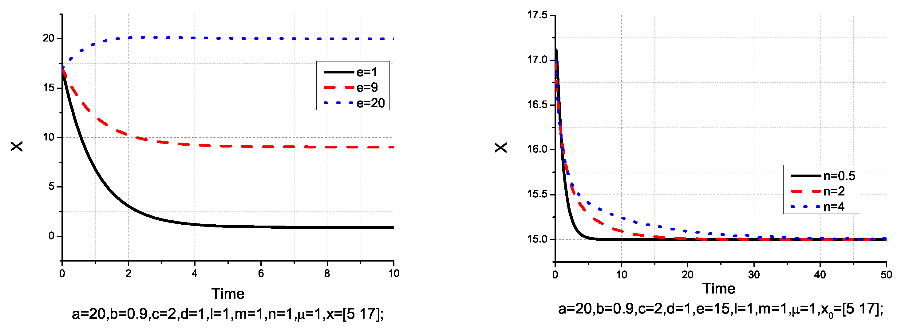
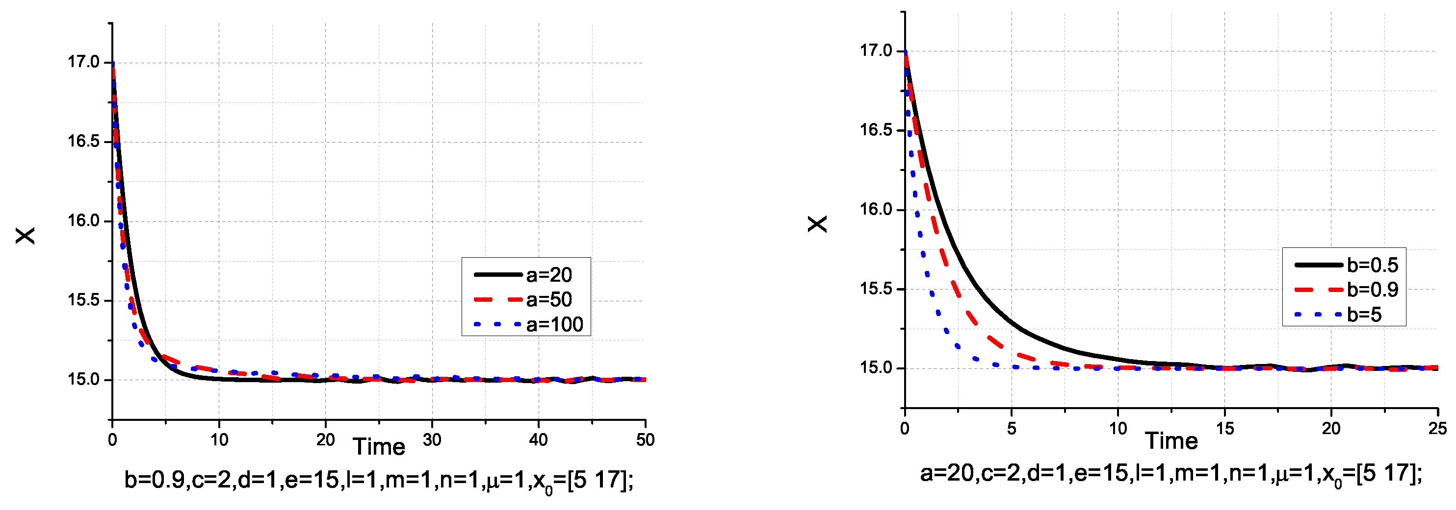
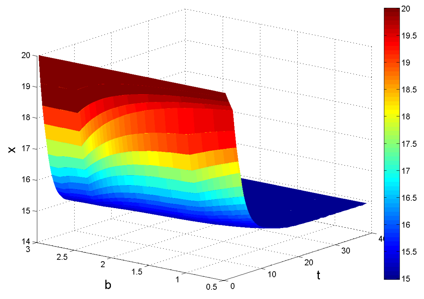
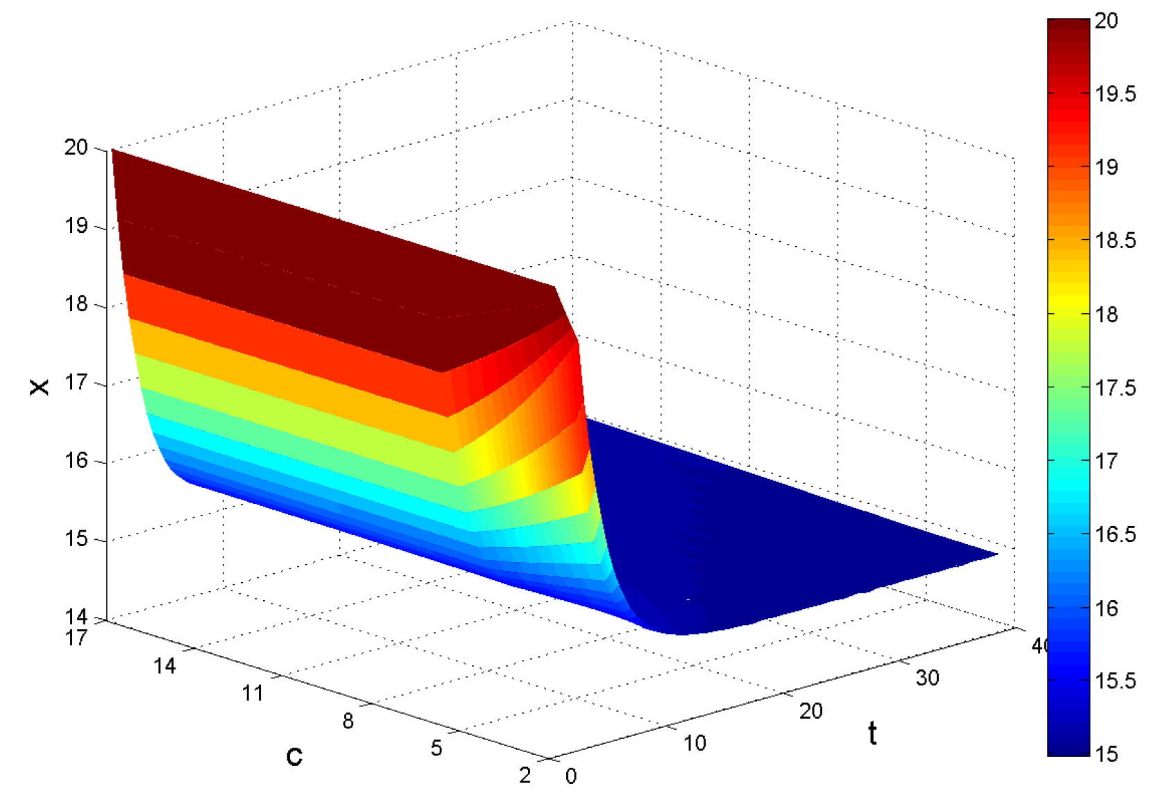
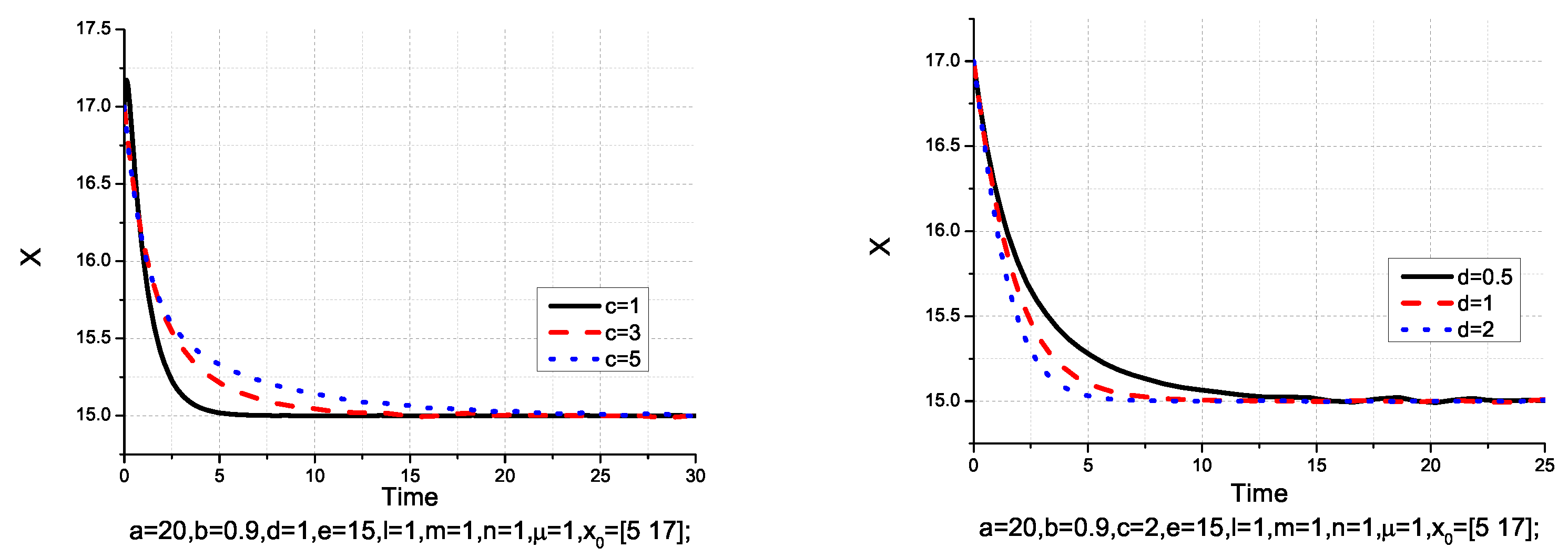
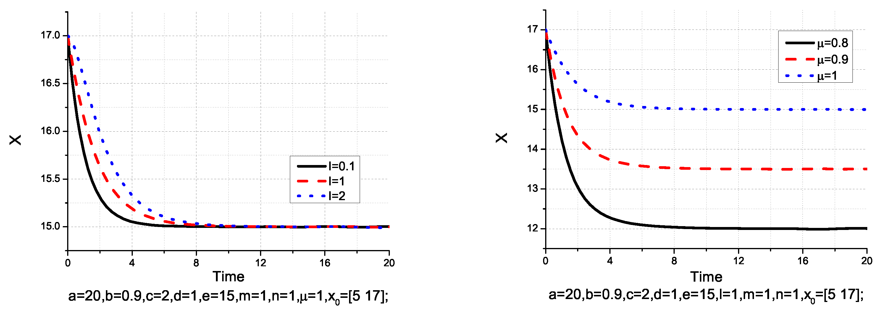
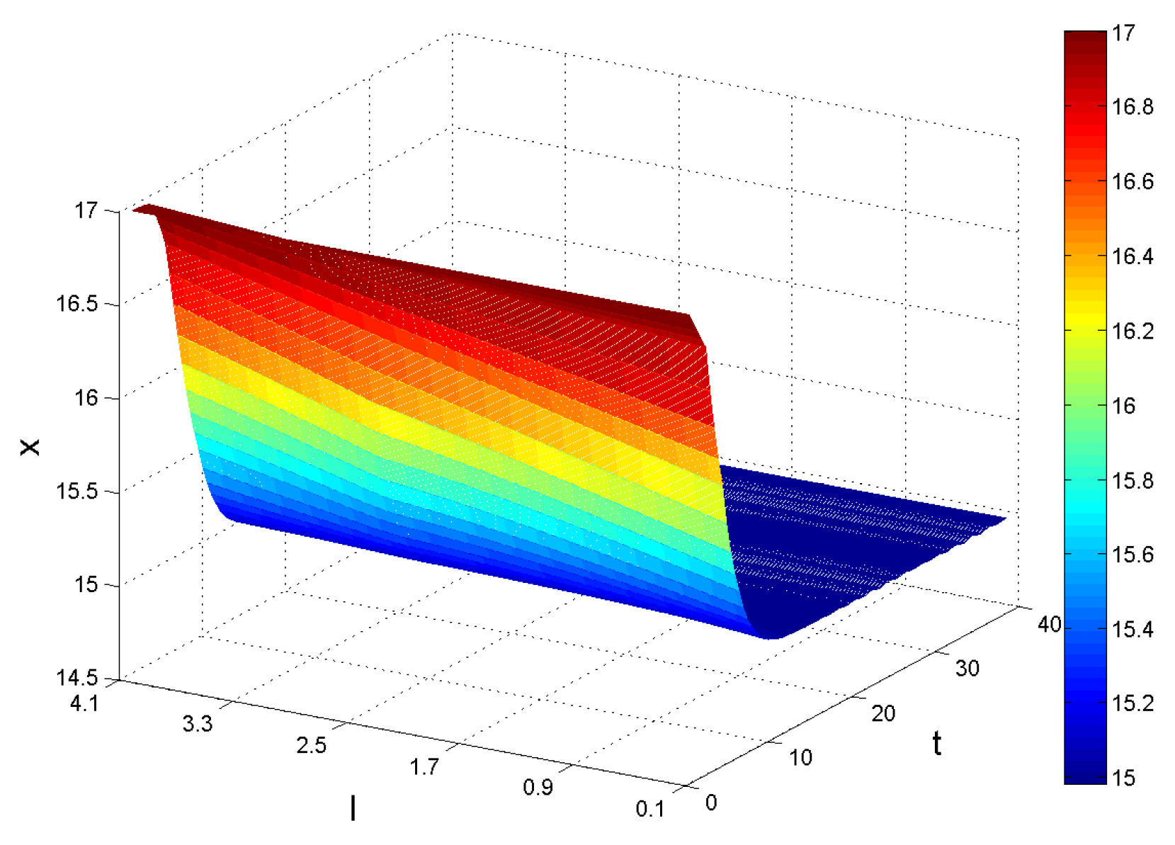
It is clear that there is a similar trend for each factor apart from the factor n, though their detailed values are different. Overall, the parameters $a,b,c,d,e,n,l,\mu$ affect atmospheric carbon dioxide. Figure 3, Figure 4, Figure 5 and Figure 6 show that there exists a minim carbon emission when one of $a,b,c,d$ changes in a short time. Figure 7, Figure 8 and Figure 9 indicate that the carbon emission will be increased when the parameter l, $\mu$ or e enlarges in a short time.

From Figure 10 and Figure 11, we get that n and $\frac{n}{n+x}$ have the same changed tendency, and the carbon emissions will be increased with the parameter n (or $\frac{n}{n+x})$ enlargement in a short time.

In order to analyze the change of carbon emissions over a long time, we discuss differences of contributions of various factors to carbon dioxide in the atmosphere. Unlike the analysis in Figure 4, Figure 5, Figure 6, Figure 7, Figure 8, Figure 9, Figure 10 and Figure 11, the specific influential directions of parameters at some stages are shown in Figure 12, Figure 13, Figure 14 and Figure 15. 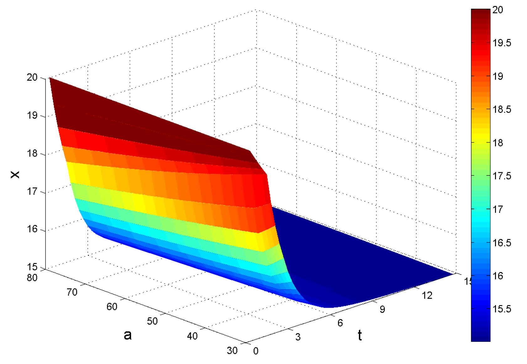Specifically, Figure 12 presents the influence of marginal profit of high-carbon and low-carbon energy on carbon in the atmosphere, respectively. 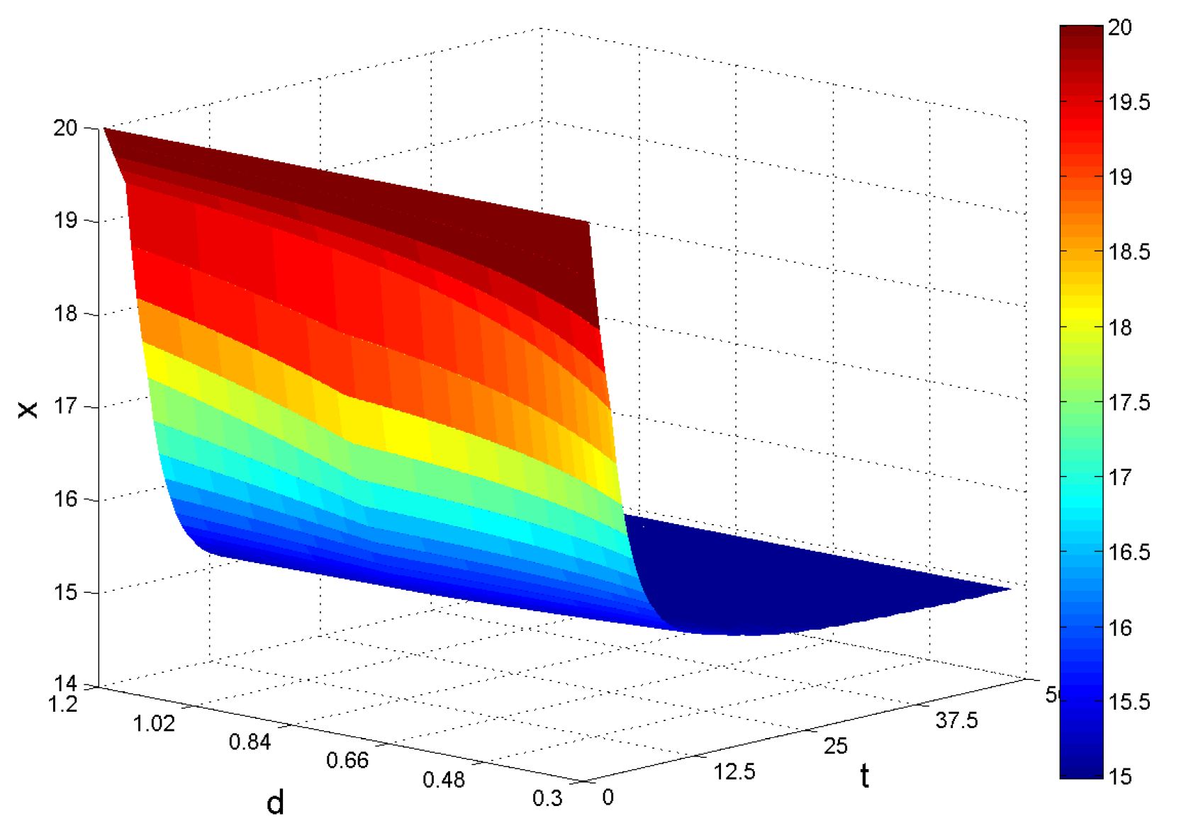Figure 13 describes the evolution of carbon with the change of the value of return on investment. 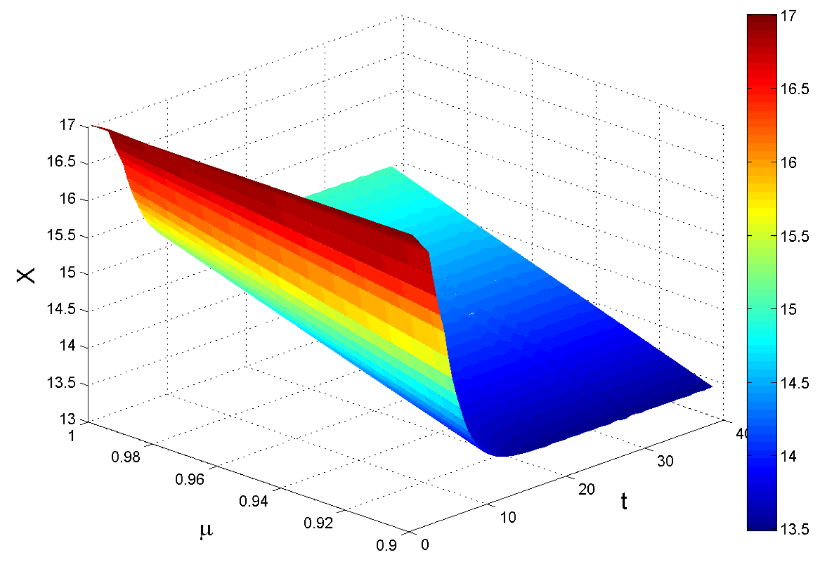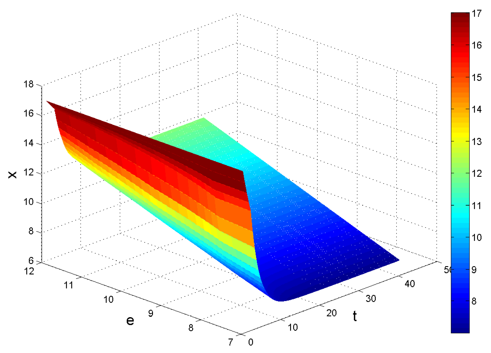The carbon coefficient of high-carbon energy and social consumption as influence parameters are analyzed in Figure 14. In the end, the impact of social consumption level and government adjustment on carbon dioxide in the atmosphere are depicted in Figure 15.

It is clear that the trend of $\mu$ (consuming behavior of social) and e (social consumption) present an obvious effect on carbon dioxide in atmosphere, indicating the dominant role of social behavior in boosting carbon abatement, while a (the marginal profit of high-carbon energy) remains a tiny effect on carbon dioxide in the atmosphere. With respect to the influencing factors $c,l,n$, although their fluctuation are less than $\mu ,e$, they have highly coincident trends. When increasing the values of $c,l,n$, carbon dioxide in the atmosphere mitigates with time at different change rates. Furthermore, l (carbon coefficient of high-carbon energy) falls at the fastest rate compared with the decline rate of $c,n$. Hence, from the perspective of time achieving the balance state, there is no obvious difference between the variable trend of c (the return on investment of high-carbon energy) and n (the government regulation). On the contrary, b (the marginal profit of low-carbon energy) and d (the return on investment of low-carbon energy) show the reverse variation trends compared with $c,n$. In general, the time of carbon dioxide in the atmosphere getting close to the stable state will become shorter when the decrease of $a,c,l,n$ and the increase of $b,d,e$. Furthermore, the value of parameter $\mu$ and e impact the emissions of carbon significantly. Furthermore, the smaller $\mu$ and e will have smaller carbon emissions.

3. Conclusions

In this paper, we focus on carbon mitigation in an investment allocation model of high-carbon and low-carbon energy. The simulation analysis based on a novel model to explore the determinants of the changes of carbon dioxide in the atmosphere, including energy-related and social consumption-related carbon emissions. In order to highlight the significant role of investment in atmospheric carbon dioxide, we introduce the investment share and return on investment in the model. The mathematical analysis and simulation show that parameters $a,b$ (the marginal profits of high-carbon and low-carbon energy), $c,d$ (the returns on investment of high-carbon and low-carbon energy), l (the carbon coefficient of high-carbon energy), $\mu$ (the carbon coefficient of social consumption), e (the social consumption) and n (the government regulation) have significant influence on the volatility of the carbon in the atmosphere to some extent.

The results suggest that the social consumption and consumption behavior play a significant role in influencing carbon dioxide in the atmosphere. Changes in lifestyles and consumer behaviors are not only the main contributors to ameliorate the carbon in the atmosphere but also accord with the concept of low-carbon consumption, which is vigorously promoted by Chinese government. In addition, the atmospheric carbon dioxide is tightly bound to the carbon coefficient of high-carbon energy, which is closely related to the cleanliness of high-carbon energy. Thus, technical progress in improving the cleanliness of high-carbon energy is central to carbon mitigation. It is noteworthy that the marginal profit, return on investment and investment ratio have joint contribution to abate carbon dioxide in the atmosphere. Overall, there is a great possibility for abating emissions by adjusting these influential factors. The aim can be achieved through the realization of some means and policies.

Firstly, low-carbon restructuring of energy consumption structure should be the focus of policy formulation because of its crucial role in carbon mitigation. Shifting to low-carbon consumption and abating high-carbon energy consumption is always regarded as a feasible and effective approach to shift the model of economic development and realize the low-carbon development. Although it is more difficult to adjust energy structure than any other factors because of the energy consumption structure dominated by coal in China for a long time, resulting in a tiny share of low-carbon energy, it can bring a significant benefit in the long term. Furthermore, the consumer awareness and behavior have a significant effect on the atmospheric carbon dioxide. Thus, the government should adjust investment structure and advocate low-carbon consumption throughout society.

Secondly, simulating technological innovation is an effective way to mitigate carbon dioxide in the atmosphere. Based on the above results, the cleanliness of high-carbon energy, marginal profit and return on investment of low-carbon affect the carbon abatement significantly and these influential factors all have direct connection with technical improvement. Even so, many enterprises do not put the technical innovations at a critical position due to the enormous cost and smaller possible income. Thus, a series of effective stimulating measures of technical innovation and adoption must be considered into the policy formulation.

Finally, policymakers should seek a trade-off between economic development and emissions reduction. Although the central role of low-carbon energy in abating carbon in the atmosphere, the importance of high-carbon energy should not be neglected. In terms of the current development level of low-carbon energy, if the investment adjustment is partial to low-carbon energy excessively, it may induce the energy dilemma and social insecurity caused by energy shortage. Thus, on the one hand, enhancing the proportion of low-carbon energy plays a critical in carbon reduction, on the other hand, under the premise of economic development, controlling the consumption of high-carbon energy will be a benefit to carbon abatement.