3.1. Soil Water Dynamics and Irrigation
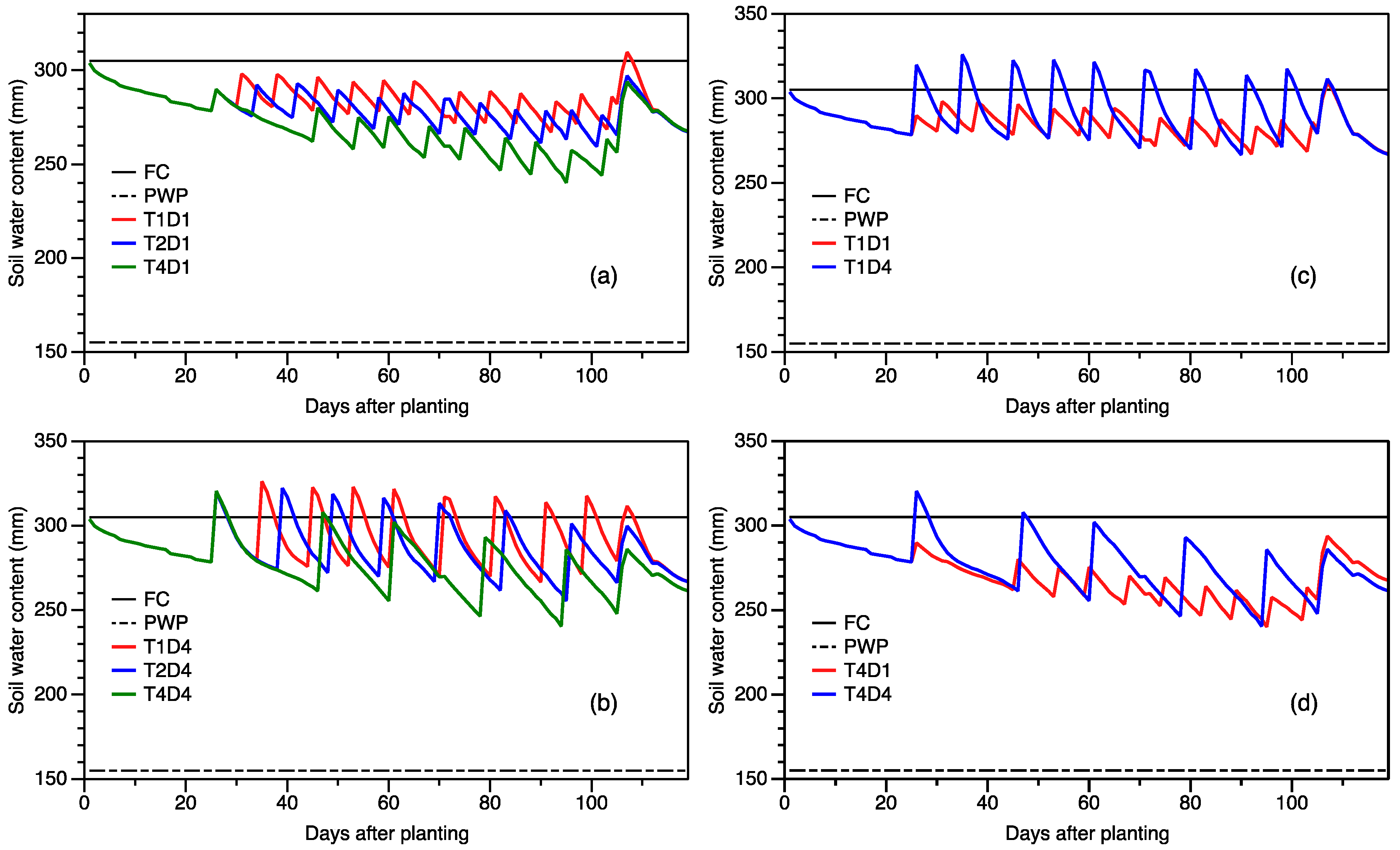
Figure 1 illustrates the simulated seasonal variation of soil water content in the 1-m soil profile depth for the normal characteristic season for selected strategies. In general, as the depletion levels increased, the frequency of water application decreased, since the irrigation was triggered later (
Figure 1a,b). Additionally, it can be observed (
Figure 1c,d) that the lower the application depth (for the same depletion level), the greater the frequency of water application. These observations have important implications, as crop productivity depends not only on the timing and severity of water deficits, but is also influenced by the duration of the drying cycle between water application [
7,
14,
25]. Comparison between the presented strategies shows that in general, soil moisture deficits were also more pronounced at high depletion levels (
Figure 1a), especially at a low water depth (
Figure 1d). Similar observations were made for the dry and wet characteristic seasons, as this irrigation scheduling approach was based on the percent depletion of water in the root zone.
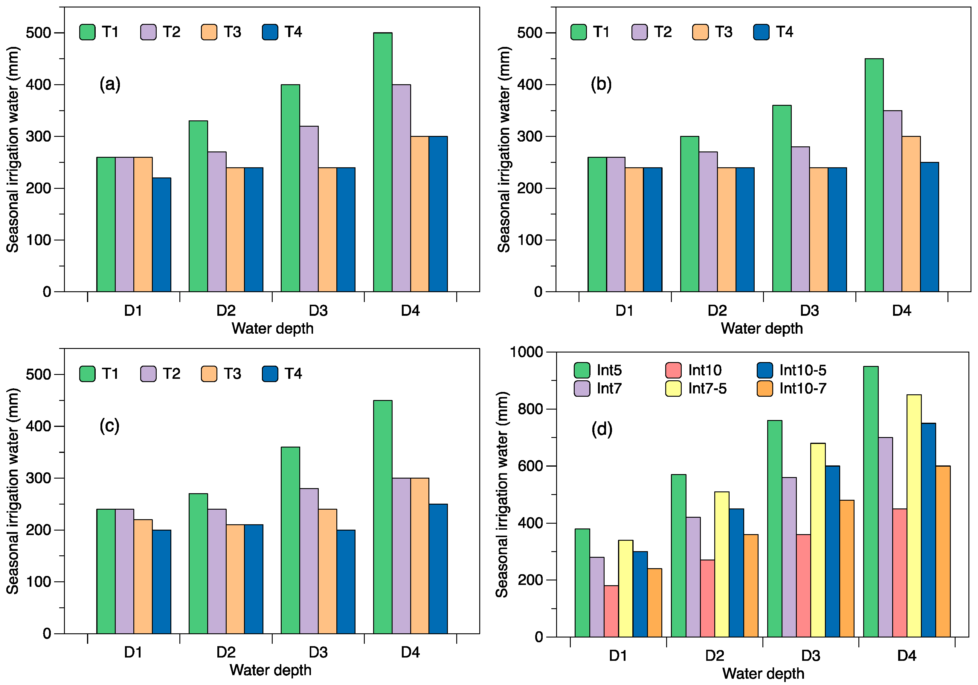
Simulated seasonal water applied for the various depletion levels at varying water application depths is depicted in
Figure 2a–c for the three characteristic seasons. The results presented show that for a dry season, the seasonal water applied varied from 260 to 500 mm, 260 to 400 mm, 260 to 300 mm and 220 to 300 mm for depletions levels 30% (T1), 40% (T2), 50% (T3) and 60% (T4), respectively, depending on water application depth. Similarly, for a characteristic normal season, the respective ranges for these depletion levels were 260–450 mm, 260–350 mm, 240–300 mm and 240–250 mm. The quantities simulated for the characteristic wet season were smaller with T1, T2, T3 and T4 having ranges of 240–450 mm, 240–300 mm, 220–300mm and 200–250 mm, respectively. The ANOVA test indicated highly significant differences (
p < 0.01) in seasonal water applied among the five schedules, which can be attributed to the frequencies of irrigation. In general, a typical range of crop water requirement for maize crop is about 500–800 mm [
14]. The simulated irrigation water supplied under the interval irrigation management is depicted in
Figure 2d. As this management is based on water application at predefined intervals, the same amount of water was supplied for all characteristic seasons. The simulated water applied varied from a low of 180 mm in Int10D1 to a high of 950 mm in Int5D4. The variable interval schedules (Int7–5, Int10–5 and Int10–7) where the intervals between irrigation applications during the reproductive growth stage were reduced recorded higher water application amounts than their fixed counterparts (Int7, Int10).
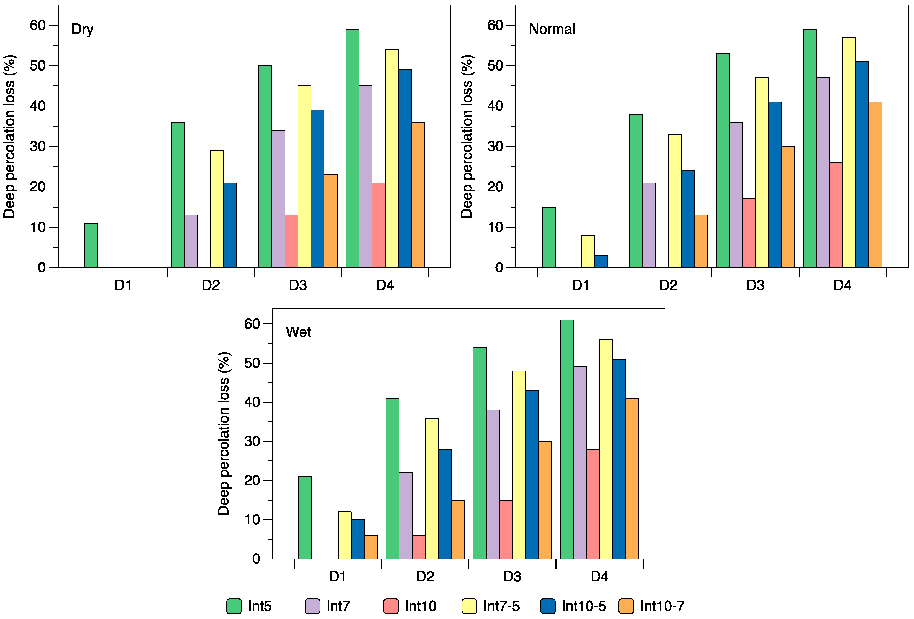
Deep percolation loss was considerably higher for the interval scheduling method than the depletion method. For the depletion scheduling method, losses were observed for only a few combinations generally occurring for the larger water depths. The most significant losses observed for the dry and normal season were 9%, 22% and 11% and 11%, 22% and 12%, respectively, for the respective strategies T1D3, T1D4 and T2D4, and for the wet season, slightly higher amounts of 11%, 24%, 8% and 13% were simulated for T1D3, T1D4, T2D3 and T2D4, respectively. These values are presented as a percentage of the total water applied (irrigation + rainfall). The deep percolations simulated in AquaCrop for the various interval schedules at various water application depths are depicted in
Figure 3. As can be observed, losses increased with an increase in water application depth per irrigation, and values were higher in the characteristic wet season. Across the three characteristic seasons, the deep percolation losses for Int5, Int7, Int10, Int7–5, Int10–5 and Int10–7 varied between 11% and 61%, 0% and 49%, 0% and 28%, 0% and 57%, 0% and 51% and 0% and 41% of the total water applied, respectively. In terms of water application depths, an application of 40 and 50 mm often resulted in high loss of water to deep percolation; five out of the 36 cases resulted in losses less than 21%; and most (four) of these cases occurred for the schedule Int10. Considering the daily intervals, across the three characteristic seasons, the more frequent five-day schedule (Int5) continually recorded the greatest percolation losses for any water depth (
Figure 3) with nine out of the 12 cases resulting in losses greater than 36%. Overall, the 10-day schedule (Int10) followed by the 10-day-7-day schedule (Int10–7) produced the lowest losses and greater number of 0% loss. High deep percolation loss (up to 1133 mm) at short irrigation intervals and high water application have been reported in other simulation studies evaluating interval scheduling [
12,
14]. Besides the obvious negative impact on the efficiency of agricultural water use, Igbadun and Salim [
14] highlight that some of the consequences of high percolation losses include rapid build-up of the water table, the increase in soil salinity and water logging, which leads to poor yield due to low soil temperatures and poor aeration of plant roots.
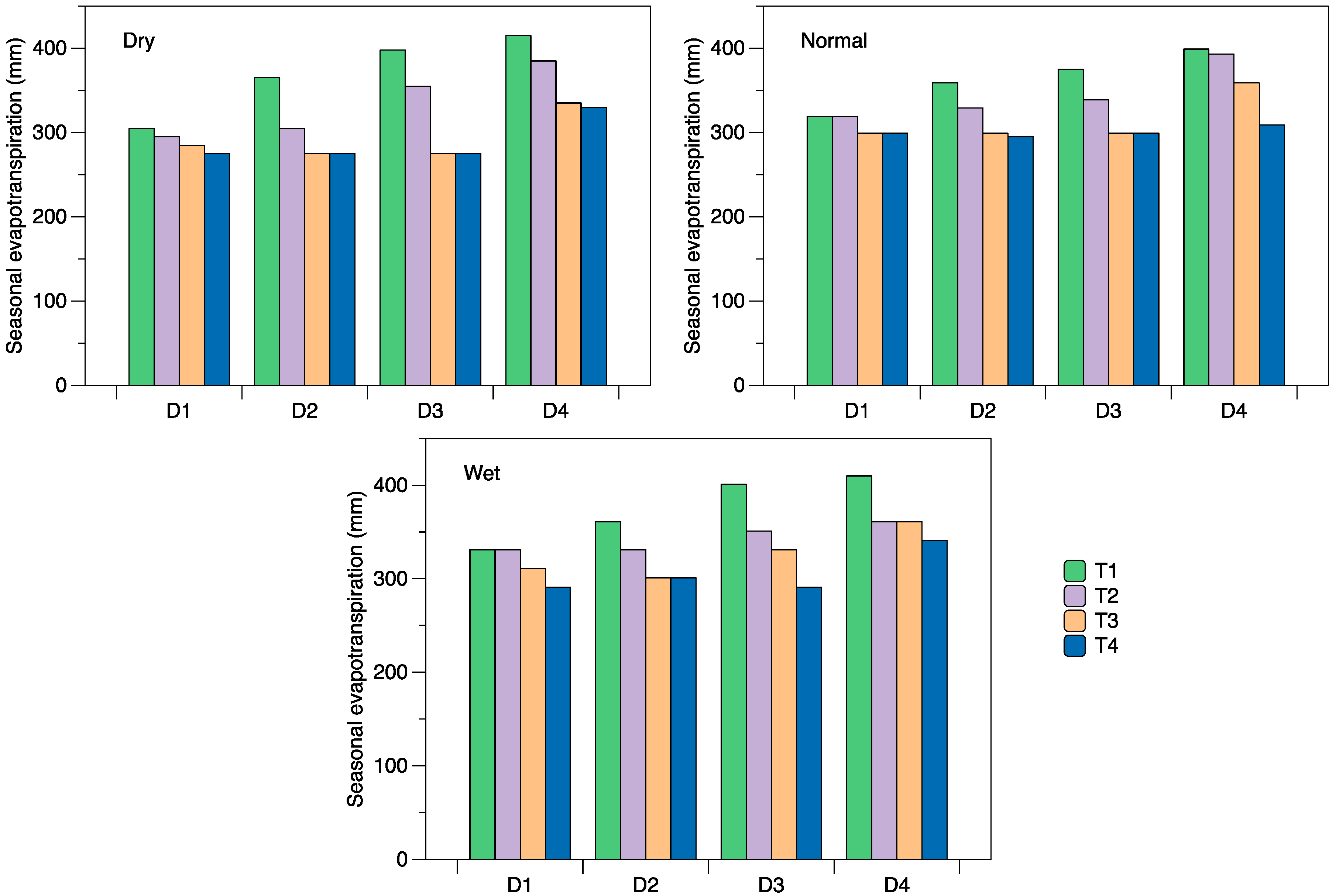
3.2. Simulated Crop Evapotranspiration
Figure 4 shows the simulated seasonal evapotranspiration (ET) for the different water application depths for the depletion irrigation scheduling. Across the three characteristic seasons, seasonal ET for the different schedules ranged from 305 to 415 mm for T1, 295 to 393 mm for T2, 275 to 361 mm for T3 and 275 to 341 mm for T4. These simulated values fall within the range of seasonal consumptive water use reported in other simulation studies for maize [
12,
14] and some deficit studies observed through field experimentation [
26]. However, the lower values appear to be outside (below) the range of other field studies [
27,
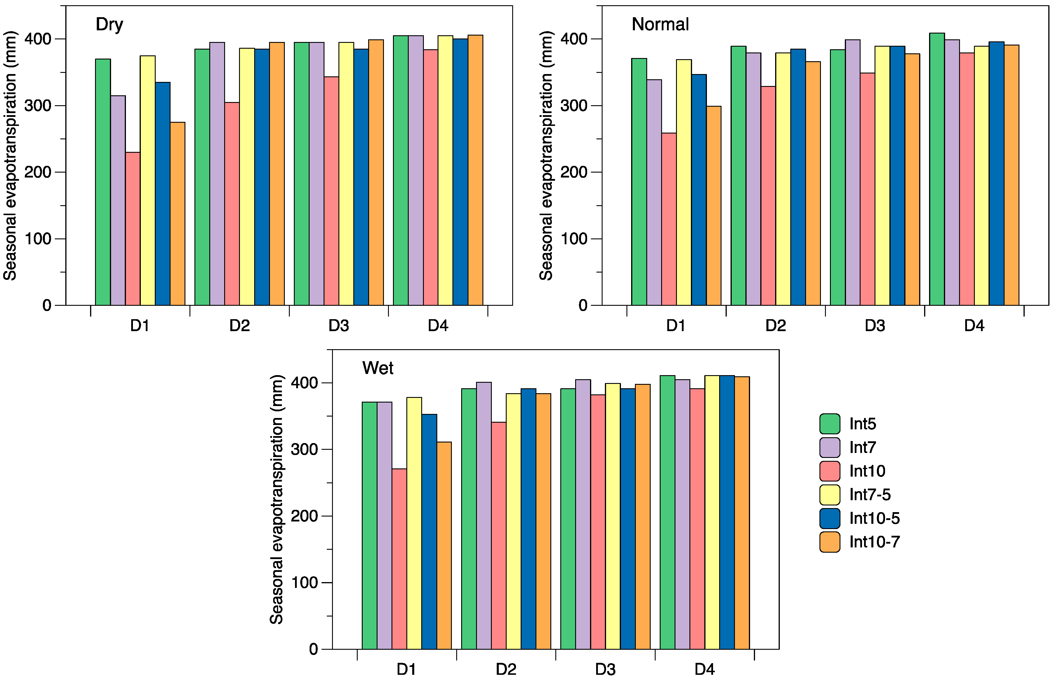
28]. Higher ET values were observed for lower depletion schedules and larger water application depths, indicating that these treatments were less susceptible to water deficits. The variation in simulated ET for the interval schedules and water application depths across all characteristic seasons is depicted in
Figure 5. For the three characteristic seasons, the lowest ET values were observed for the Int10 schedule ranging from 230 to 391 mm followed by the Int10–7 schedule with a range of 275 to 411 mm. The simulated ET for the four remaining schedules was within the range of 315 to 411 mm. The two-way ANOVA results indicated that overall, the variation in simulated ET was highly significant at the 1% level for all characteristic seasons for the various depletion (Tn) and interval schedules (Intn), while the mean ET associated with the water application depths (Dn) were significantly different at 5%. However, similar to the results reported by Igbadun and Salim [
14], no significant interaction effects were observed in either irrigation scheduling scenario, implying that the variation was not a result of the combined effect of the depletion levels and water application depth or interval schedules and water application depth. Further analysis revealed that the mean ET was significantly different among some groups (
Tables S1 and S2). In particular, highly significant differences were observed for T1 scheduling compared to the other Tn schedules (
Table S1). Additionally, in terms of water depths, the only significant difference observed was for D4 compared to the water depths D1 and D2. With regards to the different scheduling intervals, the mean ET for Int10 was significantly different from Int5, Int7, Int7–5 and Int10–5 across the dry and normal characteristic seasons, while for the wet season, Int10 was significantly different only for Int5, Int7 and Int7–5 (
Table S2). For the other schedules, Tukey’s test statistic indicated that there was no significant difference. As regards the water depths, significant differences were observed for D1 compared to all other water depths across all three characteristic seasons (
Table S2).
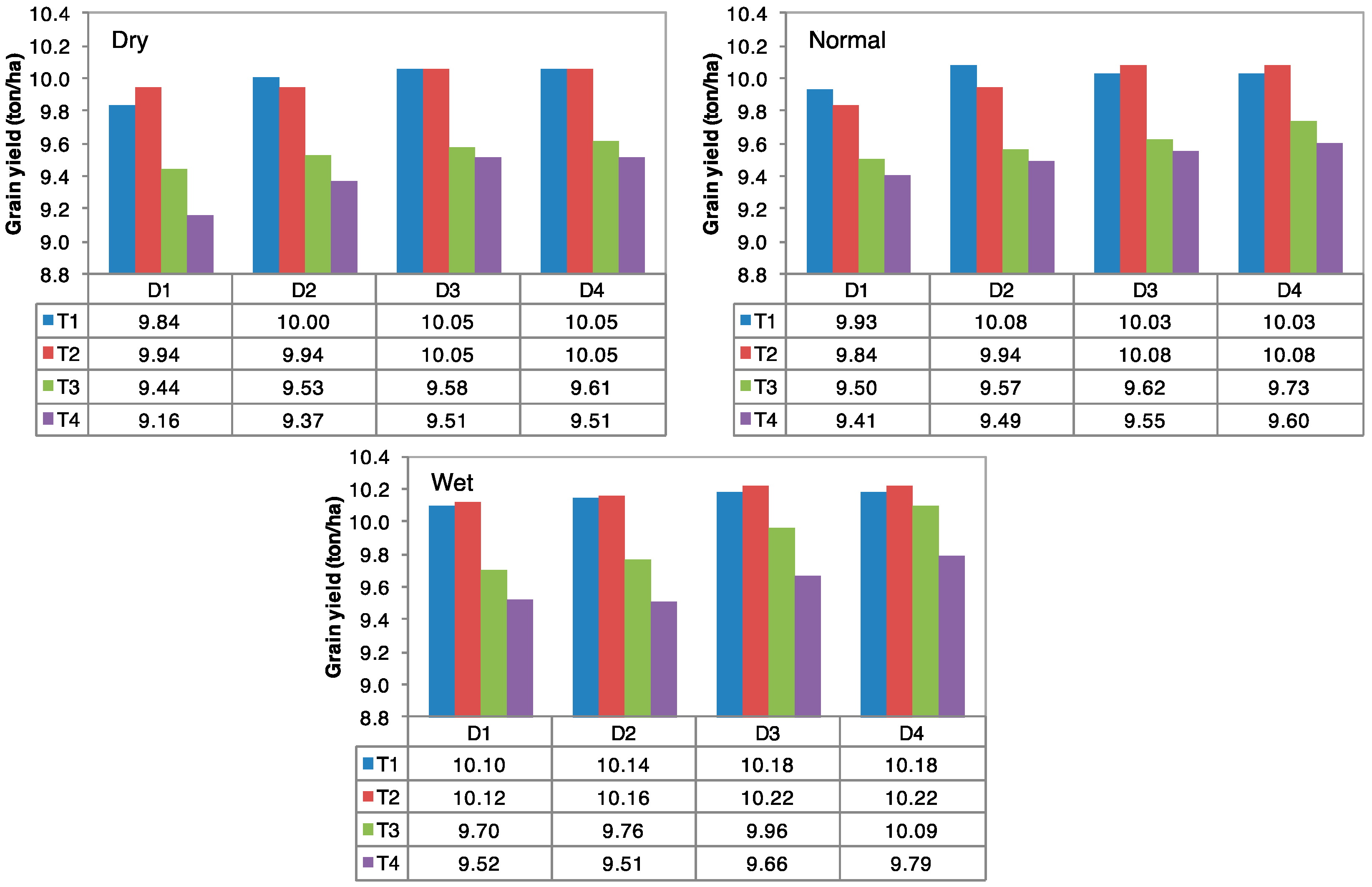
3.3. Simulated Grain Yield
Simulated yields for the different depletion levels and water application depths for the three characteristic seasons of water availability are presented in
Figure 6. In a dry, normal and wet season, the simulated yields ranged from 9.16 to 10.05 ton/ha, 9.41 to 10.09 ton/ha and 9.51 to 10.22 ton/ha, respectively. The yields obtained in this simulation study are within the range reported for the study area based on field experiments [
18]. Irrigation based on the lower depletion levels typically produced higher yields than the higher depletion levels (
Figure 6). In general, the highest yields were obtained when irrigation water application depth was at least 40 mm for schedules T1 and T2. Further, as can be observed from the figure, in most cases, there is no considerable difference between the yields obtained for T1 and T2 scheduling, indicating that the increase in irrigation application did not result in an appreciable increase in productivity, presenting opportunities for water savings. Simulated water application for T1 was considerably higher at these water depths (
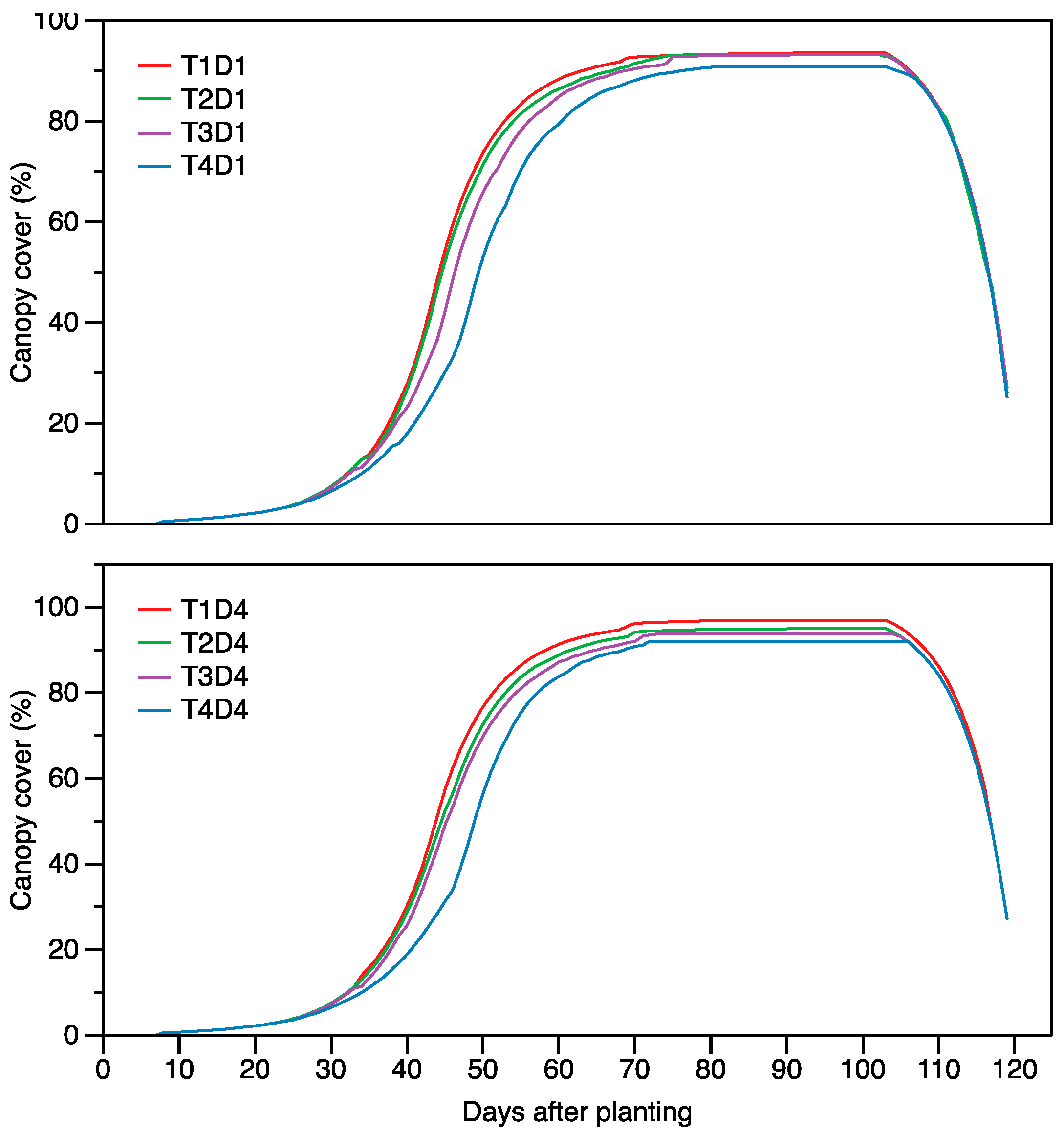
Figure 2). Deep percolation losses for some of these treatments further suggest that the crop was over-irrigated. In addition, for the wet characteristic season, there was also no substantial reduction in the simulated yield of T3D3 and T3D4 compared to the maximum yields observed in T1 and T2, indicating that utilizing a water depth of 40–50 mm at a 50% depletion of TAW in the root zone is a viable strategy to consider for this climate scenario. Here, a reduction of 2.5% and 1.29% for these two strategies was observed respectively. In the study, AquaCrop simulation output for biomass ranged from 19.96 to 20.73 ton/ha, 20.16 to 20.64 ton/ha and 20.43 to 20.57 ton/ha for the dry, normal and wet characteristic seasons. The impact of the different irrigation strategies on crop growth under the depletion irrigation scheduling method is illustrated in
Figure 7 for selected strategies. The ANOVA test indicated that overall, there was a significant difference (
p < 0.05) among the mean grain yield for the different depletion schedules and for the varying water application depths for all characteristic years. Further analyses revealed that generally, the mean grain yields were not significantly different when the water application was above 30 mm (D2) (
Table S1). Contrastingly, the difference in simulated yields was significant among most of the schedules, especially for the wet season.
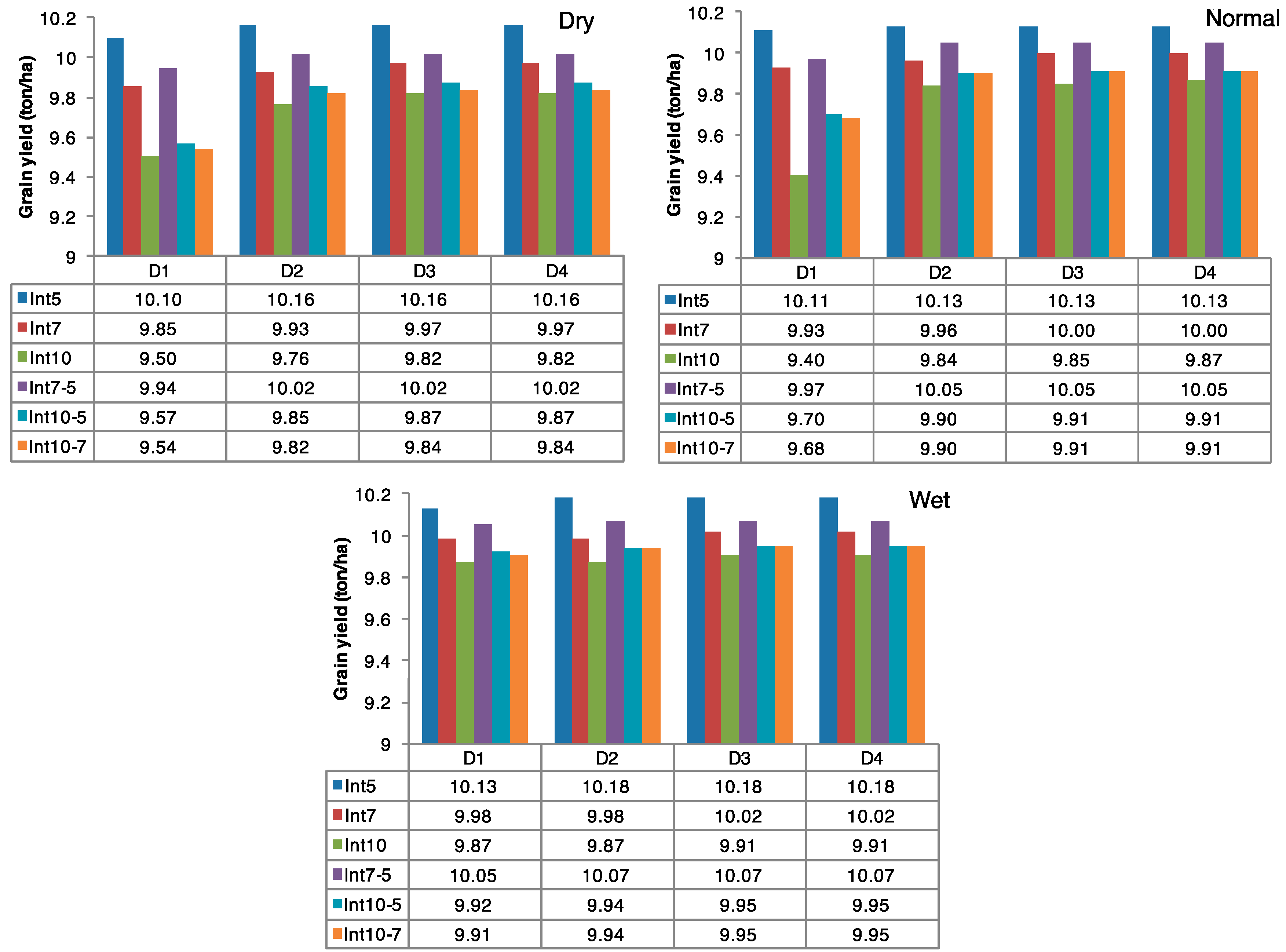
Figure 8 presents the yield simulated in AquaCrop for the different interval schedules at various water application depths. Across the three characteristic seasons, the yield for the schedules Int5, Int7, Int10, Int7–5, Int10–5 and Int10–7 were within the range of 10.10 to 10.18 ton/ha, 9.85 to 10.02 ton/ha, 9.40 to 9.92 ton/ha, 9.94 to 10.07 ton/ha, 9.57 to 9.95 ton/ha and 9.54 to 9.95 ton/ha. Higher yields were generally observed in the wet characteristic season. The relative reduction in yield for the dry, normal and wet characteristic season, estimated from the maximum simulated yield in each season, varied from 0.62% to 6.52%, 0.22% to 7.1% and 0.48% to 3.18%, respectively. The lowest yields and thus highest percent reduction were observed in the Int10 schedule, whilst the maximum yield was observed in the Int5 schedule. Two-way ANOVA testing revealed that overall, there was a significant difference in mean yield for the different interval schedules and for the varying water application depths for all characteristic seasons. The result of Tukey’s significance test revealing groups in which the yields were significantly different is presented in
Table S2. As with the simulated ET, a significant difference was observed for D1 compared to all other water depths across the three characteristic seasons. Considering the interval schedules as the factor, the higher yields simulated in the Int5 schedule were significantly different from the yields simulated in most of the other schedules (
Table S2). For the remaining comparisons, significant differences for the mean yields for the dry and normal seasons were observed between only a few of the other interval schedules. In contrast, for the wet season, the mean yield was significantly different across the remaining comparisons, except Int10–5 vs. Int10–7.
3.4. Crop Water Productivity
Table 1 shows the simulated crop water productivities for the different irrigation strategies under the depletion scheduling method in terms of seasonal water applied (WUE
Irr) and crop consumptive use (WUE
ET), estimated as yield per unit total irrigation water supplied and ET
c, respectively. In general, the WUE
Irr was higher during the wet season, as less water was supplied to meet crop water requirements, and increased as the depletion criterions increased, since water application was less frequent. Furthermore, estimated values in the table show that in most cases, there was no considerable difference between the values for the depletion schedules T3 and T4 for the dry and normal characteristic seasons. During the characteristic dry season, WUE
Irr ranged from 2.01 kg/m
3 in T1D4 to 3.99 kg/m
3 in T3D2 and T3D3; for the characteristic normal season, the values ranged from 2.23 kg/m
3 in T1D4 to 4.01 kg/m
3 in T3D3; while for the wet season, WUE
Irr ranged from 2.26 kg/m
3 in T1D4 to 4.83 kg/m
3 in T4D3. Similarly, for the three characteristic seasons, the minimum and maximum WUE
ET were observed in the same combinations with ranges of 2.42–3.48 kg/m
3, 2.51–3.22 kg/m
3 and 2.48–3.32 kg/m
3 for the dry, normal and wet seasons, respectively (
Table 1). The percent relative change in WUE
ET for each strategy compared to the maximum WUE
ET observed for the specific characteristic season is also presented in the table. The values on the lower end of this relative scale indicate that there is no substantial difference between the maximum WUE
ET and the values observed in the respective strategy, implying that these strategies offer opportunities for improving water use. Specifically, utilizing a depletion schedule of 50% (T3) and 60% (T4) for initiating irrigation offers opportunities for water saving, as more than 50% of the values had a relative change of less than 5%. Further, a depletion schedule of 40% (T2) can improve crop water productivity in irrigated maize production when using water application depths of 20 (D1) mm and 30 (D2) mm; the relative change for these combinations compared to the maximum WUE
ET is less than 9%. Higher relative changes (lower WUE
ET values) for the remaining combinations for this depletion schedule (T2D3 and T2D4) indicate that the increase in water application (
Figure 2) did not result in an appreciable increase in grain yield.
Estimated WUE
Irr for the interval scheduling method is displayed in
Table 2. As can be observed, the WUE
Irr decreased with increasing water depths. Furthermore, considering the various combinations, in most cases, the variation in values between the three seasons was small. This can be attributed to the fact that the interval scheduling employed resulted in the same amount of irrigation water being supplied across the three seasons. For the three characteristic seasons, the highest values were observed in the Int10 schedule ranging from 2.18 kg/m
3 to 5.48 kg/m
3, which was expected given the lower amounts of irrigation water supplied. Across the three characteristic seasons, the mean relative reduction in WUE
Irr for the schedules Int5, Int7, Int7–5, Int10–5 and Int10–7 compared to the maximum WUE
Irr observed in the respective Int10Dn combination was 51%, 35%, 46%, 40% and 24%, respectively. A greater disparity in WUE
ET (
Table 3) values between seasons was observed for the different simulations compared to the values in WUE
Irr (
Table 2). However, the difference was less pronounced at the higher water depths of D3 and D4. Again, higher WUE
ET values were obtained for the Int10 schedule. For the dry characteristic season, the relative reduction in WUE
ET for Int5, Int7, Int7–5, Int10–5 and Int10–7 compared to the maximum WUE
ET observed in the respective Int10Dn combinations was within the range of 2–38%, 4–29%, 3–40%, 4–35% and 5–21%, respectively. For the normal characteristic season, the relative reduction for the respective combinations was within the range of 5–31%, 4–26%, 1–31%, 4–29% and 3–18%. Additionally, the relative reduction for the respective combinations for the wet characteristic season ranged from 2–25%, 2–26%, 3–37%, 4–23% and 4–13%. In the dry, normal and wet season, 7, 8 and 12 cases (out of 20), respectively, recorded less than or equal to 10% reduction in WUE
ET compared to the maximum WUE
ET simulated for the respective IntnDn combinations.
Comparison between the numerical outputs of yield and WUE
Irr and WUE
ET generally informs about the suitability of irrigation strategies for improving agricultural water productivity [
3]. For a characteristic dry/normal season, high yields and high WUE
Irr and WUE
ET observed for the following combinations indicate practical schedules for water savings without significant yield penalty: T2D1, T2D2, T3D1, T3D2 and T3D3. Considering a wet season, feasible schedules include T2D1, T2D2, T3D1, T3D2, T3D3, T4D2 and T4D3. Although a depletion of 50–55% is typically recommend [
24], the results indicate that a depletion schedule of 60% (T4) with large water application depths is viable for this location for priorities of improving agricultural water use. Of course, in water scarcity conditions, the lower water application depths should be used. The results also indicate that although utilizing a depletion schedule of 30% (T1) resulted in high yields, the lower WUE
Irr and WUE
ET (except for a 20 mm (D1) depth (
Table 1)) imply that the higher water application amounts (
Figure 2) did not result in a substantial increase in productivity; thus, utilizing this schedule is not sustainable towards the goal of water saving. Further supporting this is the observation that the simulated yields for T1 were not significantly different from those simulated in T2 (
Table S1). As regards the irrigation scheduling interval method, utilization of the schedule Int7–5 at water application depths of 40 (D3) and 50 (D4) mm for the dry and normal seasons and depths of 30 (D2) to 50 (D4) mm for the wet season can be used. In these cases, both the relative reduction in yield (<1.5%) and WUE
ET (<10%) compared to the maximum were among the lowest. The schedules Int10–5 and In10–7 at depths of 30 to 50 mm resulting in less than 4% reduction in yield and less than 12% change in WUE
ET compared to the maximum for both the wet and normal years are also feasible strategies. On this relative basis, the schedule Int10–5 for depths of 40 mm and 50 mm can be utilized for a dry characteristic season. Considering however the simulated deep percolation, high water losses observed for higher water depths suggest that the lower depths in the aforementioned cases should be employed. Further, it should be noted that for these three aforementioned schedules, a water depth of 20 mm (D1) can also be used, especially considering that the lowest percolation losses (ranging from 0–21% across all three characteristic seasons and the various schedules) were obtained at this water depth, but a significantly higher yield penalty is to be expected. Highly significant differences (
p < 0.01) were observed between D1 and depths D2 to D4 on yield (
Table S2). Although the highest WUE
ET and WUE
Irr were observed for the Int10 schedule, a higher yield penalty would be a limiting factor to its practicality. However, as the lowest water losses to deep percolation were observed for this schedule, it can be a viable strategy especially for a projected wet characteristic season. Similarly, although the highest yields were generally observed in the Int5 schedule, low WUE
ET suggests that the feasibility of this strategy for sustainable use of water resources is inadequate. Furthermore, high percolation losses associated with this schedule supports this. In using ISIAMod (Irrigation Scheduling Impact Assessment Model), Igbadun and Salim [
11] and Igbadun et al. [
25] also illustrated that using a five-day interval schedule does not benefit agricultural productivity in terms of yield and water productivity.


