Responses of Vegetation Growth to Climatic Factors in Shule River Basin in Northwest China: A Panel Analysis

Abstract

The vegetation response to climatic factors is a hot topic in global change research. However, research on vegetation in Shule River Basin, which is a typical arid region in northwest China, is still limited, especially at micro scale. On the basis of Moderate-resolution Imaging Spectroradiometer (MODIS) Normalized Difference Vegetation Index (NDVI) data and daily meteorological data, employing panel data models and other mathematical models, the aim of this paper is to reveal the interactive relationship between vegetation variation and climatic factors in Shule River Basin. Results show that there is a widespread greening trend in the whole basin during 2000–2015, and 80.28% of greening areas (areas with vegetation improvement) are distributed over upstream region, but the maximum vegetation variation appears in downstream area. The effects of climate change on NDVI lag about half to one month. The parameters estimated using panel data models indicate that precipitation and accumulated temperature have positive contribution to NDVI. With every 1-mm increase in rainfall, NDVI increases by around 0.223‰ in upstream area and 0.6‰ in downstream area. With every 1-°C increase in accumulated temperature, NDVI increases by around 0.241‰ in upstream area and 0.174‰ in downstream area. Responses of NDVI to climatic factors are more sensitive when these factors are limiting than when they are not limiting. NDVI variation has performance in two seasonal and inter-annual directions, and the range of seasonal change is far more than that of inter-annual change. The inverted U-shaped curve of the variable intercepts reflects the seasonal change. Our results might provide some scientific basis for the comprehensive basin management.

1. Introduction

Vegetation, the main component of the terrestrial biosphere, is a crucial element in the climate system [1]. Its variation is an important indicator of regional changes in ecology and environment [2]. Understanding the relationship between the greenness of vegetation and climate is an important topic in global change research [3]. The vegetation in the arid regions in west China, which is a sensitive and fragile ecological zone, has a sensitive response to the global climate change. Therefore, this region becomes one of the key areas for studying global environmental changes [4]. Normalized Difference Vegetation Index (NDVI) is one of the main characteristic descriptors of vegetation cover and is widely used to monitor the changing dynamics of vegetation cover, biomass and the ecosystem [5]. In addition, NDVI can be used to represent the proxy vegetation responses to climate changes since it is well correlated with the fraction of photosynthetically active radiation absorbed by plant canopies and thus leaf area, leaf biomass and potential photosynthesis [6].

In the latest 30 years, there have been many research studies conducted on the relationship between vegetation activity and its driving factors. The global vegetation presents an obvious greening trend [7,8,9,10,11,12,13], especially in middle and high latitudes of the Northern Hemisphere [7,8,10,11]. Despite great spatial heterogeneity, vegetation greenness in arid and semi-arid regions on average experienced an increase in both global [4,14] and regional scale, for example, in Central Asia [15,16], Inner Asia [17], Eurasia [18], Sahel [19], and Australia [20]. The greening trend also appears in the Tibet Plateau and the arid regions in northwest China [21,22,23,24,25,26,27].

Potential drivers of vegetation change can be divided into two categories: natural and human factors. Natural factors include temperature, precipitation, photosynthetically active radiation, atmospheric concentrations of CO₂, etc. [18,28]. Human factors mainly include cultivation, afforestation, deforestation, urbanization as well as improved agricultural management practices [18,28,29]. Generally, large scale variations are affected by climatic factors that represent the dominant limitation to plant growth [20]. Elevated air temperature and increased water availability are the dominant climatic factors [28,29,30,31,32,33,34,35,36,37]. Shule River Basin is a typical arid region in northwest China and is strongly disturbed by human activities. Compared with related research about Shiyang river basin and Heihe river basin in the Hexi region, research about Shule River Basin is very limited. On the basis of MODIS NDVI data with 250-m spatial resolution and daily meteorological data, this article employed panel data models to analyze the vegetation dynamic and its response to climate change from 2000 to 2015. Our purpose is to reveal the characteristics, trend and spatio-temporal difference of vegetation change, and to quantify impacts of climatic factors on NDVI, which might provide some scientific basis for the comprehensive basin management.

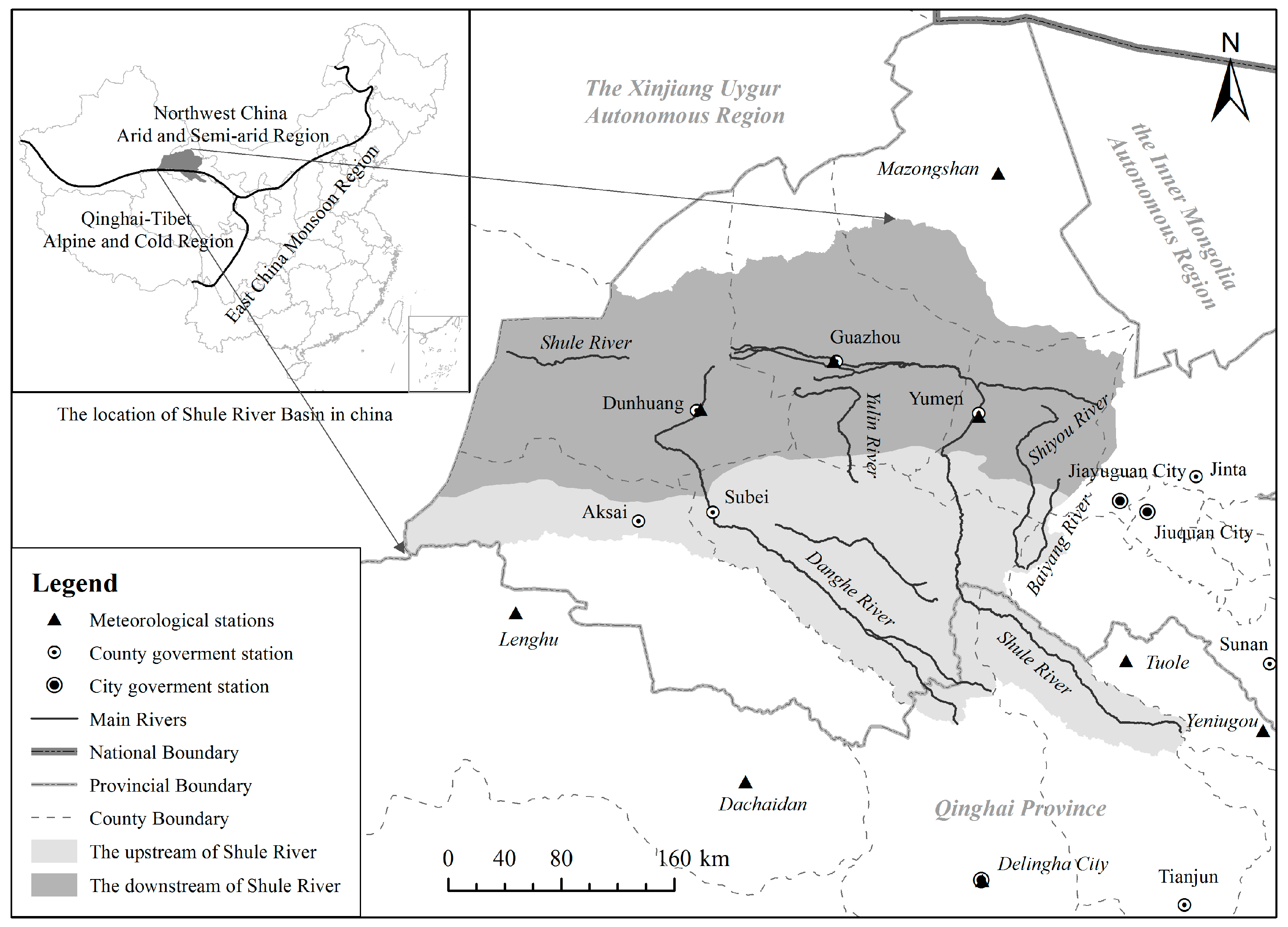
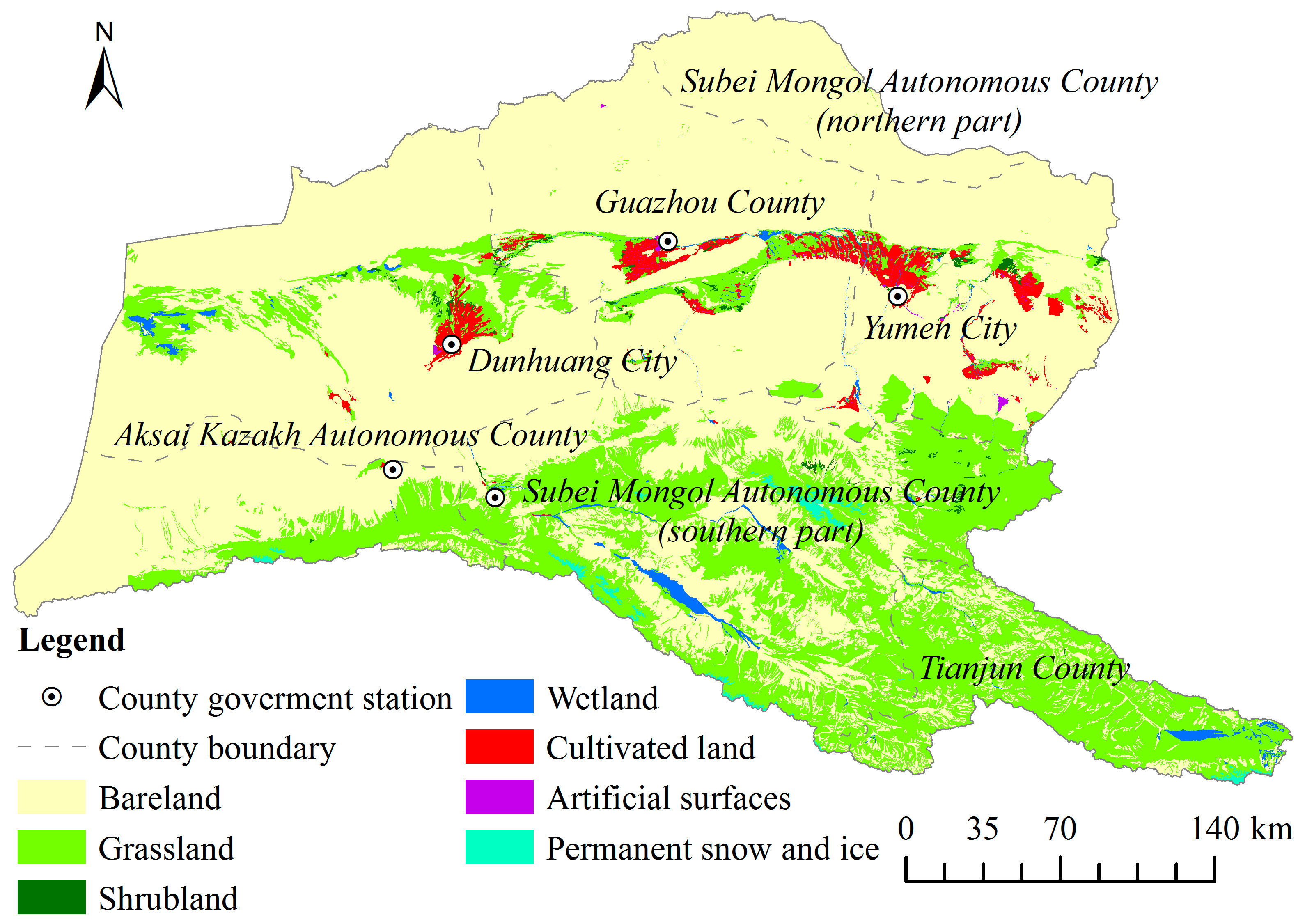
2. Overview of the Study Region

Shule River Basin with an area of 100,000 km² is located in inland area of northwest China (92.33°–98.99° E, 38.21°–41.47° N) (Figure 1). Its southern part is the Qilian Mountains with an average elevation of 3.49 km, where the Shule River originates. Its northern part is low mountainous region with an average elevation of 1.95 km, which is called Mazong Mountains. Its middle part is the flat Hexi Corridor with an average elevation of 1.4 km, where Huahai, Yumen and Dunhuang-Anxi basin are distributed from east to west. Oasis and population are mainly distributed over this part. Because of being situated in the hinterland of Asia-European continent, the Shule River Basin is characterized by an arid climate, little rainfall and sparse vegetation. The mean annual temperature ranges from 0 °C to 10 °C, and the mean annual precipitation is about 100 mm. The cold steppe, temperate steppe and desert steppe in turn are distributed over Shule River Basin from Qilian Mountains to Hexi corridor and to north hills. Generally, Shule River Basin is a region with fragile ecological system, and response of vegetation growth to climatic change in this region is very sensitive.

In addition, the vegetation growth in Shule River Basin is affected by human activity. The ancient Silk Road passes through this region to Central Asia. Dunhuang Mogao Caves, a world-famous cultural heritage, is located in the western end of the Hexi corridor. At present, all trunk railways and highways linking China and Central Asia pass through this region. Moreover, there are many wind farms and photovoltaic plants running in Yumen city, which is the cradle of China’s oil industry. In the late 1980s, the government of Gansu Province implemented Shule River Basin Agricultural Irrigation and Immigration Development Projects with a grant from World Bank, and more than 100,000 people were moved there during resettlement as part of “China Western Development” government policy. This resulted in a rapid increase in agricultural acreage and irrigation water use, which had a considerable influence on local environment. From 1985 to 2014, population grew from 372,700 to 526,400 and total cultivated area increased from 48,600 hm² to 91,390 hm². The irrigated agriculture in oasis caused large consumption of water resources and diverted water previously used by the natural environment. Therefore, it is very essential to strengthen surveillance of environmental change in Shule River Basin.

The existing studies on vegetation variation in Shule River Basin focus on two aspects: Land-use and land-cover change (LUCC) and trend of vegetation index. To be more specific, some of the existing studies use Landsat data to investigate LUCC classification, landscape pattern change, driving mechanism, dynamic process modeling and ecological environment effect. Restricted by temporal resolution of Landsat data, the available cross-section data are limited. Thus, there are often some differences among different research results. On the basis of NDVI data acquired by Advanced Very High Resolution Radiometer (AVHRR) [38], Systeme Probatoire d’Observation de la Terre (SPOT) [39] and Moderate-resolution Imaging Spectroradiometer (MODIS) [40], other existing studies mainly analyzes changes in NDVI [41] and net primary productivity (NPP) [42] and their response to climatic change. These studies usually detect vegetation variation in Shule River Basin at macro scale; however, micro-scale study on Shule River Basin is scarce. In addition, because of lower spatial resolution of data that are employed by previous research, it is hard to obtain good results in the study of Shule River Basin with sparse vegetation cover.

3. Data Sources and Methodology

3.1. Data Sources and Processing

At present, common NDVI dataset is mainly acquired from AVHRR, MODIS and SPOT satellite platform [43]. Among them, AVHRR gives the longest time series of NDVI (from 1981), but with lowest spatial resolution (8 km), whereas SPOT and MODIS give shorter time series of NDVI (from 1998 and 2000, respectively), but with higher spatial resolution. Compared with AVHRR and SPOT data, MODIS data have better quality, better timeliness and higher availability. Furthermore, considering the feature of sparse vegetation cover in Shule River Basin, we chose to use MODIS data. The data used in this article come from three sources. (1) MODIS NDVI and its Pixel Reliability data are from Level-1 and Atmosphere Archive & Distribution System (LAADS) WEB, with numbers h25v04 and h25v05, a 250-m spatial resolution and 16-day temporal resolution. The period is from 2000 to 2015, and there are a total of 1460 images in 365 stages, each year in the study period has 23 phases, and each phase includes 16 days. The data were transformed into World Geodetic System 1984 (WGS 1984) and converted into Geotiff format. (2) Digital Elevation Model (DEM) data with 90-m spatial resolution are acquired from geospatial data cloud web. (3) Meteorological data are acquired from China meteorological data network.

Influenced by incident angles of sunlight, clouds, aerosols and sensor capability, NDVI data contain some noise, which results in irregular fluctuations in time series [44]. Thus, it is necessary to perform de-noising. Previous research has shown that the Asymmetric Gaussian (A-G) algorithm can effectively decrease the noise for the arid area and achieve high fidelity of original data [45]. To de-noise, we took the MODIS quality evaluation data as weight and fitted NDVI data pixel by pixel using TIMESAT soft in accordance with A-G method. The value of NDVI ranges from −1 to 1, and NDVI ≤ 0 is generally considered to denote no vegetation cover. However, influenced by soil background, the threshold value is usually greater than zero and changes with different underlying surfaces [46]. To get reasonable threshold value that is suitable for Shule River Basin, the yearly average values of NDVI from May to October (NDVI_5–10) were calculated. Then, maximum value of NDVI_5–10 (MAXNDVI_5–10) during 2000–2015 was obtained. Using the vegetation information obtained from Landsat Thematic Mapper (TM) images, which has a high spatial resolution of 30 m, we considered MAXNDVI_5–10 ≥ 0.12 is an appropriate threshold value that denotes vegetation in Shule River Basin. On the basis of this, we performed masking on all images.

3.2. Research Methodology

3.2.1. Linear Trend Analysis

Change in NDVI over time could be expressed as the following regression equation [47]:

$$y_i=\theta i+bi=1,2,3,\cdots ,n$$

(1)

where y_i is the NDVI value in ith year, b is the intercept, n is the number of years in the study period, and θ is the slope representing linear trend of NDVI change, which is estimated by the least square method. Positive θ suggests that vegetation coverage increases with time, whereas negative θ indicates vegetation coverage decreases with time. t test can provide statistical confidence level for variations in NDVI.

3.2.2. Multiple Correlation Analysis

In multi-factor system, the multiple correlation coefficient R_z∙xy reflects the level of association among three or more random variables (Equation (2) takes three variables as example) [48].

$$R_{z\cdot xy}=\sqrt{1-(1-r_{zx}^2)(1-r_{zy\cdot x}^2)}$$

(2)

where r_zx is the simple correlation coefficient between variable z and x, and r_zy∙x is the partial correlation coefficient between variable z and y while the effects of the variable x are controlled.

3.2.3. Mann–Kendall (M-K) Trend Detection

M-K method is a non-parametric test for assessing the significance of a trend [49,50]. If {x_t} is a time series with n samples, statistics S can be defined as follows:

$$S={\displaystyle \sum _{i=1}^{n-1}{\displaystyle \sum _{j=i+1}^{n}sgn(x_j-x_i)}}$$

(3)

$$sgn(x_j-x_i)=\{\begin{array}{c}1\\ 0\\ -1\end{array}\begin{array}{c}{x}_j>x_i\\ x_j=x_i\\ x_j<x_i\end{array}$$

(4)

The standardized test statistic (Z) of the M-K test is given by Equation (5), which follows the standard normal distribution, and the corresponding significance level (α) of two-tailed test can be confirmed when |Z| ≥ Z_1-α/2 [49,51].

$$Z=\{\begin{array}{cc}(S-1)/\sqrt{n(n-1)(2n+5)/18}& S>0\\ 0\hfill & S=0\\ (S+1)/\sqrt{n(n-1)(2n+5)/18}& S<0\end{array}$$

(5)

$$\beta =median\left[(x_j-x_i)/(j-i)\right]i<j$$

(6)

where β is the estimate of the trend and x_j is the jth observation, which indicates the magnitude of a trend. Positive Z value indicates an increasing trend while negative Z value indicates a decreasing one [51].

3.2.4. Panel Data Regression

Panel data analysis is an econometric model that is widely used in social and economic fields. It can make full use of the information contained in the samples and reflect the trends of research objects in three dimensions (cross-section, period and variables) [52]. In this article, we took the 23 phases in a year as a cross section of individuals, and revealed the characteristics of interaction between variables. To confirm the validity of parameter estimation, it is necessary to test stationarity of time series before establishment of the panel regression model [53]. Here, we employed five panel unit root tests (LLC, Breitung, IPS, Fisher, and HT) to confirm the stationarity of variables [53]. There are many types of models for the panel regression analysis, and the basic model is as follows:

$$y_{it}=\alpha +\beta x_{it}+u_{it}\hspace{1em}(i=1,2,\cdot \cdot \cdot ,N;t=1,2,\mathrm{...}T)$$

(7)

where N and T is the number of phase and year, respectively. We assumed that the impact of climatic factors on NDVI is unrelated to phases, which means α₁ = α₂ = … = α_N in Equation (7). If coefficient β is also constant, Equation (7) is called the pooled regression model (H₁). If β is constant while α_i changes over phase, Equation (7) is called the variable intercept model (H₂). The variable coefficient model accepts neither assumptions H₁ nor H₂.

4. Results

4.1. Quantity Characteristic of Vegetation Coverage

The average value of MODIS NDVI from 2000 to 2015 over a 16-day interval in Shule River Basin is acquired using ArcGIS software (Environmental Systems Research Institute Incorporation, Redlands, CA, USA). The growing season of vegetation begins on 113th day of the year and ends on 320th day of the year, with a length of 208 days (Figure 2). The peak of NDVI appears in the end of July. Changing curve in downstream area shows a higher NDVI value than that in upstream area, and both curves have inverted-U shapes (Figure 2). The yearly average NDVI during growing season (NDVI_gs) shows a linear uptrend over the years, especially in the downstream area (Figure 3). This result is consistent with some existing study [54].

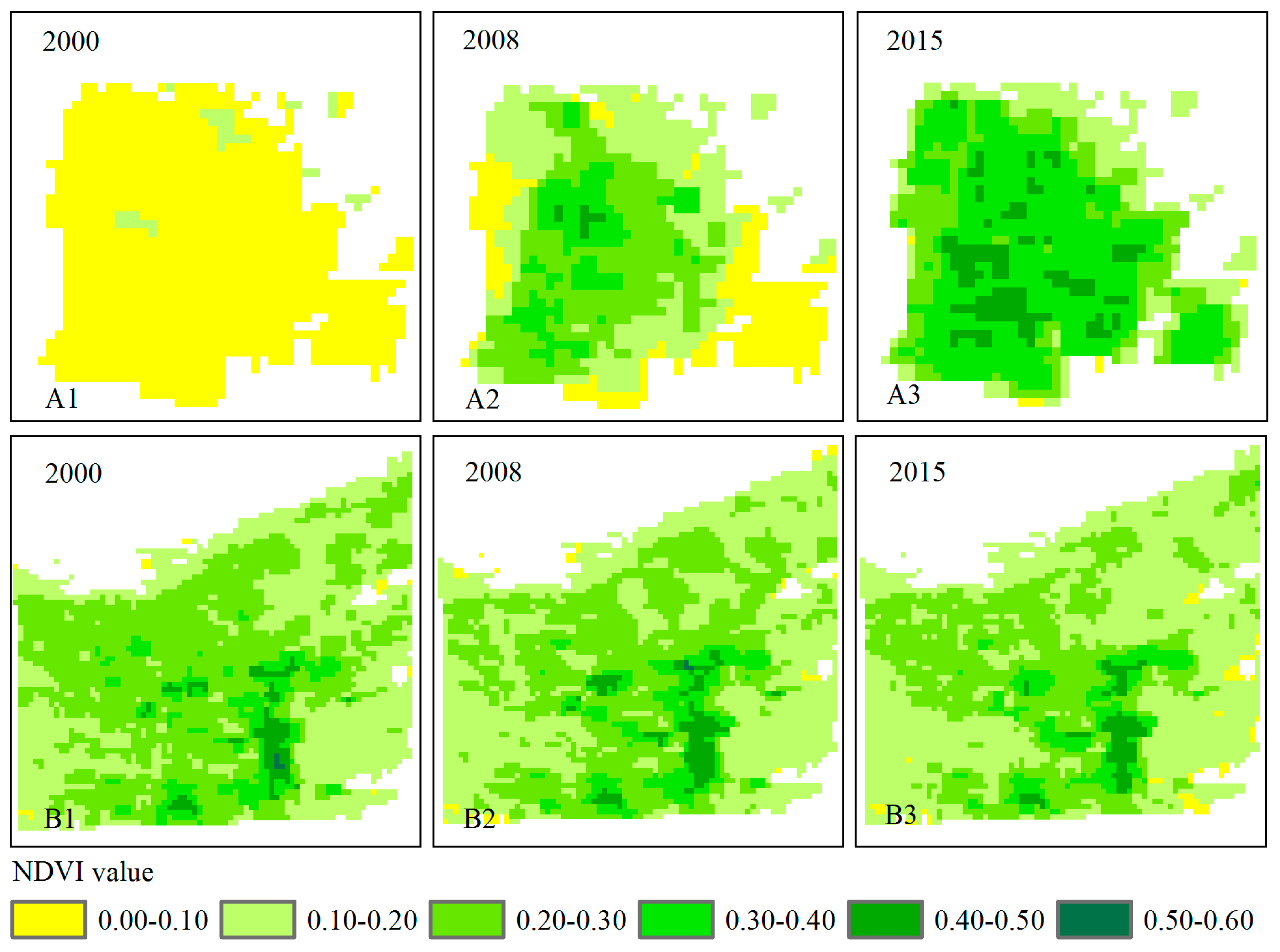
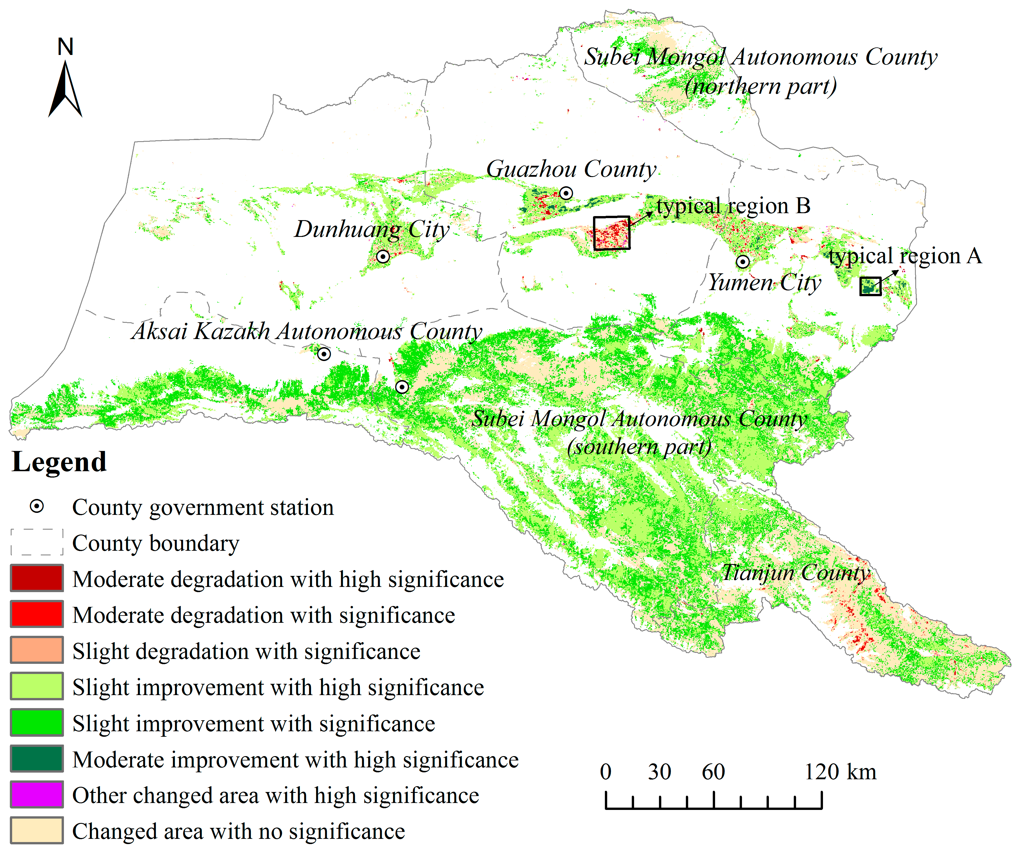
4.2. Spatial Characteristics of Vegetation Change

θ values in Equation (1) are calculated pixel by pixel and divided into six types, and analyzed with t test under three significance levels, as shown in

Table 1. Proportions (%) of areas with different NDVI_gs trends under different significance levels (2000–2015).

NDVIgs Trends	High Significance p ≤ 0.01	Significance 0.01 < p ≤ 0.1	No Significance p > 0.1	Summary
Moderate degradation (−0.03 < θ < −0.02)	0.4363	0.5849	0.2585	1.2797
Slight degradation (−0.02 ≤ θ < 0)	0.0569	0.4376	5.4947	5.9892
No change (θ = 0)	-	-	0.0283	0.0283
Slight improvement (0 < θ < 0.02)	31.254	32.2391	28.7498	92.2429
Moderate improvement (0.02 ≤ θ < 0.04)	0.4597	-	-	0.4597
High improvement (0.04 ≤ θ < 0.05)	0.0002	-	-	0.0002
Summary	32.2071	33.2616	34.5313	100

. There exists a specific θ value in each grid with vegetation, and all θ values marked in the raster map constitute the spatial pattern of vegetation cover (see Figure 4). The color white means the parts without vegetation cover in Figure 4. There are great variations in θ values under three test levels, which exhibit the spatial heterogeneity of NDVI_gs.

The area with slightly improved NDVI_gs accounts for the largest portion of total area (92.24%), which indicates the general trend of vegetation in Shule River Basin. The area with slightly degraded NDVI_gs accounts for the second largest portion of total area (5.99%). Areas with other types of vegetation change account for only a small percentage. The t test results show that the proportions of area with different kinds of vegetation changes at high significance, significance and no significance levels are 32.21%, 33.26% and 34.53%, respectively. The area with slightly degraded NDVI_gs under no significance level accounts for 91.74% under all levels. Generally, the vegetation coverage has increased during 2000–2015 in most areas of Shule River Basin, and areas with vegetation degradation only accounts for small proportion (less than 8%).

The greening areas, that is, areas with slightly, moderately or highly improved NDVI_gs, accounts for 92.70% of the total areas (Table 1). Among them, 69.45% are distributed over upstream region, Aksai Kazakh Autonomous County, Subei Mongol Autonomous County (southern part) and Tianjun County account for 8.87%, 44.74% and 15.84%, respectively (see

Table 2. Areas percentages of different NDVI_gs trends (2000–2015) among different counties.

	Degradation (θ < 0)	No Change (θ = 0)	Improvement (θ > 0)	Summary
Guazhou	1.41	0.00	5.88	7.29
Dunhuang	0.62	0.00	4.26	4.87
Yumen	0.97	0.00	9.09	10.06
Tianjun	3.09	0.01	15.84	18.94
Subei (southern part)	1.01	0.01	44.74	45.76
Subei (northern part)	0.14	0.00	4.03	4.17
Aksai	0.03	0.00	8.87	8.90
Summary	7.27	0.03	92.70	100.00

). The main vegetation types include the steppe, the desert steppe and the alpine meadows. The remaining greening areas (23.25% of the total areas) are distributed over downstream region, especially newly developed agricultural areas, including Yumen City, Guazhou County, Dunhuang City and Subei Mongol Autonomous County (northern part), and their shares are 9.09%, 5.88%, 4.26%, and 4.03% of total vegetation area, respectively (Table 2).

The degradation areas only accounts for 7.27% of total vegetation areas (Table 2). Tianjun County in upstream and Guazhou County in downstream share the largest proportion, accounts for 3.09% and 1.41% of total vegetation area, respectively. Subei Mongol Autonomous County (southern part) also shows considerable degradation, which accounts for 1.01% of total vegetation area, (Table 2).

It is worth noting that the degraded trend of vegetation on the old bed of Shule River has reversed in recent years, because the Shuangta reservoir releases water regularly.

We acquired land use/cover data from the interpretation of TM remote sensing images of Shule River Basin in 2007 (Figure 5), and then conduct the LULC statistics data for the whole basin (

Table 3. Areas percentages of different NDVI_gs trends (2000–2015) among different land use/cover types.

	Degradation (θ < 0)	No Change (θ = 0)	Improvement (θ > 0)	Summary
Grassland	4.27	0.02	48.94	53.23
Shrubland	0.11	0.00	0.74	0.86
Wetland	0.25	0.00	1.25	1.50
Cultivated land	0.99	0.00	4.32	5.31
Bareland	1.55	0.01	37.22	38.78
Artificial surfaces	0.10	0.00	0.21	0.30
Permanent snow and ice	0.00	0.00	0.02	0.02
Summary	7.27	0.03	92.70	100.00

). Figure 5 reflects spatial distribution of seven types of land use/cover. Table 3 shows NDVI_gs trends of different types of land use/cover. As can be seen in Table 3, the place of vegetation improvement and degradation mainly occurs in types of grassland and bareland.

To reveal the spatial process of vegetation variation with time, we chose two typical regions with vegetation improvement (A) and degradation (B) (Figure 4) for further microscopic analysis (Figure 6). Region A is an agricultural area under irrigation in Gobi desert, which is newly developed during the implementation of Shule River Basin Agricultural Irrigation and Immigration Development Projects. There is a rapid increase in vegetation coverage in this area from its center to its fringe during 2000–2015 (Figure 6). Region B is a natural vegetation area named Gansu Anxi National Nature Reserve in Hyper-Arid Desert. In 2003, the Shule River was cut off for the construction of upstream Changma reservoir. Then, the water was transported through concrete-lined canals to irrigation areas. Thus, there is little surface water in Changma alluvial fan, which could not replenish groundwater, resulting in severe decrease in groundwater level in Region B. Therefore, the coverage of vegetation whose growth is highly dependent on groundwater is decreased gradually from fringe to center of this area during 2000–2015 (Figure 6).

4.3. Correlation between Vegetation Variation and Climatic Factors

Shule River Basin consists of a part of cold region in Tibetan plateau and arid region in northwest China (Figure 1). The terrain and climate conditions are significantly different between mountains and plains. There are three national basic meteorological stations in Shule River Basin (Dunhuang, Yumen, and Guazhou), which are distributed in downstream area. To know the weather conditions in the whole basin, we chose six nearest meteorological stations outside it. Five of them are located in the mountains near the upstream area, including Lenghu, Dachaidan, Delingha, Tuole and Yeniugou stations. The average value of data from these five stations denotes weather conditions in upstream area. The other one is Mazongshan station in North Mountain. The average value of data from this station, and Dunhuang, Yumen, and Guazhou stations, denotes weather conditions in downstream area.

4.3.1. Multiple Correlation between Vegetation Variation and Climatic Factors

Annual MODIS NDVI data have time interval of 16-day. The 23rd phase in common year (or leap year) has only 13 days (or 14 days). The precipitation and accumulated temperature data were organized accordingly into 23 phases with a time interval of 16-day. Then, we analyzed the trend of daily precipitation and accumulated temperature (≥0 °C) during 2000–2015. The multiple correlation analysis shows that the response of vegetation to climatic factors has an obvious time-lag effect. The highest and second highest R values appear in lag phases 1 and 2, which are 0.9680 and 0.9262 in upstream area, respectively, and 0.9252 and 0.9809 in downstream area, respectively (

Table 4. The multiple correlation coefficient (R) between NDVI and climatic factors (precipitation and accumulated temperature).

		R	F-Statistic	Probability
Upstream	Current	0.7984	8.7902	0.0063
	Lag phase 1	0.9680	74.4811	0.0000
	Lag phase 2	0.9262	30.1908	0.0001
	Lag phase 3	0.6934	4.6294	0.0377
	Lag phase 4	0.4467	1.2463	0.3286
Downstream	Current	0.6889	4.5157	0.0401
	Lag phase 1	0.9252	29.7200	0.0001
	Lag phase 2	0.9809	126.9627	0.0000
	Lag phase 3	0.8335	11.3765	0.0027
	Lag phase 4	0.6313	3.3130	0.0787

). Their corresponding F values are also the highest, but P (Probability) values are the lowest (Table 4). This implies that current vegetation growth depends largely on the climate conditions half to one month ago. That is, current NDVI is the result of precipitation and temperature in the previous phase. Our result is consistent with previous studies, which indicate that time lag in arid and semiarid areas is approximately one month [30,55].

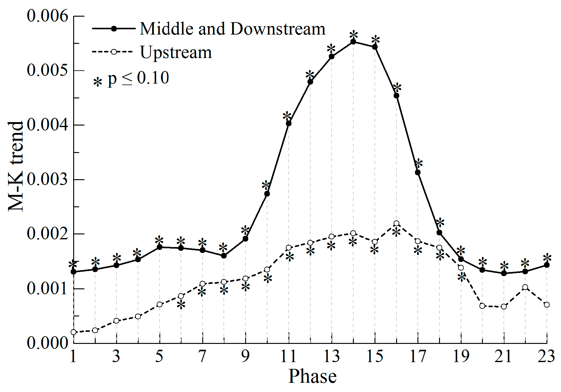
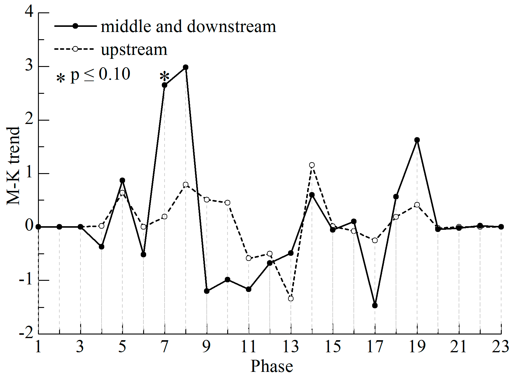
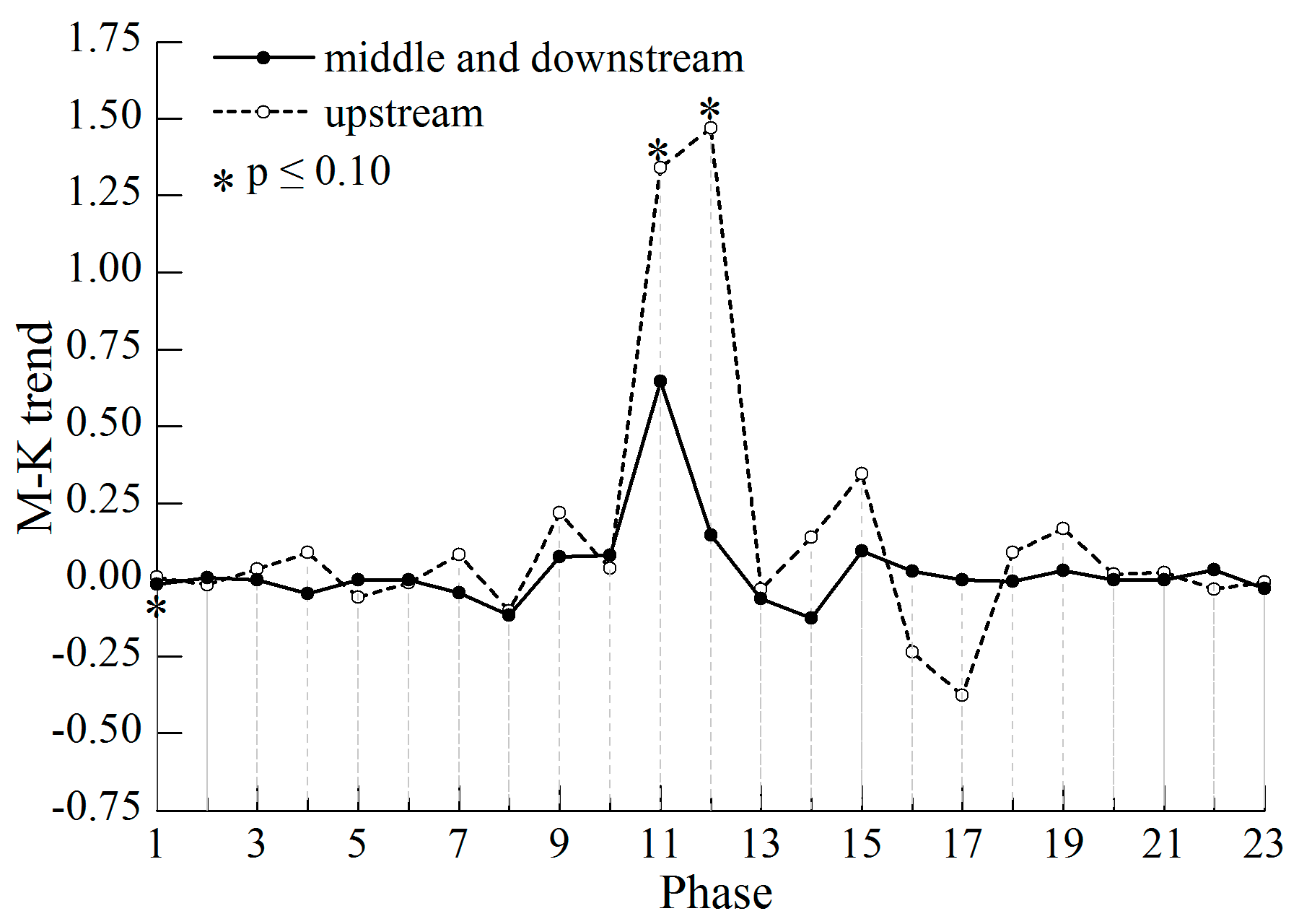
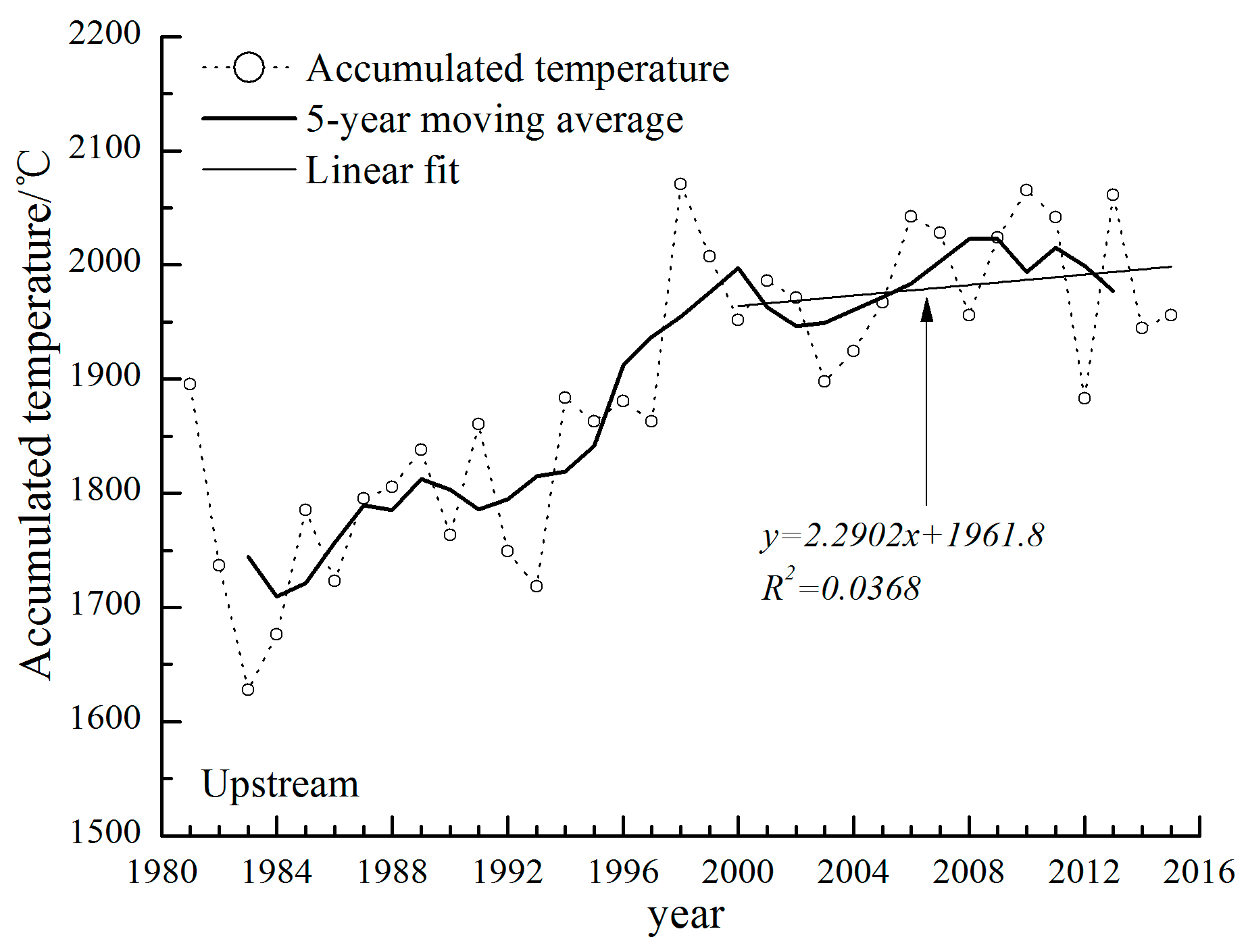
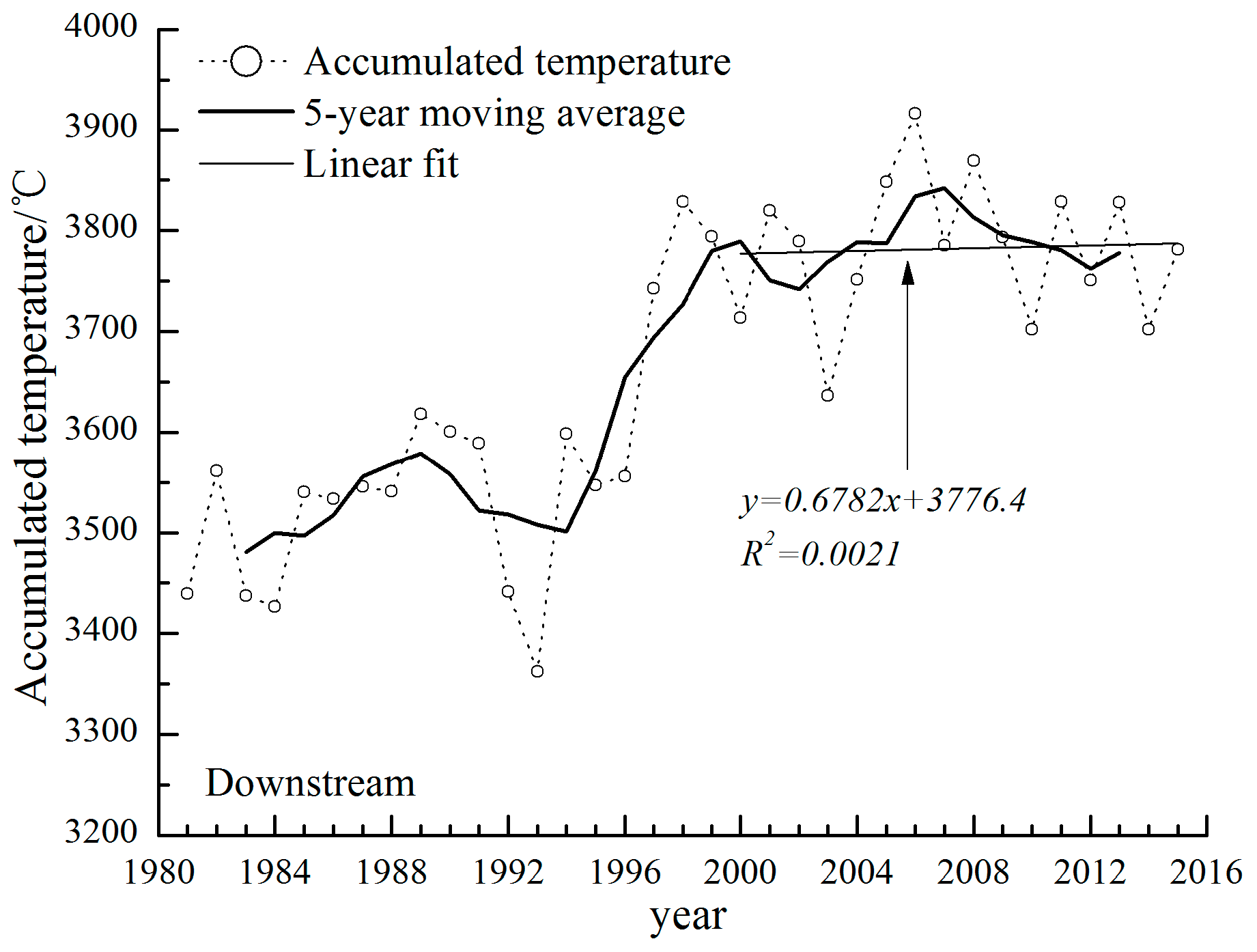
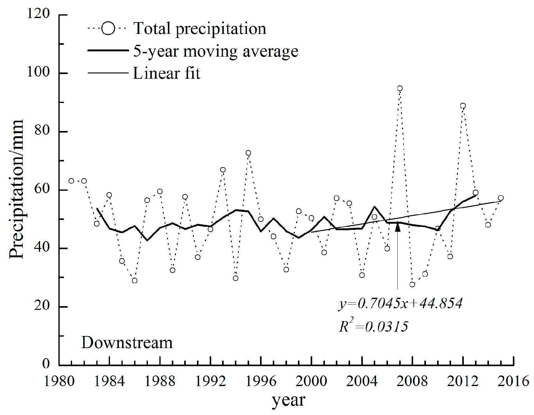
4.3.2. Trends of NDVI and Climatic Factors in a Year

All β values calculated by Equation (6) are positive, which means that NDVI has significantly increased during 2000–2015. In addition, great variations in NDVI mainly appear in the growing seasons (phases 8–20). The variation range in downstream area is much larger than that in upstream area (Figure 7). The increasing trends of total precipitation and accumulated temperature (≥0 °C) are far less obvious than that of NDVI. Their β values are near zero in non-growing season (from phase 20 in current year to phase 6 in the following year), and only a few β values in growing season reach the significance level. The maximum β values of accumulated temperature appear in phases 7 and 8 (6 April to 8 May) in downstream area, which means that increased temperature during vegetation recovery stage has positive impacts on NDVI (Figure 8). Similarly, precipitation is significantly increased in phases 11 and 12 (10 June to 12 July), when vegetation is in vigorous growing period under good hydrothermal conditions. Thus, the increased precipitation is very favorable for plant growth (Figure 9). This is consistent with relevant research, which considered that vegetation growth is mainly controlled by temperature in spring and autumn, and precipitation in summer [30].

4.4. Impact of Climatic Change on NDVI

Results of panel unit root tests show that the time series of four variables (NDVI, precipitation, accumulated temperature, and temperature) are stationary at level value, and all statistics are significant at the 1% level (

Table 5. Panel unit root tests of NDVI and climatic factors (Statistic).

		LLC	Breitung	IPS	Fisher	HT
NDVI	upstream	−8.0570 ***	−6.6448 ***	−5.7781 ***	−8.7002 ***	0.1909 ***
	downstream	−4.4107 ***	−1.5658 **	−2.4993 ***	−2.4852 ***	0.6760 ***
Precipitation	upstream	−5.7606 ***	−9.4949 ***	−9.4238 ***	−5.1822 ***	−0.1524 ***
	downstream	−7.7871 ***	−8.7712 ***	−8.3680 ***	−3.3978 ***	−0.0013 ***
Accumulated temperature	upstream	−6.2357 ***	−7.3473 ***	−7.0134 ***	−6.1442 ***	−0.0515 ***
	downstream	−5.9864 ***	−8.0651 ***	−8.1293 ***	−6.5662 ***	−0.0535 ***
Temperature	upstream	−8.9307 ***	−6.7161 ***	−8.8995 ***	−6.2323 ***	−0.0939 ***
	downstream	−7.4510 ***	−7.9551 ***	−8.6820 ***	−6.8601 ***	−0.1733 ***

Notes: *** p ≤ 0.01.

). Then, we set up panel data models to perform empirical analysis.

4.4.1. The Overall Effect of the Panel Regression Models

Due to the variety of panel data models, we employed 10 different models to estimate explanatory variable parameters: (1) the pooled Ordinary Least Squares (OLS); (2) fixed effects (FE); (3) fixed effects between group (BE); (4) the corrected Least Square Dummy Variables (LSDV); (5) hetonly and two-way fixed effects (FE-TW); (6) Random effects (RE); (7) the feasible generalized least squares (FGLS); (8) Lagrange Multiplier (LM) test for individual-specific effects (MLE); (9) the linear regression with panel-corrected standard errors (PCSE); and (10) two step of Generalized Method of Moment (2S-GMM). The results estimated by Stata 14 are listed in

Table 6. Parameter estimation results of panel data models in upstream area.

No.	Model	Cons	Pre	Atem	R2	χ2	F
1	OLS	0.08029 *** (0.00164)	0.00040 ** (0.00017)	0.00047 *** (0.00002)	0.8096		775.85 ***
2	FE	0.12000 *** (0.00527)	0.00018 (0.00013)	0.00003 (0.00006)	0.8624		1.19
3	BE	0.07961 *** (0.00566)	−0.00012 * (0.00168)	0.00053 ** (0.00020)	0.8697		66.76 ***
4	LSDV	0.07928 *** (0.00313)	0.00018 (0.00014)	0.00004 (0.00005)	0.9447		170.13 ***
5	FE_TW	0.11352 *** (0.00377)	0.00013 (0.00009)	0.00002 (0.00004)	0.8613		3669.19 ***
6	RE	0.09402 *** (0.00472)	0.00030 *** (0.00010)	0.00032 *** (0.00003)	0.8690	115.50 ***
7	FGLS	0.09589 *** (0.00546)	0.00035 ** (0.00016)	0.00029 *** (0.00005)	0.8687	54.28 ***
8	MLE	0.10613 *** (0.00889)	0.00028 *** (0.00011)	0.00018 *** (0.00006)		13.92 ***
9	PCSE	0.08308 *** (0.00283)	0.00025 ** (0.00011)	0.00048 *** (0.00001)	0.8515	217.90 ***
10	2S-GMM	0.11213 *** (0.00060)	0.00028 *** (0.00003)	0.00011 *** (0.000005)	0.8096	446.47 ***

Notes: Standard errors in parentheses. * p ≤ 0.1, ** p ≤ 0.05, *** p ≤ 0.01, the asterisks of coefficients indicate t test.

and

Table 7. Parameter estimation results of panel data models in downstream area.

No.	Model	Cons	Pre	Atem	R2	χ2	F
1	OLS	0.09791 *** (0.00269)	0.00092 * (0.00047)	0.00034 *** (0.00001)	0.6993		424.33 ***
2	FE	0.14486 *** (0.00527)	0.00071 ** (0.00027)	0.00006* (0.00003)	0.7460		7.27 ***
3	BE	0.09870 *** (0.01072)	−0.00182 (0.00732)	0.00037 *** (0.00010)	0.7527		30.44 ***
4	LSDV	0.10211 *** (0.00319)	0.00071 ** (0.00029)	0.00006 (0.00004)	0.9379		175.24 ***
5	FE-TW	0.13509 *** (0.00476)	0.00039** (0.00015)	0.00003 (0.00002)	0.7463		165.24 ***
6	RE	0.128991 *** (0.00724)	0.00069 *** (0.00015)	0.00016 *** (0.00002)	0.7502	55.67 ***
7	FGLS	0.118130 *** (0.00650)	0.00092 *** (0.00030)	0.00022 (0.00003)	0.7503	56.42 ***
8	MLE	0.12105 *** (0.01070)	0.00090 *** (0.00024)	0.00020 *** (0.00004)		24.41 ***
9	PCSE	0.10313 *** (0.00290)	0.00081 *** (0.00016)	0.00022 *** (0.00003)	0.8162	68.87 ***
10	2S-GMM	0.13437 *** (0.00635)	0.00176 *** (0.00017)	0.00008 ** (0.00004)		187.51 ***

Notes: Standard errors in parentheses, * p ≤ 0.1, ** p ≤ 0.05, *** p ≤ 0.01, the asterisks of coefficients indicate t test.

. The values of same parameter in 10 models are very close to each other, and their constant term α changes from 0.0796 to 0.12 in upstream area and from 0.098 to 0.145 in downstream area. The variation in coefficients β among 10 models is also small. Precipitation β ranges from −0.12‰ to 0.4‰ in upstream area and from −1.82‰ to 1.76‰ in downstream area. Temperature β ranges from 0.03‰ to 0.53‰ in upstream area and from 0.03‰ to 0.37‰ in downstream area. The determination coefficients R² greater than 0.8 in upstream area and 0.7 in downstream area, χ² tests and most F tests reach the highly significant level (p ≤ 0.01, Table 6 and Table 7). These indicate that all panel regression models have good robustness.

4.4.2. Contribution of Climatic Change to NDVI

Parameters estimated by the panel regression models could quantify the impacts of change in climatic factors on vegetation growth. All coefficients are positive values (except that of precipitation in BE model) (Table 6 and Table 7), implying that precipitation and accumulated temperature have positive contribution to NDVI. With every 1-mm increase in rainfall, NDVI increases by around 0.223‰ (the mean of ten values) in upstream area and 0.6‰ in downstream area. This illustrates that vegetation growth has stronger responses to rainfall in downstream area with less precipitation than in upstream area with more precipitation. With every 1-°C increase in accumulated temperature, NDVI increases by around 0.241‰ in upstream area and 0.174‰ in downstream area. The coefficients have only small differences between upstream and downstream area. This illustrates that responses of NDVI to accumulated temperature are more moderate.

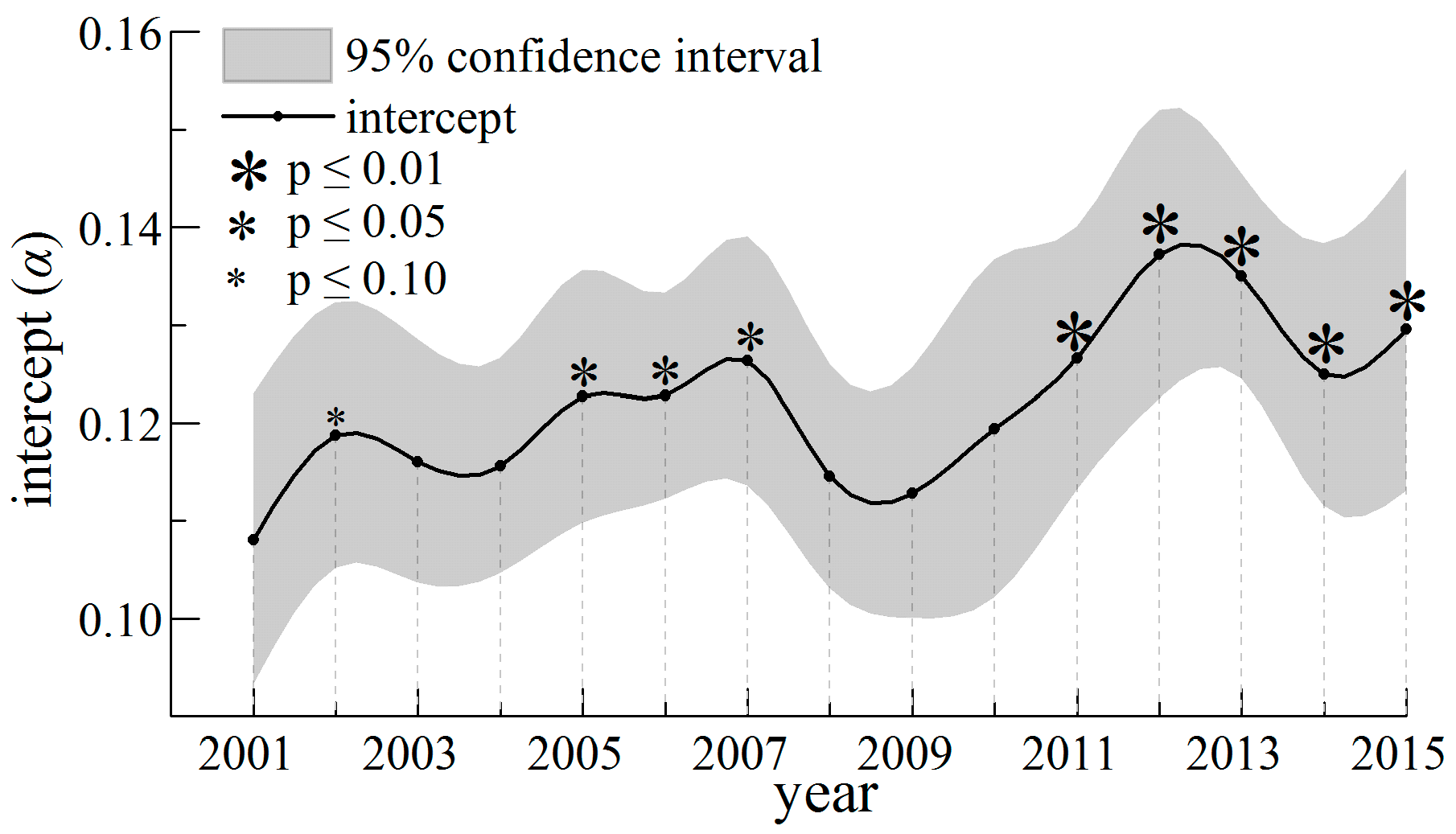
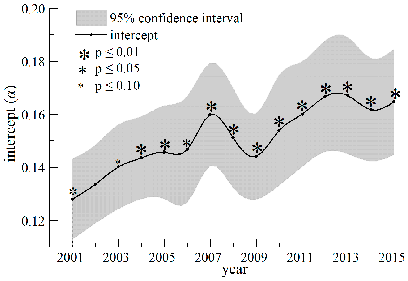
4.4.3. Individual-Specific Effect in Phase and Year

The pooled regression model (OLS) estimates the mixed influence of explanatory variables on dependent variable, but it could not provide information about individual effect and structure change. Individual-specific effect exists in the form of fixed or random effects. FE, BE, LSDV and FE-TW (No. 2–5) belong to the fixed effects model; RE FGLS, MLE and PCSE (No. 6–9) belong to the random effects model; and 2S-GMM is the dynamic panel model as a contrast. Two types of effects appear from intercept items α_i by individual and time. Hausman test indicates that the fixed effect model should be selected in this empirical analysis (

Table 8. Hausman test for the fixed effects and the random effects.

	FE	RE	Difference	Std. Err.
Constant	0.1199954	0.958935	0.0241019	-
Precipitation	0.000175	0.0003507	−0.0001757	0.0000291
Temperature	0.000035	0.000293	−0.0002582	0.0000414

Test (H₀): difference in coefficients is not systematic. χ² = 38.89, p = 0.00.

). However, there are only little differences in parameters estimated by the two types of model, so we mainly focus on the variation of intercept items α_i rather than the type of effect. The results estimated using the variable intercept model show that the individual effects α_i changes with phase, that is, α₁ ≠ α₂, …, ≠ α_N, so we reject the null hypothesis H₁. For instance, FE-TW regression model is expressed as follows:

$$\begin{array}{c}NDV{I}_{it}=\{\begin{array}{l}0.11352(upstream)\\ 0.13509(downstream)\end{array}+{\alpha }_i+\{\begin{array}{l}0.00013(upstream)\\ 0.00039(downstream)\end{array}Pr{e}_{it}+\{\begin{array}{l}0.00002(upstream)\\ 0.00003(downstream)\end{array}Ate{m}_{it}\\ (i=1,2,\cdot \cdot \cdot ,23;t=1,2,\cdot \cdot \cdot ,16)\end{array}$$

α_i begin to rise in about phase 7 (about early April), peak in phase 14 (28 July to 12 August), and then decline, and form an inverted U-shaped curve (Figure 10 and Figure 11). Most of the t tests in growing season are significant at p ≤ 0.05 level. Obviously, α_i (individual effects) seasonally changes, which is consistent with the process of plant growth. In addition, α_i rises over the years (time effects), but the variation is small and most t tests are non-significant (Figure 12 and Figure 13). Thus, the intercept item α_i mainly changes with phase (individual effects are more significant than time effects).

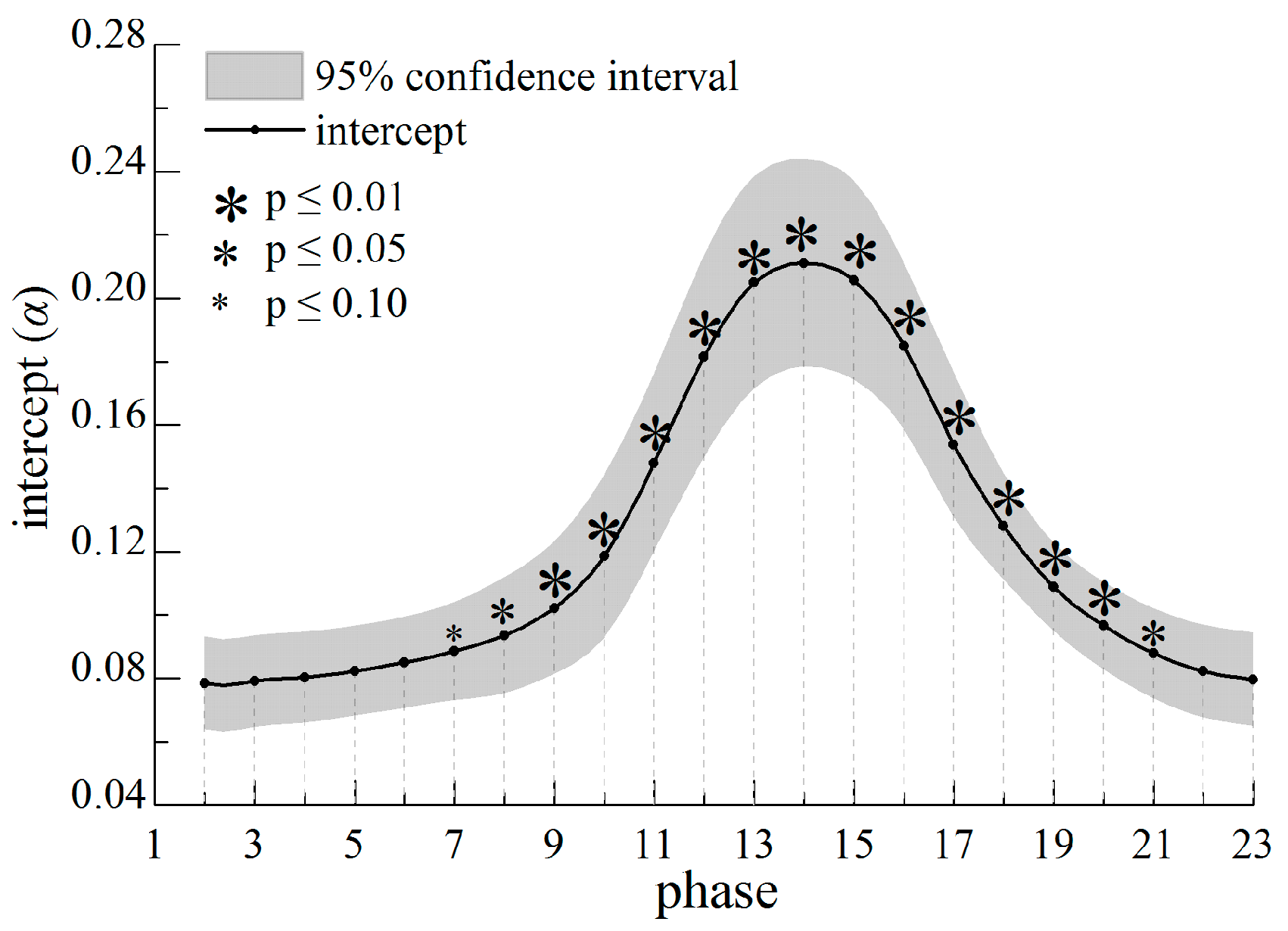
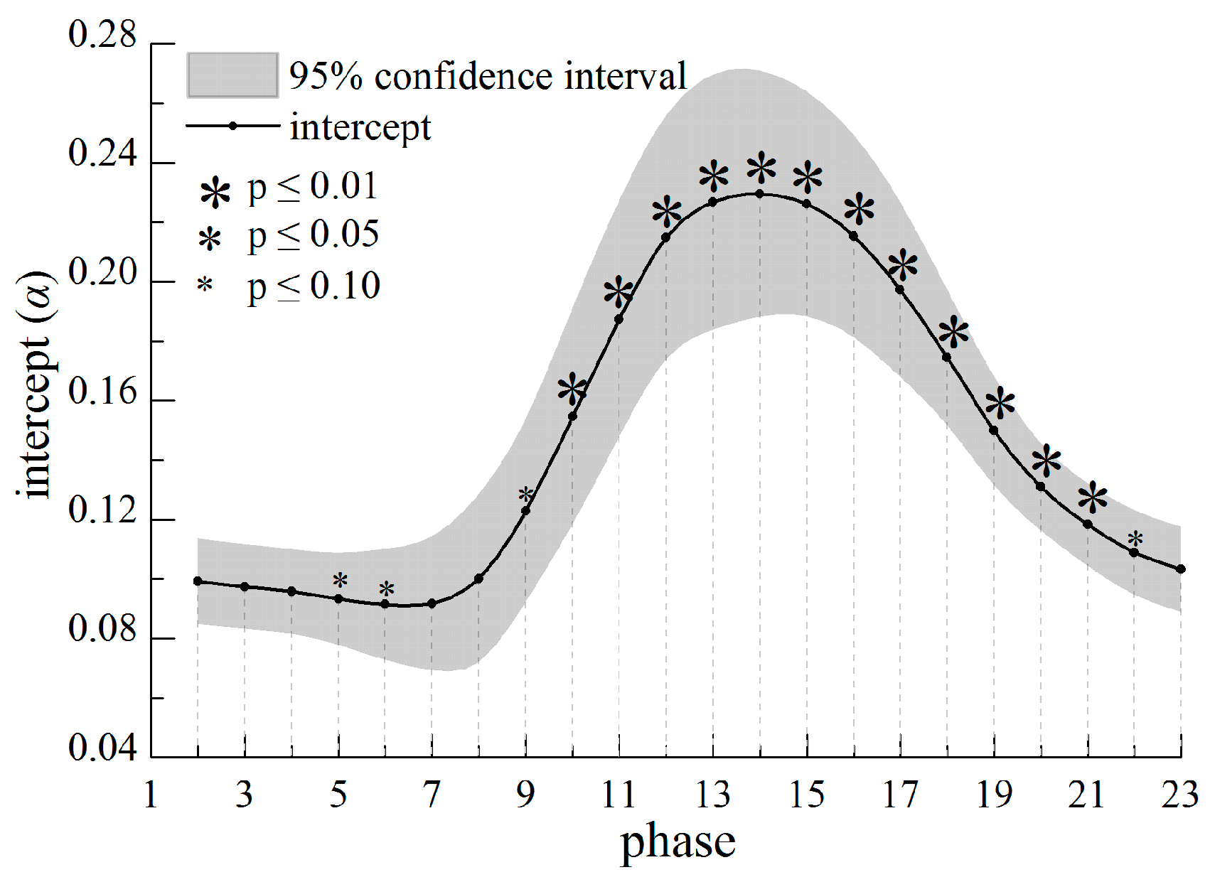
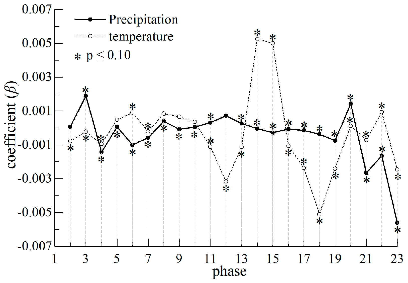
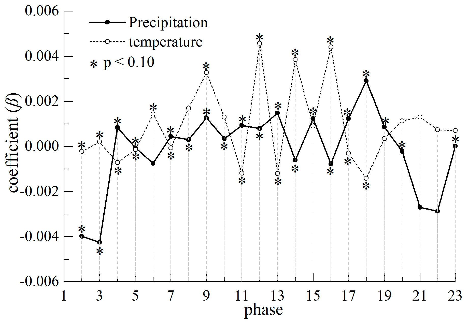
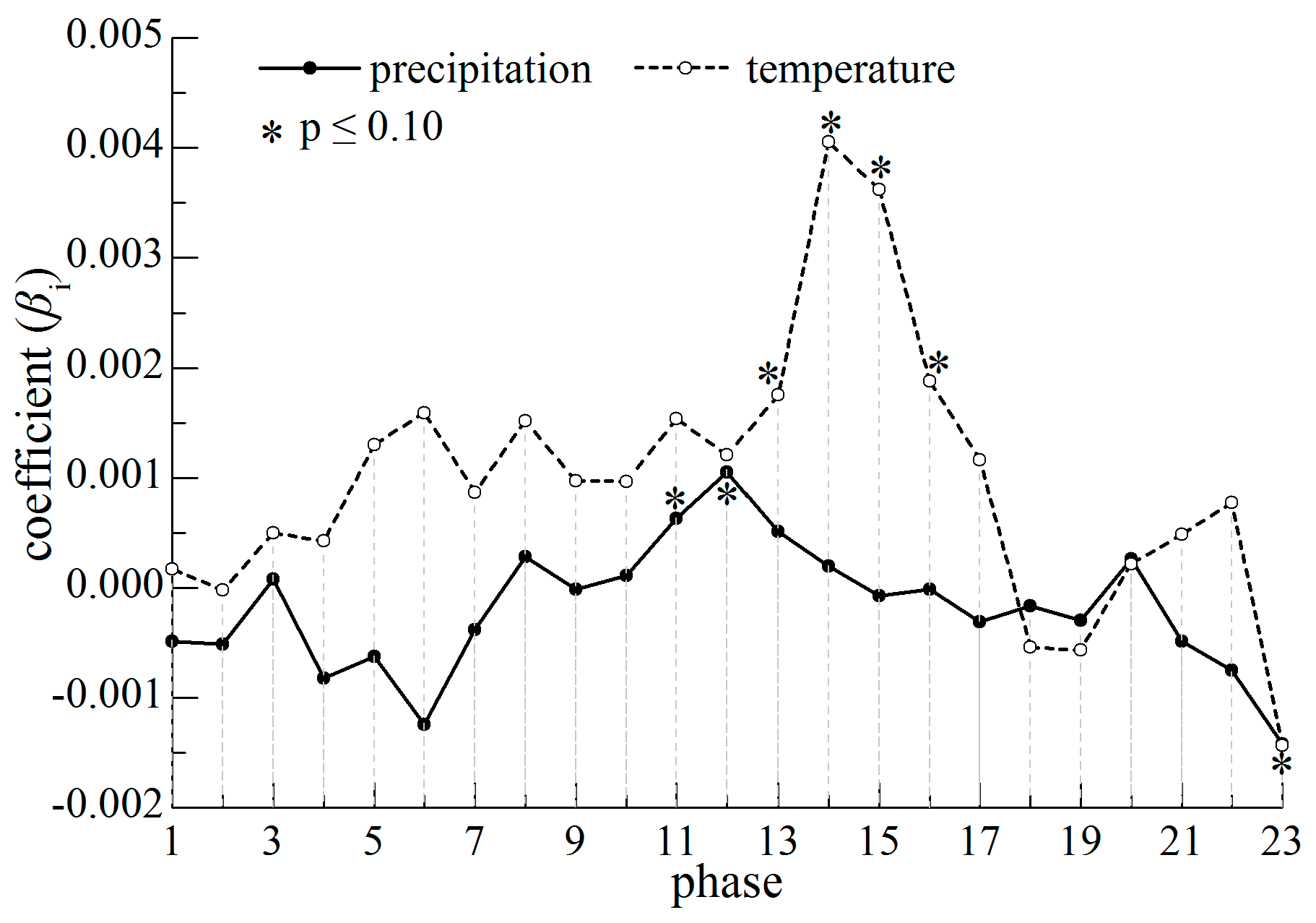
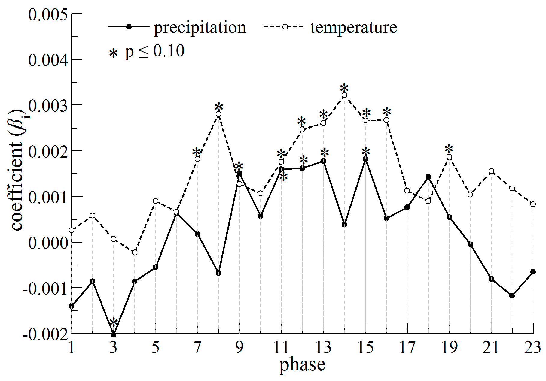
4.4.4. Coefficients Variation with Phase

In order to verify whether and how the coefficient β changes, we employed two variable coefficient models to estimate parameters, one is Dummy Variable-LSDV model (DV-LSDV, introducing dummy variables for phases in LSDV model), the other is the random coefficient model (RC). Interactive items (β) between the dummy variable and the explanatory variables are significant in DV-LSDV (Figure 14 and Figure 15), and most t tests reach very significant level, so the variable coefficient models should be adopted.

β consists of β₀ and β_i in RC models, and β_i is the variable coefficient with phase and year. The estimation results of α_i and β₀ are shown in

Table 9. Parameter estimation results of the random coefficient model.

Region	Constant (αi)	Precipitation (β0)	Temperature (β0)	χ2 (Wald)	χ2 (Test of Parameter Constancy)
Upstream	0.112663 *** (0.011126)	−0.0001927 (0.000469)	0.000979 (0.000687)	2.33	1307.78 ***
Downstream	0.134833 *** (0.012624)	0.000188 0.0005347	0.001483 *** 0.0005626	6.53 **	2454.42 ***

Notes: Standard errors in parentheses, ** p ≤ 0.05, *** p ≤ 0.01, the asterisks of each coefficients indicate t test.

. Although some t tests for β₀ are not statistically significant, χ² tests of parameter constancy reach significance level at p ≤ 0.01. Some t tests for β_i are very significant (Figure 16 and Figure 17). Therefore, we reject the null hypothesis H₂ that coefficient is constant. Unlike variations in intercept term α_i, β variations lack smoothness or regularity, and the process and extent of change are also different among phases and regions.

Therefore, the panel model for vegetation change and climatic factors is both the variable intercept model and variable coefficient model. This is mainly because the individual is phase, which represents different times in a year rather than unit of cross section.

5. Discussion and Conclusions

5.1. Discussion

The global vegetation activity has strengthened during the last 30 years, a trend that is supported by increasing evidence [7,8,9]. Particularly, the greening trend is more attractive in middle and high latitudes of the Northern Hemisphere [7,8,10,11]. The vegetation dynamics in Shule River Basin from 2000 to 2015 precisely reflects the greening trend, which has a better representation in arid and semi-arid regions [4,14]. However, the greening trend has spatial heterogeneity, whereby most of the vegetation improvement areas appear in upstream region adjoining northern Tibetan plateau, because both temperature and precipitation change more significantly in higher altitude area (see Figure 18, Figure 19, Figure 20 and Figure 21). The more evident greening trend shows around newly developed fields in downstream area, which is the result influenced by agriculture irrigation.

It is known that global warming has accelerated [8]. This situation has a typical performance in Shule River Basin, i.e., the accumulated temperature remains at a higher level during growing season since 2000, as shown in Figure 18 and Figure 19. Especially, the linear growth rate of the accumulated temperature in upstream reached 2.29 °C/year (see Figure 18). The total precipitation during growing season also shows an increasing tendency in Shule River Basin (Figure 20 and Figure 21), especially the upstream has a strong performance with a linear growth rate of 2.36 mm/year (see Figure 20). Recent research by Wang et al. indicated that the runoff from mountainous areas in Shule River Basin increased significantly during the past 50 years [56], which reflects the climatic change trend. Therefore, we attribute the vegetation variation to precipitation and temperature increasing in Shule River Basin, which is consistent with other results [57].

The most important finding of this paper is that responses of vegetation variation to the climatic factors that are more scarce more sensitive in Shule River Basin, and marginal contributions of climatic factors change are calculated, which benefits by applying panel data models. Though precipitation and accumulated temperature have positive contributions to NDVI, their impacts are different in upstream and downstream areas. The impact of precipitation on NDVI is larger in the more arid downstream area than in upstream area, whereas the effect of temperature is larger in the cooler upstream area than in downstream area.

In addition to precipitation and temperature, some other factors also influence plant growth, such as wind speed, humidity, human activities, and so on. Unfortunately, there is a lack of time series data for these indexes. Moreover, it is difficult to confirm the impacts of social and economic activities on vegetation growth in different phases. In our study, the impact of human activities on plant growth in upstream mountain is insignificant compared to that in downstream plain. The differences in vegetation variation during 2000–2015 between upstream and downstream areas are caused by both natural geographical conditions and human activities, and the vegetation improvement around resettlement places are more likely the result of irrigation expansion. Even so, precipitation and temperature are still the two basic factors influencing vegetation growth, and our results are meaningful for grassland ecological protection in Shule River Basin.

The panel data model is a very powerful tool to process massive data in three dimensions from variable, time series and cross section. We employed this model to analyze the impact of climatic factors on NDVI in Shule River Basin. It should be emphasized that we replace cross section of individuals with phases and investigated the trend and characteristics of vegetation variation over phases and years. The results estimated by panel data models provide some useful information that other methods cannot provide. For instance, the contribution of unit precipitation and temperature to NDVI in different phases is obtained, intercept α changes with phases and the curve of it has inverted U-shape, responses of vegetation growth to climatic factors are more sensitive when these factors are limiting than when they are not. Since there is only 16-year NDVI data, it is difficult to fully display the influence of climate change on NDVI. If longer time series are available, the panel data model will give better results.

Vegetation coverage has been in a continuously greening trend in Shule River Basin, but it does not fundamentally alter the situation of ecological fragility in this region. The vegetation degradation appears mostly in downstream area where there are more human activities. For local region, it is difficult to control climate change to protect the environment. Thus, limiting large-scale use of water and land resources and mitigating human impacts on environment might be the best way to protect environment.

5.2. Conclusions

During 2000–2015, the vegetation has been in an obvious greening trend in Shule River Basin in northwest China, which is in response to climate change. The greening areas, i.e., areas with vegetation improvement, account for 92.70% of the whole basin. Moreover, upstream mountain has larger greening areas than downstream plain. Vegetation degradation appears in downstream region, and the vegetation type mainly includes meadow halophytes.

The multiple correlations between NDVI and climatic factors show that the response of vegetation to climate change significantly lags. Current vegetation growth depends largely on the climate condition half to one month ago. The M-K trend detection shows that vegetation growth is mainly influenced by temperature in spring and autumn and precipitation in summer.

Then, we employed a set of panel data models to estimate the impacts of climatic factors on NDVI in Shule river basin. The results provide some useful information on change in vegetation coverage: (1) All panel regression models have good robustness, the constant term α and coefficients β have only little variation between different models, and most parameters estimated are statistically significant. (2) NDVI increases with increase in precipitation and temperature in Shule River Basin. With every 1-mm increase in precipitation, NDVI increases by 0.223‰ in upstream area and 0.6‰ in downstream area. With every 1-°C increase in accumulated temperature, NDVI increases by around 0.241‰ in upstream area and 0.174‰ in downstream area. The effect of precipitation is larger in the more arid downstream area than in upstream area, whereas the effect of temperature is larger in the cooler upstream area than in downstream area. This illustrates that responses of NDVI to climatic factors are more sensitive when these factors are limiting than when these factors are not limiting. (3) The variable intercept model shows that the intercept α_i first increases and then decreases over the phases, and forms an inverted U-shaped curve. This reflects the seasonal characteristics of vegetation growth. In addition, intercept α_i increases over the years (time effect), indicating a vegetation greening trend, though this effect is much weaker than the individual effect. Thus, we reject the null hypothesis H₁ that assumes α₁ = α₂ = … = α_N. (4) The variable coefficient models show that β_i changes over phases, so we reject the null hypothesis H₂ that assumes β₁ = β₂, … = β_N. The variations in coefficients lack smoothness or regularity, which is different from variations in intercept α_i. In summary, the panel data models for NDVI and two climatic factors are both the variable intercept models and the variable coefficient models, representing features of vegetation variations in Shule River Basin.

References

1. De Jong, R.; de Bruin, S.; de Wit, A.; Schaepman, M.E.; Dent, D.L. Analysis of monotonic greening and browning trends from global NDVI time-series. Remote Sens. Environ. 2011, 115, 692–702. [Google Scholar] [CrossRef] [Green Version]
2. Parmesan, C.; Yohe, G. A globally coherent fingerprint of climate change impacts across natural systems. Nature 2003, 421, 37–42. [Google Scholar] [CrossRef] [PubMed]
3. Du, J.; Zhao, C.; Shu, J.; Jiaerheng, A.; Yuan, X.; Yin, J.; Fang, S.; He, P. Spatiotemporal changes of vegetation on the Tibetan Plateau and relationship to climatic variables during multiyear periods from 1982–2012. Environ. Earth Sci. 2016, 75, 1–18. [Google Scholar] [CrossRef]
4. Fensholt, R.; Langanke, T.; Rasmussen, K.; Reenberg, A.; Prince, S.D.; Tucker, C.; Scholes, R.J.; Le, Q.B.; Bondeau, A.; Eastman, R.; et al. Greenness in semi-arid areas across the globe 1981–2007—An Earth Observing Satellite based analysis of trends and drivers. Remote Sens. Environ. 2012, 121, 144–158. [Google Scholar] [CrossRef]
5. Tucker, C.J.; Newcomb, W.W.; Los, S.O.; Prince, S.D. Mean and inter-year variation of growing-season normalized difference vegetation index for the Sahel 1981–1989. Int. J. Remote Sens. 1991, 12, 1133–1135. [Google Scholar] [CrossRef]
6. Myneni, R.B.; Hall, F.G. The interpretation of spectral vegetation indexes. IEEE Trans. Geosci. Remote. Sens. 1995, 33, 481–486. [Google Scholar] [CrossRef]
7. Liu, Y.; Li, Y.; Li, S.; Motesharrei, S. Spatial and Temporal Patterns of Global NDVI Trends: Correlations with Climate and Human Factors. Remote Sens. 2015, 7, 13233–13250. [Google Scholar] [CrossRef]
8. Wu, D.; Wu, H.; Zhao, X.; Zhou, T.; Tang, B.; Zhao, W.; Jia, K. Evaluation of Spatiotemporal Variations of Global Fractional Vegetation Cover Based on GIMMS NDVI Data from 1982 to 2011. Remote Sens. 2014, 6, 4217–4239. [Google Scholar] [CrossRef]
9. De Jong, R.; Schaepman, M.E.; Furrer, R.; De Bruin, S.; Verburg, P.H. Spatial relationship between climatologies and changes in global vegetation activity. Glob. Chang. Biol. 2013, 19, 1953–1964. [Google Scholar] [CrossRef] [PubMed]
10. Mao, J.; Shi, X.; Thornton, P.E.; Hoffman, F.M.; Zhu, Z.; Myneni, R.B. Global Latitudinal-Asymmetric Vegetation Growth Trends and Their Driving Mechanisms: 1982–2009. Remote Sens. 2013, 5, 1484–1497. [Google Scholar] [CrossRef]
11. Sobrino, J.A.; Julien, Y. Global trends in NDVI-derived parameters obtained from GIMMS data. Int. J. Remote Sens. 2011, 32, 4267–4279. [Google Scholar] [CrossRef]
12. Wang, X.; Piao, S.; Ciais, P.; Li, J.; Friedlingstein, P.; Koven, C.; Chen, A. Spring Temperature Change and Its Implication in the Change of Vegetation Growth in North America From 1982 to 2006. Proc. Natl. Acad. Sci. USA 2011, 108, 1240–1245. [Google Scholar] [CrossRef] [PubMed]
13. Zhao, M.; Running, S.W. Drought-induced reduction in global terrestrial net primary production from 2000 through 2009. Science 2010, 329, 940–943. [Google Scholar] [CrossRef] [PubMed]
14. Vicente-Serrano, S.M.; Cabello, D.; Tomás-burguera, M.; Martín-Hernández, N.; Beguería, S.; Azorin-Molina, C.; Kenawy, A.E. Drought Variability and Land Degradation in Semiarid Regions: Assessment Using Remote Sensing Data and Drought Indices (1982–2011). Remote Sens. 2015, 7, 4391–4423. [Google Scholar] [CrossRef]
15. Gang, Y.; Hu, Z.; Chen, X.; Tashpolat, T. Vegetation dynamics and its response to climate change in Central Asia. J. Arid Land 2016, 8, 375–388. [Google Scholar]
16. Li, Z.; Chen, Y.; Li, W.; Deng, H.; Fang, G. Potential impacts of climate change on vegetation dynamics in Central Asia. J. Geophys. Res. Atmos. 2015, 120, 2045–2057. [Google Scholar] [CrossRef]
17. Mohammat, A.; Wang, X.; Xu, X.; Peng, L.; Yang, Y.; Zhang, X.; Mynenic, R.B.; Piao, S. Drought and spring cooling induced recent decrease in vegetation growth in Inner Asia. Agric. For. Meteorol. 2013, 178–179, 21–30. [Google Scholar] [CrossRef]
18. Piao, S.; Wang, X.; Ciais, P.; Zhu, B.; Wang, T.; Liu, J. Changes in satellite-derived vegetation growth trend in temperate and boreal Eurasia from 1982 to 2006. Glob. Chang. Biol. 2011, 17, 3228–3239. [Google Scholar] [CrossRef]
19. Dardel, C.; Kergoat, L.; Hiernaux, P.; Mougin, E.; Grippa, M.; Tucker, C.J. Re-greening Sahel: 30 years of remote sensing data and field observations (Mali, Niger). Remote Sens. Environ. 2014, 140, 350–364. [Google Scholar] [CrossRef]
20. Donohue, R.J.; Mcvicar, T.R.; Roderick, M.L. Climate-related trends in Australian vegetation cover as inferred from satellite observations, 1981–2006. Glob. Chang. Biol. 2009, 15, 1025–1039. [Google Scholar] [CrossRef]
21. Zhang, L.; Guo, H.; Wang, C.; Ji, L.; Li, J.; Wang, K.; Dai, L. The long-term trends (1982–2006) in vegetation greenness of the alpine ecosystem in the Qinghai-Tibetan Plateau. Environ. Earth Sci. 2014, 72, 1827–1841. [Google Scholar] [CrossRef]
22. Sun, J.; Qin, X. Precipitation and temperature regulate the seasonal changes of NDVI across the Tibetan Plateau. Environ. Earth Sci. 2016, 75, 1–9. [Google Scholar] [CrossRef]
23. Zhang, Y.; Peng, C.; Li, W.; Tian, L.; Zhu, Q.; Chen, H.; Fang, X.; Zhang, G.; Liu, G.; Mu, X.; et al. Multiple afforestation programs accelerate the greenness in the ‘Three North’ region of China from 1982 to 2013. Ecol. Indic. 2016, 61, 404–412. [Google Scholar] [CrossRef]
24. Yuan, X.; Li, L.; Chen, X.; Shi, H. Effects of Precipitation Intensity and Temperature on NDVI-Based Grass Change over Northern China during the Period from 1982 to 2011. Remote Sens. 2015, 7, 10164–10183. [Google Scholar] [CrossRef]
25. He, B.; Chen, A.; Wang, H.; Wang, Q. Dynamic Response of Satellite-Derived Vegetation Growth to Climate Change in the Three North Shelter Forest Region in China. Remote Sens. 2015, 7, 9998–10016. [Google Scholar] [CrossRef]
26. Liu, S.; Gong, P. Change of surface cover greenness in China between 2000 and 2010. Chin. Sci. Bull. 2012, 57, 2835–2845. [Google Scholar] [CrossRef]
27. Shen, Z.; Fu, G.; Yu, C.; Sun, W.; Zhang, X. Relationship between the Growing Season Maximum Enhanced Vegetation Index and Climatic Factors on the Tibetan Plateau. Remote Sens. 2014, 6, 6765–6789. [Google Scholar] [CrossRef]
28. Xiao, J.; Zhou, Y.; Zhang, L. Contributions of natural and human factors to increases in vegetation productivity in China. Ecosphere 2015, 6, 1–20. [Google Scholar] [CrossRef]
29. Li, H.; Li, Y.; Gao, Y.; Zou, C.; Yan, S.; Gao, J. Human Impact on Vegetation Dynamics around Lhasa, Southern Tibetan Plateau, China. Sustainability 2016, 8, 1146. [Google Scholar] [CrossRef]
30. Liang, W.; Yang, Y.; Fan, D.; Guan, H.; Zhang, T.; Long, D.; Zhou, Y.; Bai, D. Analysis of spatial and temporal patterns of net primary production and their climate controls in China from 1982 to 2010. Agric. For. Meteorol. 2015, 204, 22–36. [Google Scholar] [CrossRef]
31. Peng, S.; Chen, A.; Xu, L.; Cao, C.; Fang, J.; Myneni, R.B.; Pinzon, J.E.; Tucker, C.J.; Piao, S. Recent change of vegetation growth trend in China. Environ. Res. Lett. 2011, 6, 44027–44039. [Google Scholar] [CrossRef]
32. Xu, G.; Zhang, H.; Chen, B.; Zhang, H.; Innes, J.L.; Wang, G.; Yan, J.; Zheng, Y.; Zhu, Z.; Myneni, R.B. Changes in Vegetation Growth Dynamics and Relations with Climate over China’s Landmass from 1982 to 2011. Remote Sens. 2014, 6, 3263–3283. [Google Scholar] [CrossRef]
33. Liu, Y.; Lei, H. Responses of Natural Vegetation Dynamics to Climate Drivers in China from 1982 to 2011. Remote Sens. 2015, 7, 10243–10268. [Google Scholar] [CrossRef]
34. Zhou, L.; Tucker, C.J.; Kaufmann, R.K.; Slayback, D.; Shabanov, N.V.; Myneni, R.B. Variations in northern vegetation activity inferred from satellite data of vegetation index during 1981 to 1999. J. Geophys. Res. Atmos. 2001, 106, 20069–20084. [Google Scholar] [CrossRef]
35. Nemani, R.R.; Keeling, C.D.; Hashimoto, H.; Jolly, W.M.; Piper, S.C.; Tucker, C.J.; Myneni, R.B.; Running, S.W. Climate-Driven Increases in Global Terrestrial Net Primary Production from 1982 to 1999. Science 2003, 300, 1560–1563. [Google Scholar] [CrossRef] [PubMed]
36. Herrmann, S.M.; Anyamba, A.; Tucker, C.J. Recent trends in vegetation dynamics in the African Sahel and their relationship to climate. Glob. Environ. Chang.-Hum. 2005, 15, 394–404. [Google Scholar] [CrossRef]
37. Liu, L.; Zhao, X.; Chang, X.; Lian, J. Impact of Precipitation Fluctuation on Desert-Grassland ANPP. Sustainability 2016, 8, 1245. [Google Scholar] [CrossRef]
38. Duan, H.; Yan, C.; Tsunekawa, A.; Song, X.; Li, S.; Xie, J. Assessing vegetation dynamics in the Three-North Shelter Forest region of China using AVHRR NDVI data. Environ. Earth Sci. 2011, 64, 1011–1020. [Google Scholar] [CrossRef]
39. Han, K.S.; Park, Y.Y.; Yeom, J.M. Detection of change in vegetation in the surrounding Desert areas of Northwest China and Mongolia with multi-temporal satellite images. Asia-Pacific. J. Atmos. Sci. 2015, 51, 173–181. [Google Scholar]
40. Lu, Y.; Zhang, L.; Feng, X.; Zeng, Y.; Fu, B.; Yao, X.; Li, J.; Wu, B. Recent Ecological Transitions in China: Greening, Browning, and Influential Factors. Sci. Rep. 2015, 5, 8732. [Google Scholar] [CrossRef] [PubMed]
41. Yang, X.; Liu, S.; Yang, T.; Xu, X.; Kang, C.; Tang, J.; Wei, H.; Ghebrezgabher, M.G.; Li, Z. Spatial-temporal dynamics of desert vegetation and its responses to climatic variations over the last three decades: A case study of Hexi region in Northwest China. J. Arid Land 2016, 8, 556–568. [Google Scholar] [CrossRef]
42. Wang, H.; Liu, G.; Li, Z.; Ye, X.; Wang, M.; Gong, L. Impacts of climate change on net primary productivity in arid and semiarid regions of China. Chin. Geogr. Sci. 2016, 26, 35–47. [Google Scholar] [CrossRef]
43. De Jong, R.; Verbesselt, J.; Schaepman, M.E.; de Bruin, S. Trend changes in global greening and browning: Contribution of short-term trends to longer-term change. Glob. Chang. Biol. 2012, 18, 642–655. [Google Scholar] [CrossRef]
44. Cihlar, J.; Ly, H.; Li, Z.; Chen, J.; Pokrant, H.; Huang, F. Multitemporal, multichannel AVHRR data sets for land biosphere studies—Artifacts and corrections. Remote Sens. Environ. 1997, 60, 35–57. [Google Scholar] [CrossRef]
45. Jönsson, P.; Eklundh, L. TIMESAT—A program for analyzing time-series of satellite sensor data. Comput. Geosci. 2004, 30, 833–845. [Google Scholar] [CrossRef]
46. Ding, M.; Zhang, Y.; Sun, X.; Liu, L.; Wang, Z.; Bai, W. Spatiotemporal variation in alpine grassland phenology in the Qinghai-Tibetan Plateau from 1999 to 2009. Chin. Sci. Bull. 2013, 58, 396–405. [Google Scholar] [CrossRef]
47. Ma, M.; Frank, V. Interannual Variability of Vegetation Cover in the Chinese Heihe River Basin and Its Relation to Meteorological Parameters. Int. J. Remote Sens. 2006, 27, 3473–3486. [Google Scholar] [CrossRef]
48. Song, Y.; Ma, M. A statistical analysis of the relationship between climatic factors and the Normalized Difference Vegetation Index in China. Int. J. Remote Sens. 2011, 45, 374–382. [Google Scholar] [CrossRef]
49. Yue, S.; Pilon, P.; Phinney, B.; Cavadias, G. The influence of autocorrelation on the ability to detect trend in hydrological series. Hydrol. Process. 2002, 16, 1807–1829. [Google Scholar] [CrossRef]
50. Yue, S.; Wang, C. The Mann-Kendall Test Modified by Effective Sample Size to Detect Trend in Serially Correlated Hydrological Series. Water Resour. Manag. 2004, 18, 201–218. [Google Scholar] [CrossRef]
51. Gocic, M.; Trajkovic, S. Analysis of changes in meteorological variables using Mann-Kendall and Sen’s slope estimator statistical tests in Serbia. Glob. Planet. Chang. 2013, 100, 172–182. [Google Scholar] [CrossRef]
52. Hsiao, C. Analysis of Panel Data, 2nd ed.; Cambridge University Press: New York, NY, USA, 2003; pp. 1–10. [Google Scholar]
53. Mahadevan, R.; Asafu-Adjaye, J. Energy consumption, economic growth and prices: A reassessment using panel VECM for developed and developing countries. Energy Policy 2007, 35, 2481–2490. [Google Scholar] [CrossRef]
54. Xu, W.; Liu, X. Response of Vegetation in the Qinghai-Tibet Plateau to Global Warming. Chin. Geogr. Sci. 2007, 17, 151–159. [Google Scholar] [CrossRef]
55. Wu, D.; Zhao, X.; Liang, S.; Zhou, T.; Huang, K.; Tang, B.; Zhao, W. Time-lag effects of global vegetation responses to climate change. Glob. Chang. Biol. 2015, 21, 3520–3531. [Google Scholar] [CrossRef] [PubMed]
56. Wang, H.; Chen, Y.; Li, W.; Deng, H. Runoff Responses to Climate Change in Arid Region of Northwestern China during 1960–2010. Chin. Geogr. Sci. 2013, 23, 286–300. [Google Scholar] [CrossRef]
57. Deng, S.; Yang, T.; Zeng, B. Vegetation Cover Variation in the Qilian Mountains and its Response to Climate Change in 2000–2011. J. Mt. Sci. 2013, 10, 1050–1062. [Google Scholar] [CrossRef]
Figure 1. Location map of Shule River Basin.
Sustainability 09 00368 g001
Figure 2. Intra-annual variations of the average Normalized Difference Vegetation Index (NDVI) in Shule River Basin.
Sustainability 09 00368 g002
Figure 3. Inter-annual variations of average NDVI during growing season (NDVIgs) in Shule River Basin.
Sustainability 09 00368 g003
Figure 4. Spatial distribution of NDVIgs trends in Shule River Basin.
Sustainability 09 00368 g004
Figure 5. Land use/cover map of Shule River Basin in 2007.
Sustainability 09 00368 g005
Figure 6. Microscopic analysis of vegetation variation in typical regions: Region A with positive trend in vegetation (A1A3) and Region B with negative trend in vegetation (B1B3).
Sustainability 09 00368 g006
Figure 7. The trend of NDVI in a year.
Sustainability 09 00368 g007
Figure 8. The trend of accumulated temperature in a year.
Sustainability 09 00368 g008
Figure 9. The trend of precipitation in a year.
Sustainability 09 00368 g009
Figure 10. Intercept variation with phase in upstream area.
Sustainability 09 00368 g010
Figure 11. Intercept variation with phase in downstream area.
Sustainability 09 00368 g011
Figure 12. Intercept variation with year in upstream area.
Sustainability 09 00368 g012
Figure 13. Intercept variation with year in downstream area.
Sustainability 09 00368 g013
Figure 14. Interactive item variation with phase in upstream area.
Sustainability 09 00368 g014
Figure 15. Interactive item variation with phase in downstream area.
Sustainability 09 00368 g015
Figure 16. Coefficient variation with phases in upstream area.
Sustainability 09 00368 g016
Figure 17. Coefficient variation with phases in downstream area.
Sustainability 09 00368 g017
Figure 18. The variation of accumulated temperature during growing season in upstream area.
Sustainability 09 00368 g018
Figure 19. The variation of accumulated temperature during growing season in downstream area.
Sustainability 09 00368 g019
Figure 20. The variation of precipitation during growing season in upstream area.
Sustainability 09 00368 g020
Figure 21. The variation of precipitation during growing season in downstream area.
Sustainability 09 00368 g021