Article

Exploring Change in China’s Carbon Intensity: A Decomposition Approach

1
Center for Economic Research, Shandong University, Jinan 250100, China
2
Collaborative Innovation Center for Energy Economics and Energy Policy, China Institute for Studies in Energy Policy, School of Management, Xiamen University, Xiamen 361005, China
3
Birmingham Centre for Energy Storage, School of Chemical Engineering, University of Birmingham, Edgbaston, Birmingham B15 2TT, UK
*
Author to whom correspondence should be addressed.
Sustainability 2017, 9(2), 296; https://doi.org/10.3390/su9020296
Submission received: 30 December 2016 / Revised: 14 February 2017 / Accepted: 15 February 2017 / Published: 18 February 2017
(This article belongs to the Section Environmental Sustainability and Applications)

Abstract

:
This paper aims to explore the change of CO2 intensity in China at both national and provincial levels. To serve this purpose, we introduce a decomposition model which integrates the merits of index decomposition analysis and production-theoretical decomposition analysis. Based on the decomposition, we also estimate the potential reduction of CO2 intensity for China and its provinces. Using a panel data set including China’s 30 provinces during the period of 2006–2012, the empirical analysis is conducted and meaningful results are obtained. First, the potential energy intensity change was the dominant driving factor for the decrease of CO2 intensity, which contributed to a total reduction of 19.8%. Second, the energy efficiency change and the CO2 emission factor change also play positive roles in the CO2 intensity reduction for most provinces. Third, provinces in the western area generally showed a relatively large potential reduction in CO2 intensity, while those in the eastern area only demonstrated a small reduction.

1. Introduction

Global warming has increasingly attracted attention worldwide and has become a serious challenge for human society. As the major component of greenhouse gas, the increase in CO2 emissions is of particular concern. According to the International Energy Agency (IEA), the global CO2 emissions reached 31.7 Gt CO2 in 2012, and China is the largest contributor, accounting for 26% of the world’s total emissions. Consequently, global CO2 emission mitigation requires a commitment from China to control and reduce emissions from all sources, especially that from fossil fuels. If this does not occur, global CO2 emissions are expected to increase at an even faster rate, due to the contribution of China. Therefore, understanding the features of China’s CO2 emissions is of vital importance. There is a large body of studies analyzing the factors which are influencing China’s CO2 emission. See, for example [1,2,3,4,5,6].
Unlike developed countries, China creates its emissions reduction target using CO2 intensity (defined as CO2 emissions per GDP) as an important indicator. For instance, in 2009, China made a commitment to reduce its CO2 intensity by 40%–45% from 2005 to 2020. In the “Twelfth Five-Year Plan” (2011–2015), the CO2 intensity is scheduled to be reduced by 17%, compared to the 2010 level. An increasing number of studies are placing an emphasis on investigating the driving force of change in China’s CO2 intensity. Representative studies include [7,8,9,10,11].
China is a large country with enormous provincial variations in resource endowments and economic development. Accordingly, there are also large provincial diversities in the change of CO2 intensity. Therefore, China’s emissions reduction targets are usually decomposed at a regional level and assigned to each of its provinces. Thus, a lack of accountability for reduction efforts at the provincial level may lead to a poor implementation of national policy [12]. As a result, tracking the change in China’s CO2 intensity at both a national and provincial level is particularly important for policy makers. However, as far as we know, very few studies have paid attention to the variations of CO2 intensity change across China’s provinces. For example, Zhang et al. [13] employed the LMDI method to explore the driving factors of carbon intensity in China’s 29 Chinese provinces, from 1995 to 2012. Furthermore, Xu et al. [14] analyzed the regional contributions to the national carbon intensity in China in different Five-Year Plan periods. The purpose of this paper is to explore the driving forces of China’s CO2 intensity change at the provincial level, as well as at the national level, using a newly developed decomposition method. Specifically, we decompose the carbon intensity change into six predefined components for each province, respectively. For the purpose of empirical study, we analyze the carbon intensity change for China’s 30 provinces between 2006 and 2012. This can help us gain a deeper understanding of the carbon intensity change at China’s provincial level, through exploring the different driving forces. Similarly, we attribute the change in the carbon intensity of China as a whole into seven predefined effects. We empirically investigate China’s carbon intensity change on a year-by-year basis. In summary, for the analysis of the nation, we explore the time-serial features. However, for the provinces, we focus on the cross-sectional features.
Technically, the driving factors of CO2 intensity change can be analyzed by attributing them to several pre-defined effects, using decomposition analysis. In this context, index decomposition analysis (IDA) has become a popular analytical tool. Xu and Ang [15] provided a comprehensive literature review on applying IDA to CO2 emission studies. Ang [16] compared various IDA methods and concluded that the Logarithmic Mean Divisia Index (LMDI) method was preferable, as it possesses all of the three desirable properties: factor-reversal, time-reversal, and zero-value robust [17]. Currently, the LMDI method is widely used in energy and environmental studies. Despite its strengths, some fundamental factors, such as technical efficiency change and technological change, which play critical roles in CO2 intensity change, cannot be taken into account by the existing IDA framework.
Recently, some studies (e.g., [18,19,20,21,22]) have proposed another decomposition framework, based on the production theory which is termed PDA by [22]. PDA enables us to analyze the impact of production technology on CO2 intensity change, thereby providing a useful complementary approach to IDA. However, as pointed out in [23], there are some inconsistencies when applying PDA to quantify the effects of industrial structure change and energy composition change. Regarding this issue, some studies advocate the combination of IDA and PDA. For example, Kim and Kim [24] proposed a decomposition model combining IDA and PDA for investigating industrial CO2 emission trends (Although Kim and Kim [24] termed the decomposition model as “production-based decomposition”, it actually uses PDA to quantify the impacts from production theory at the sectorial level, and employs IDA for summing up these effects at the national level, directly quantifying the effects of industrial change and energy composition change). Lin and Du [23] developed another approach combining IDA and PDA to explore the mechanism of energy intensity change.
This paper proposes a modification of Kim and Kim [24], based on the global Malmquist productivity index, to explore the change in China’s carbon intensity. The introduction of global benchmark technology avoids the calculation of cross-period distance functions, so that the issue of infeasibility can be effectively precluded [25,26].
The remainder of this paper is structured as follows. Section 2 describes the methodology in further detail. Section 3 presents the empirical results and discussion. Section 4 concludes the paper.

2. Methodology

2.1. Shephard Energy Distance Function

Following [24], this paper establishes the decomposition model based on the Shephard energy distance function. We consider a production process where energy (E) is used to produce value-added as the desirable output (Y) and CO2 emissions as the undesirable output (C) (In literature, labor and capital are also widely modeled as inputs. In this paper, we do not include them for the following considerations. On the one hand, data on labor and capital in industrial subsectors in provinces in China are unavailable. On the other hand, we can focus on the link between CO2 emissions and energy productivity. Note, this is also a common practice in [22,24]). As different industrial sub-sectors use different types of production technology, we construct a production frontier for each sub-sector, respectively. The production technology for the industrial sub-sector i = 1 , , I at time period t = 1,…, T, can be expressed as:
T i , t c = { ( E i , t , Y i , t , C i , t ) : E i , t  can produce  ( Y i , t , C i , t ) }
The above definition describes the production possibility set for the industrial sub-sector i within each time period t. Thus, it is regarded as the contemporaneous benchmark technology. Following [25,26], we further define the global benchmark technology for the industrial sub-sector i as:
T i g = { T i , 1 c T i , 2 c T i , T c }
According to [22], the Shephard energy distance function, relative to the contemporaneous benchmark technology and the global benchmark technology, can be described as Equations (3) and (4), respectively.
D i , t c ( E i , t , Y i , t , C i , t ) = sup { θ : ( E i , t / θ , Y i , t , C i , t ) T i , t c }
D i g ( E i , t , Y i , t , C i , t ) = sup { θ : ( E i , t / θ , Y i , t , C i , t ) T i g }
Using a DEA-type linear programming technique, the Shephard energy distance function can be estimated through the following optimization problems:
[ D i , t c ( E i , t , Y i , t , C i , t ) ] 1 = min θ s . t . n = 1 N λ n E i , t n θ E i , t n = 1 N λ n Y i , t n Y i , t n = 1 N λ n C i , t n = C i , t λ n 0 , n = 1 , , N
[ D i g ( E i , t , Y i , t , C i , t ) ] 1 = min θ s . t . t = 1 T n = 1 N λ n , t E i , t n θ E i , t t = 1 T n = 1 N λ n , t Y i , t n Y i , t t = 1 T n = 1 N λ n , t C i , t n = C i , t λ n , t 0 , n = 1 , , N , t = 1 , , T
The global technology establishes a single benchmark for all of the observations in the sample. The change of D i g ( E i , t , Y i , t , C i , t ) provides a measure of the energy productivity change. A global Malmquist energy productivity index (MEPI) is defined as:
M E P I i , ( t , τ ) n = D i g ( E i , t n , Y i , t n , C i , t n ) D i g ( E i , τ n , Y i , τ n , C i , τ n )
It is worth pointing out that, compared with the conventional Malmquist productivity index (The term “conventional” refers to the Malmquist productivity index that is built on the contemporaneous benchmark technology. In the context of energy efficiency, Wang et al. [27] and Wu et al. [28] proposed two different types of Malmquist energy productivity indexes, based on the contemporaneous benchmark technology), the global Malmquist productivity index is circular and immune to the infeasibility problem([25,26]).
MEPI can be decomposed as:
M E P I i ( t , τ ) n = D i τ c ( E i τ n , Y i τ n , C i τ n ) / D i g ( E i τ n , Y i τ n , C i τ n ) D i t c ( E i t n , Y i t n , C i t n ) / D i g ( E i t n , Y i t n , C i t n ) × 1 / D i τ c ( E i τ n , Y i τ n , C i τ n ) 1 / D i t c ( E i t n , Y i t n , C i t n ) = B P G i n ( τ ) B P G i n ( t ) × E C i ( t , τ ) n = B P C i ( t , τ ) n × E C i ( t , τ ) n
B P G i n 1 is a best practice gap between the global technology ( T i g ) and the contemporaneous technology ( T i , t c ), measured along the energy direction. B P C i , ( t , τ ) n is the change of B P G i n . B P C i ( t , τ ) n > ( < ) 1 , indicates that the contemporaneous technology is moving closer to (further away from) the global benchmark technology. Thus, B P C i ( t , τ ) n provides a measure of technological change in terms of energy use. 1 / D i t c ( E i t n , Y i t n , C i t n ) is the ratio of the minimum energy input (under the contemporaneous technology) to the real energy input, which is usually defined as the energy use efficiency (denoted as EUE). Thus, E C i ( t , τ ) n is the change in energy use efficiency.

2.2. Decomposition Model

The CO2 intensity (denoted as CI) of region n = 1,…, N can be expressed as:
C I t n = i j C i j , t n E i j , t n E i j , t n E i , t n E i , t n / Y i , t n D i g ( E i , t n , Y i , t n , C i , t n ) Y i , t n Y t n D i g ( E i , t n , Y i , t n , C i , t n ) D i , t c ( E i , t n , Y i , t n , C i , t n ) D i , t c ( E i , t n , Y i , t n , C i , t n )
where E i j , t n denotes the consumption of the type-j energy in the sub-sector i of region n at the period t, and C i j , t n represents the CO2 emissions from E i j , t n . The above expression is a modification of [24]. Unlike [24], we introduce the global benchmark technology to establish the relationship between CO2 emissions and energy use technology. Our formulation avoids the introduction of the cross-period distance functions, thus avoiding the infeasibility issue.
Using the LMDI method, the change in CO2 intensity between time period t and time period τ can be decomposed as:
C I τ n / C I t n = D E M F × D E M X × D P E I × D S T R × D B P C × D E C
where D E M F = exp { i j L ( C I i j τ n , C I i j t n ) L ( C I τ n , C I t n ) ln C I i j τ n / E i j τ n C I i j t n / E i j t n } ;
D E M X = exp { i j L ( C I i j τ n , C I i j t n ) L ( C I τ n , C I t n ) ln E i j τ n / E i τ n E i j t n / E i t n } ;
D P E I = exp { i j L ( C I i j τ n , C I i j t n ) L ( C I τ n , C I t n ) ln [ E i τ n / D i τ c ( E i τ n , Y i τ n , C i τ n ) ] / Y i τ n [ E i t n / D i t c ( E i t n , Y i t n , C i t n ) ] / Y i t n } ;
D S T R = exp { i j L ( C I i j τ n , C I i j t n ) L ( C I τ n , C I t n ) ln Y i τ n / Y τ n Y i t n / Y t n } ;
D B P C = exp { i j L ( C I i j τ n , C I i j t n ) L ( C I τ n , C I t n ) ln [ B P G i τ n B P G i t n ] 1 } = exp { i j L ( C I i j τ n , C I i j t n ) L ( C I τ n , C I t n ) ln [ B P C i ( t , τ ) n ] 1 } ;
D E C = exp { i j L ( C I i j τ n , C I i j t n ) L ( C I τ n , C I t n ) ln D i τ c ( E i τ n , Y i τ n , C i τ n ) D i t c ( E i t n , Y i t n , C i t n ) } = exp { i j L ( C I i j τ n , C I i j t n ) L ( C I τ n , C I t n ) ln [ E C i ( t , τ ) n ] 1 } .
C I i j , t n = C i j , t n / Y t n ; L ( , ) is a weighting scheme called the logarithmic mean weight, which is expressed as follows:
L ( x , y ) = { ( x y ) / ( ln x ln y ) , x y x , x = y
Equation (10) shows that a change in CO2 intensity in a region over times, can be decomposed into six components. The first component DEMF is the CO2 emission factor effect.
The second component DEMX refers to the effect of energy mix change. The third component DPEI captures the energy intensity change under the scenario without energy inefficiency, relative to the global technology. Following [22,24], we refer to this component as the potential energy intensity change. The fourth component DSTR is the industrial structure effect, accounting for the impact from the output composition change. The fifth component DBPC is the weighting sum of the reciprocal of B P C i , ( t , τ ) n . Thus, it describes the impact from technological change on energy use. The last component DEC is the weighting sum of the reciprocal of E C i , ( t , τ ) n , thereby indicating the effect of energy efficiency change.
Analogs to the foregoing derivations, illustrating the change in the overall CO2 intensity of the whole economy, can be decomposed as:
C I τ / C I t = D E M F × D E M X × D P E I × D S T R × D R O S × D B P C × D E C
where D E M F = exp { n i j L ( C I i j τ n , C I i j t n ) L ( C I τ , C I t ) ln C I i j τ n / E i j τ n C I i j t n / E i j t n } ;
D E M X = exp { n i j L ( C I i j τ n , C I i j t n ) L ( C I τ , C I t ) ln E i j τ n / E i τ n E i j t n / E i t n } ;
D P E I = exp { n i j L ( C I i j τ n , C I i j t n ) L ( C I τ , C I t ) ln [ E i τ n / D i τ c ( E i τ n , Y i τ n , C i τ n ) ] / Y i τ n [ E i t n / D i t c ( E i t n , Y i t n , C i t n ) ] / Y i t n } ;
D S T R = exp { n i j L ( C I i j τ n , C I i j t n ) L ( C I τ n , C I t n ) ln Y i τ n / Y τ n Y i t n / Y t n } ;
D R O S = exp { n i j L ( C I i j τ n , C I i j t n ) L ( C I τ n , C I t n ) ln Y τ n / Y τ Y t n / Y t } ;
D B P C = exp { n i j L ( C I i j τ n , C I i j t n ) L ( C I τ n , C I t n ) ln [ B P G i τ n B P G i t n ] 1 } = exp { n i j L ( C I i j τ n , C I i j t n ) L ( C I τ n , C I t n ) ln [ B P C i ( t , τ ) n ] 1 } ;
D E C = exp { n i j L ( C I i j τ n , C I i j t n ) L ( C I τ n , C I t n ) ln D i τ c ( E i τ n , Y i τ n , C i τ n ) D i t c ( E i t n , Y i t n , C i t n ) } = exp { n i j L ( C I i j τ n , C I i j t n ) L ( C I τ n , C I t n ) ln [ E C i ( t , τ ) n ] 1 } .
C I i j , t n = C i j , t n / Y t ;   Y t = n Y t n .
In summary, the change in CO2 intensity at the national level can be attributed to seven indexes: emission factor change, energy mix change, potential energy intensity change, industrial structure change, regional output structure change, the effect of energy technological change, and the effect of energy efficiency change. Each index will contribute to the increase (decline) in CO2 intensity, if its value is greater (less) than unity. The effects driving the carbon intensity change at the national level (excluding the regional output structure change) are the aggregation of effects obtained at the provincial level. Table 1 summarizes the definitions of the decomposed components.

3. Empirical Study

3.1. Data

A panel data set including China’s 30 provinces during the period of 2006–2012, is collected for the empirical study (Due to data unavailability, Tibet is not included in this study). The economy of each province is divided into six subsectors: “agriculture”, “industry”, “construction”, “transport, storage, and post”, “wholesale, retail, hotels, and catering services”, and “financial intermediation, real estate, and other tertiary industries” (Generally speaking, for the decomposition model, a high level of sector disaggregation is preferred. Due to data availability, we can divide the entire economy into six subsectors at the most. Because we need a balanced structure of data, multiple dimensions are involved, including time periods, provinces, subsectors, and energy types.). The output variable is represented by the value-added of the industrial subsector. Data on the value-added are collected from the China Premium Database [29]. Data on the energy use by type are obtained from the energy balance tables in the China Energy Statistical Yearbook [30,31,32,33,34,35,36]. Data on CO2 emissions are estimated by the method described in [37]. In the energy balance table, the subsectors consume electricity and heat which do not emit CO2 directly. However, the generation of electricity and heat mainly consume fuels like coal and oil, thereby emitting CO2. Such indirect CO2 emissions, that come from electricity and heat consumption, are also taken into account. We first calculate the electricity/heat emissions factor, which refers to CO2 emissions for generating per unit of electricity/heat. Then, we calculate the corresponding CO2 emissions for the electricity and heat consumed by the subsectors. Note, that unlike other emission factors which are constant, CO2 emission factors for electricity and heat change over time.

3.2. Decomposition Results

Table 2 presents the decomposition results of CO2 intensity change in China as a whole, during 2006–2012. As is shown in Table 2, China’s CO2 intensity declined during the research period, with an annual growth rate of −4.4%, and a cumulative growth rate of −23.8%.
The decomposition results suggest that DPEI (potential energy intensity change) is the biggest contributor to the decrease of CO2 intensity, which contributes to a total reduction of 19.8% and 3.6% per year. This finding is in accordance with the results in most literature on the decomposition of CO2 intensity or CO2 emissions, illustrating that the decline of energy intensity is the major driving force causing a decrease in CO2 intensity or CO2 emissions. Since CO2 emissions are caused by energy consumption, and the abasement of CO2 intensity radically depends on the decline of energy intensity, it is not hard to imagine the intimate relationship between CO2 intensity and energy intensity [8]. In contrast to [8], DPEI in this study is regarded as a hypothetical figure, which measures the impact of energy intensity change on CO2 intensity, without considering the inefficiency of the energy-usage technology, i.e., the value of potential energy intensity is calculated by excluding the effects from production technology, such as efficiency change and technological change.
DEMF (CO2 emission factor change) also plays a significant role in declining CO2 intensity. During 2006–2012, its accumulated effect is calculated as 0.946, which means that it reduced the CO2 intensity by 5.4%. In this paper, only CO2 emission factors for electricity and heat change over time. In this sense, the DEMF effect originates from the energy improvement in the sectors of electricity generation and heat generation. DEC (energy efficiency change) is another important driver in the abatement of CO2 intensity. It shows that China experienced an energy efficiency promotion during 2006–2012, which led to a 4.8% decrease in the CO2 intensity during the sample period. Conversely, DBPC (energy-saving technology change) had a less significant contribution to the CO2 intensity reduction. This result is in line with the finding of [24].
In most years, DEMX (energy mix change) marginally contributed to the decrease in CO2 intensity. However, the opposite impact was seen for the periods of 2006–2007 and 2010–2011. Consequently, in total, it improved the CO2 intensity by 3.8% during the sample period. This result is consistent with our observation of China’s energy consumption. According to [38], the share of coal, the dominant energy in China, has declined very slightly in recent years, but increased in 2007 and 2011. Although the Chinese government has spared no effort to promote industrial upgrade in recent years, it is revealed that the impact of DSTR (industrial structure change) on CO2 intensity is very small. A similar result can be seen for DROS (regional output structure change). As there were only minimal changes in China’s regional economic pattern in past years, China’s regional output share was almost unchanged.
Table 3 presents the decomposition results for China’s 30 provinces. From Table 3, it can be found that, except for Hainan and Xinjiang, the CO2 intensity in all of the provinces experienced a decline during the sample period. Beijing showed the largest reduction of CO2 intensity (45.5%), which is in line with our expectations, considering Beijing is the capital of China and has the most powerful incentive mechanism to realize its economic growth, based on less energy-intensive industries. Also, a relatively large reduction in CO2 intensity is observed in the eastern, well-developed cities, such as Shanghai, Tianjin, Guangdong, Zhejiang, and Jiangsu.
DPEI (potential energy intensity change) was the dominant driver of the decline of CO2 intensity in all of the provinces, except Hainan and Xinjiang. The value of DPEI ranges from 0.637 to 1.25, with an average value of 0.816. Hunan demonstrated the best performance in terms of DPEI, followed by Jilin and Guizhou. Conversely, Hainan and Xinjiang suffered from an increase in DPEI, which was the dominant factor for the increase of CO2 intensity.
As was identified at the national level, the effects of DSTR (industrial structure change) at the provincial level are relatively small, ranging from 0.861 to 1.146, with an average value of 0.998. It can also be seen that, for all of the provinces except Fujian in the eastern area, DSTR (industrial structure change) contributed to the reduction of CO2 intensity. Among them, Shanghai showed the largest impact from DSTR (industrial structure change), which reduced its CO2 intensity by 13.9%. For Shanghai, during the sample period, the output share of energy intensive sectors decreased from 47% to 39%, which consequently induced the decline of its carbon intensity. On the contrary, DSTR (industrial structure change) increased the CO2 intensity in most provinces of the central and western areas. Anhui, Guangxi, and Qinghai were ranked at the bottom of the table. This is because the industrial sector in these provinces expanded rapidly during the time period used in this study.
Among the 30 provinces, 26 registered a value of DEMF that was smaller than unity, indicating that DEMF (CO2 emission factor change) was another important contributor to the reduction of CO2 intensity in China’s provinces. Sichuan registered the lowest value (0.785), followed by Beijing (0.817) and Hubei (0.901). Sichuan and Hubei are abundant in terms of hydropower resources. The development of hydropower substituted coal consumption. In order to improve the air quality, Beijing carried out a “changing coal into gas” project, which significantly reduced coal consumption. A similar case can be found in DEC (energy efficiency change). Among the 30 provinces, 21 registered a value of DEC that was smaller than unity. This means that most of the provinces experienced an improvement in the energy use efficiency. Beijing demonstrated the best performance, with a DEC value of 0.727, indicating that it brought about a 27.3% reduction of CO2 intensity during the sample period.
With regards to the impact of DBPC (energy-saving technology change), only four provinces, Shanghai (0.882), Guangdong (0.921), Beijing (0.96), and Tianjin (0.99) had a positive contribution of energy-saving technology on the reduction of CO2 intensity. No surprisingly, they are the most developed provinces in China. Our result reveals that they had a relatively higher capability for innovating advanced energy technology. For other provinces, the change of energy-saving technology did not contribute to a reduction in the CO2 intensity during the sample period.

3.3. The Potential CO2 Intensity Reduction

The decomposition results help us understand the determination of CO2 intensity in China. This subsection further measures the potential CO2 intensity reduction in China, using the PCII (potential values for CO2 intensity improvement) index proposed by [24].
The PCII for region n at the time period t under the contemporaneous technology scenario can be defined as:
P C I I t , c n = C I t n C I t , b p c n C I t , b p c n = i j C i j , t n E i j , t n E i j , t n E i , t n E i , t n / D i c ( E i , t n , Y i , t n , C i , t n ) Y i , t n Y i , t n Y t n
The PCII for region n at the time period t under the global technology scenario can be defined as:
P C I I t , g n = C I t n C I t , b p g n C I t , b p g n = i j C i j , t n E i j , t n E i j , t n E i , t n E i , t n / D i g ( E i , t n , Y i , t n , C i , t n ) Y i , t n Y i , t n Y t n
Similarly, the PCII for the whole country during the time period t, under the contemporaneous technology and the global technology, can be defined as Equations (15) and (16), respectively.
P C I I t , c = C I t C I t , b p c C I t , b p c = n i j C i j , t n E i j , t n E i j , t n E i , t n E i , t n / D i c ( E i , t n , Y i , t n , C i , t n ) Y i , t n Y i , t n Y t n Y t n Y t
P C I I t , g = C I t C I t , b p g C I t , b p g = n i j C i j , t n E i j , t n E i j , t n E i , t n E i , t n / D i g ( E i , t n , Y i , t n , C i , t n ) Y i , t n Y i , t n Y t n Y t n Y t
The potential CO2 intensity reduction for the whole of China during 2006–2012 is presented in Figure 1. It shows a descending trend, suggesting that China was narrowing the room for CO2 intensity reduction year by year. In 2006, China’s potential CO2 intensity reduction was 83.7 thousand tons per billion RMB (2005 price) under the contemporaneous technology scenario, while in 2012, this number decreases by nearly 30 percent, which is only 59.1 thousand tons per billion RMB (2005 price). Mainly due to the decrease of the potential energy intensity, China’s potential CO2 intensity reduction drops by an average of 4.5% a year during 2006–2012. Compared to the potential reduction under the contemporaneous technology scenario, the figures under the global technology scenario are 20%–30% higher, suggesting that there is a considerable distance between contemporaneous technology and global technology. As a result, technological improvement is an ideal way to further narrow the room for CO2 intensity reduction.
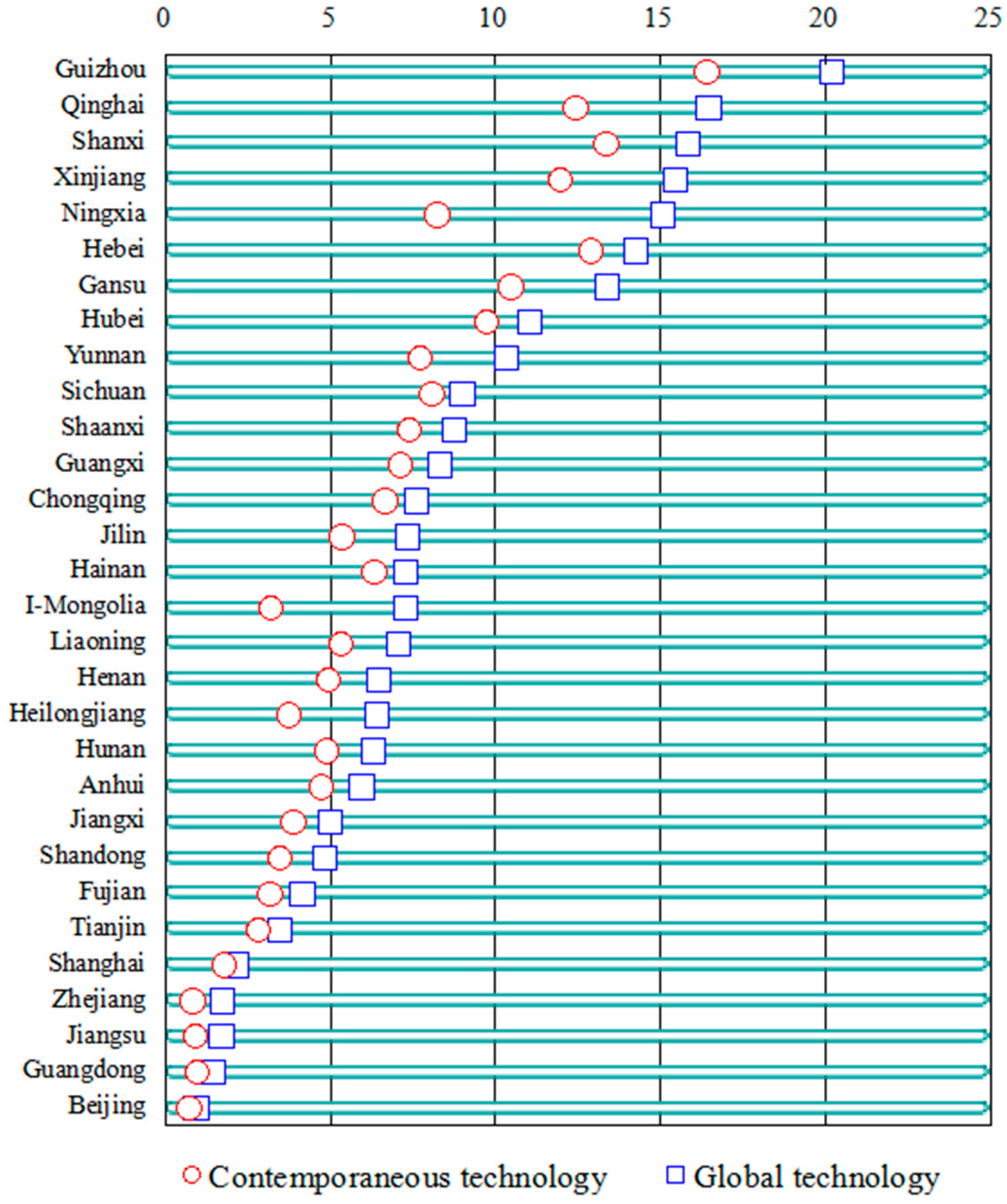
To conserve space, we only report the potential CO2 intensity reduction for China’s 30 provinces in 2012, shown in Figure 2. The potential CO2 intensity reduction is much higher in poorer western provinces, when compared to other provinces in China. Under the contemporaneous technology scenario, the potential CO2 intensity reduction in the western provinces, such as Guizhou, Qinghai, Shanxi, Xinjiang, and Ningxia, is 201.9, 164.5, 158.2, 154.6 and 150.8 thousand tons per billion RMB (2005 price), respectively, while the potential CO2 intensity reduction in the eastern provinces, such as Shanghai, Zhejiang, Jiangsu, Guangdong, and Beijing, is merely 21.3, 17.2, 17.0, 14.1 and 9.3 thousand tons per billion RMB (2005 price), respectively. This implies that there is a large potential for CO2 intensity reduction in China’s western provinces.
It can also be observed that the potential abasement of CO2 intensity under the global technology scenario is larger than that under the contemporaneous technology scenario. Moreover, the gap of potential reduction in CO2 intensity between the two different scenarios is larger in China’s poorer western provinces. In those western provinces such as Guizhou, Qinghai, Xingjiang, and Ningxia, the amount of potential CO2 intensity reduction under the global technology scenario is 164.1, 124.3, 119.6 and 82.2 thousand tons per billion RMB (2005 price), respectively; being 37.8, 40.3, 35.0, 68.6 and 41.0 thousand tons per billion RMB (2005 price) higher than those under the contemporaneous technology scenario. In contrast, in the eastern provinces such as Beijing, Guangdong, Jiangsu, Zhejiang, and Shanghai, the potential CO2 intensity reduction under the global technology scenario is 7.1, 9.4, 8.9, 8.2 and 17.7 thousand tons per billion RMB (2005 price), respectively; being merely 2.2, 4.7, 8.0, 9.1, 3.5 thousand tons per billion RMB (2005 price) higher than those under the contemporaneous technology scenario. That is because the eastern provinces are better off, and are more likely to absorb external technologies or invent advanced energy-saving technologies.

4. Conclusions

The Chinese government considers CO2 intensity to be one of the most important references for designing its energy and environmental policies. Understanding and analyzing the driving factors of CO2 intensity in China and its regions, are therefore of vital importance. An increasing number of research papers place an emphasis on analyzing the factors influencing China’s CO2 intensity. However, very few of them have paid attention to the variation in China’s regions. To the best of our knowledge, this paper is the first attempt to explore the change of CO2 intensity in China, as well as in its provinces. To serve this purpose, we propose a modification of the decomposition model of Kim and Kim [24], which integrates the strengths of IDA and PDA. Moreover, we also calculate the potential reduction of CO2 intensity for China as a whole and its provinces. Using a panel data set including China’s 30 provinces during the period of 2006–2012, empirical analysis is conducted and meaningful results are obtained accordingly.
With regards to China as a whole, DPEI (potential energy intensity change) was the dominant driving factor of the decrease in CO2 intensity, which contributed to a total reduction of 19.8% and 3.6% per year. DEMF (CO2 emission factor change), DEC (energy efficiency change), and DSTR (industrial structure change) were also contributing factors to the abatement of CO2 intensity. By contrast, DBPC (energy-saving technology change) and DEMX (energy mix change) did not lead to a decrease in CO2 intensity.
When it comes to the provincial level, some mixed pictures emerge. CO2 intensity in all of the provinces, excluding Xinjiang and Hainan, exhibited a decrease in CO2 intensity during the period of 2006–2012. For these provinces, the CO2 intensity reduction was mainly driven by DPEI (potential energy intensity change). DEC (energy efficiency change) and DEMF (CO2 emission factor change) also played positive roles in the CO2 intensity reduction for most provinces. The best performers in DPEI, DEC, and DEMF, were Hunan (0.637), Beijing (0.727), and Sichuan (0.785), respectively. Only four provinces, Shanghai (0.882), Guangdong (0.921), Beijing (0.96), and Tianjin (0.99), had positive contributions of energy-saving technology for the reduction of CO2 intensity, which suggests that the Chinese government should promote technology diffusion among the regions, helping those which are less developed to also introduce advanced technology.
In terms of the CO2 intensity reduction potential, China showed a narrowing possibility year by year. In 2012, the potential reduction under the global technology and the contemporaneous technology scenarios are calculated as 59.1 and 46.0 thousand tons per billion RMB (2005 price), decreasing from 83.7 and 69.3 thousand tons per billion RMB (2005 price), respectively. The provincial variations are also presented. Provinces in the western area generally showed a relatively large potential reduction for CO2 intensity, while those in the eastern area evidenced a small amount.
Finally, it should be pointed out that this paper focuses on exploring change in China’s carbon intensity using a decomposition method. We attribute the change of carbon intensity to several predefined effects. However, we have not answered the question of what drives the change of the decomposed components. This question requires great efforts in developing a unified model with economic foundations and collecting more related data. It should be further analyzed in future studies.

Acknowledgments

Kerui Du acknowledges financial support by National Natural Science Foundation of China (No. 71603148), Shandong Provincial Natural Science Foundation, China (No. ZR2016GB10), China Postdoctoral Science Foundation (No. 2016M590627), the Fundamental Research Funds of Shandong University. Boqiang Lin acknowledges financial support by Xiamen University—Newcastle University Joint Strategic Partnership Fund, the Grant for Collaborative Innovation Center for Energy Economics and Energy Policy (No. 1260-Z0210011), and Xiamen University Flourish Plan Special Funding (No. 1260-Y07200). We thank four anonymous reviewers for their helpful comments and suggestions which led to an improved version of this paper.

Author Contributions

Kerui Du, Boqiang Lin and Chunping Xie conceived, designed, prepared, and revised the paper together. All authors read and approved the final manuscript.

Conflicts of Interest

The authors declare no conflict of interest.

References

  1. Vaninsky, A. Factorial decomposition of CO2 emissions: A generalized Divisia index approach. Energy Econ. 2014, 45, 389–400. [Google Scholar] [CrossRef]
  2. Liu, L.-C.; Wang, J.-N.; Wu, G.; Wei, Y.-M. China’s regional carbon emissions change over 1997–2007. Int. J. Energy Environ. 2010, 1, 161–176. [Google Scholar]
  3. Wu, L.; Kaneko, S.; Matsuoka, S. Driving forces behind the stagnancy of China’s energy-related CO2 emissions from 1996 to 1999: The relative importance of structural change, intensity change and scale change. Energy Policy 2005, 33, 319–335. [Google Scholar] [CrossRef]
  4. Wu, L.; Kaneko, S.; Matsuoka, S. Dynamics of energy-related CO2 emissions in China during 1980 to 2002: The relative importance of energy supply-side and demand-side effects. Energy Policy 2006, 34, 3549–3572. [Google Scholar] [CrossRef]
  5. Xu, B.; Lin, B. How industrialization and urbanization process impacts on CO2 emissions in China: Evidence from nonparametric additive regression models. Energy Econ. 2015, 48, 188–202. [Google Scholar] [CrossRef]
  6. Zhang, M.; Mu, H.; Ning, Y. Accounting for energy-related CO2 emission in China, 1991–2006. Energy Policy 2009, 37, 767–773. [Google Scholar] [CrossRef]
  7. Fan, Y.; Liu, L.-C.; Wu, G.; Tsai, H.-T.; Wei, Y.-M. Changes in carbon intensity in China: Empirical findings from 1980–2003. Ecol. Econ. 2007, 62, 683–691. [Google Scholar] [CrossRef]
  8. Chen, S. The abatement of carbon dioxide intensity in China: Factors decomposition and policy implications. World Econ. 2011, 34, 1148–1167. [Google Scholar] [CrossRef]
  9. Su, B.; Ang, B.W. Multiplicative decomposition of aggregate carbon intensity change using input-output analysis. Appl. Energy 2015, 154, 13–20. [Google Scholar] [CrossRef]
  10. Tan, Z.; Li, L.; Wang, J.; Wang, J. Examining the driving forces for improving China’s CO2 emission intensity using the decomposing method. Appl. Energy 2011, 88, 4496–4504. [Google Scholar] [CrossRef]
  11. Zhao, X.; Burnett, J.W.; Fletcher, J.J. Spatial analysis of China province-level CO2 emission intensity. Renew. Sustain. Energy Rev. 2014, 33, 1–10. [Google Scholar] [CrossRef]
  12. Wang, K.; Zhang, X.; Wei, Y.-M.; Yu, S. Regional allocation of CO2 emissions allowance over provinces in China by 2020. Energy Policy 2013, 54, 214–229. [Google Scholar] [CrossRef]
  13. Zhang, W.; Li, K.; Zhou, D.; Zhang, W.; Gao, H. Decomposition of intensity of energy-related CO2 emission in Chinese provinces using the LMDI method. Energy Policy 2016, 92, 369–381. [Google Scholar] [CrossRef]
  14. Xu, S.; Han, H.; Zhang, W.; Zhang, Q.; Long, R.; Chen, H.; He, Z. Analysis of regional contributions to the national carbon intensity in China in different five-year plan periods. J. Clean. Prod. 2017, 145, 209–220. [Google Scholar] [CrossRef]
  15. Xu, X.Y.; Ang, B.W. Index decomposition analysis applied to CO2 emission studies. Ecol. Econ. 2013, 93, 313–329. [Google Scholar] [CrossRef]
  16. Ang, B.W. Decomposition analysis for policymaking in energy: Which is the preferred method? Energy Policy 2004, 32, 1131–1139. [Google Scholar] [CrossRef]
  17. Ang, B.W.; Liu, N. Energy decomposition analysis: IEA model versus other methods. Energy Policy 2007, 35, 1426–1432. [Google Scholar] [CrossRef]
  18. Wang, C. Decomposing energy productivity change: A distance function approach. Energy 2007, 32, 1326–1333. [Google Scholar] [CrossRef]
  19. Li, M. Decomposing the change of CO2 emissions in China: A distance function approach. Ecol. Econ. 2010, 70, 77–85. [Google Scholar] [CrossRef]
  20. Wang, Q.; Chiu, Y.-H.; Chiu, C.-R. Driving factors behind carbon dioxide emissions in China: A modified production-theoretical decomposition analysis. Energy Econ. 2015, 51, 252–260. [Google Scholar] [CrossRef]
  21. Zhang, X.-P.; Tan, Y.-K.; Tan, Q.-L.; Yuan, J.-H. Decomposition of aggregate CO2 emissions within a joint production framework. Energy Econ. 2012, 34, 1088–1097. [Google Scholar] [CrossRef]
  22. Zhou, P.; Ang, B.W. Decomposition of aggregate CO2 emissions: A production-theoretical approach. Energy Econ. 2008, 30, 1054–1067. [Google Scholar] [CrossRef]
  23. Lin, B.; Du, K. Decomposing energy intensity change: A combination of index decomposition analysis and production-theoretical decomposition analysis. Appl. Energy 2014, 129, 158–165. [Google Scholar] [CrossRef]
  24. Kim, K.; Kim, Y. International comparison of industrial CO2 emission trends and the energy efficiency paradox utilizing production-based decomposition. Energy Econ. 2012, 34, 1724–1741. [Google Scholar] [CrossRef]
  25. Oh, D.-H. A global Malmquist-Luenberger productivity index. J. Prod. Anal. 2010, 34, 183–197. [Google Scholar] [CrossRef]
  26. Pastor, J.T.; Lovell, C.A.K. A global Malmquist productivity index. Econ. Lett. 2005, 88, 266–271. [Google Scholar] [CrossRef]
  27. Wang, H.; Zhou, P.; Zhou, D.Q. Scenario-based energy efficiency and productivity in China: A non-radial directional distance function analysis. Energy Econ. 2013, 40, 795–803. [Google Scholar] [CrossRef]
  28. Wu, F.; Fan, L.W.; Zhou, P.; Zhou, D.Q. Industrial energy efficiency with CO2 emissions in China: A nonparametric analysis. Energy Policy 2012, 49, 164–172. [Google Scholar] [CrossRef]
  29. China, Premium Database. Available online: http://www.ceicdata.com. (accessed on 7 Aprial 2015).
  30. National Bureau of Statistics of China. China Energy Statistical Yearbook 2007; China Statistics Press: Beijing, China, 2007. (In Chinese)
  31. National Bureau of Statistics of China. China Energy Statistical Yearbook 2008; China Statistics Press: Beijing, China, 2008. (In Chinese)
  32. National Bureau of Statistics of China. China Energy Statistical Yearbook 2009; China Statistics Press: Beijing, China, 2009. (In Chinese)
  33. National Bureau of Statistics of China. China Energy Statistical Yearbook 2010; China Statistics Press: Beijing, China, 2010. (In Chinese)
  34. National Bureau of Statistics of China. China Energy Statistical Yearbook 2011; China Statistics Press: Beijing, China, 2011. (In Chinese)
  35. National Bureau of Statistics of China. China Energy Statistical Yearbook 2012; China Statistics Press: Beijing, China, 2012. (In Chinese)
  36. National Bureau of Statistics of China. China Energy Statistical Yearbook 2013; China Statistics Press: Beijing, China, 2013. (In Chinese)
  37. Liu, Z.; Geng, Y.; Lindner, S.; Guan, D. Uncovering China’s greenhouse gas emission from regional and sectoral perspectives. Energy 2012, 45, 1059–1068. [Google Scholar] [CrossRef]
  38. National Bureau of Statistics of China. China Statistical Yearbook 2014; China Statistics Press: Beijing, China, 2014. (In Chinese)
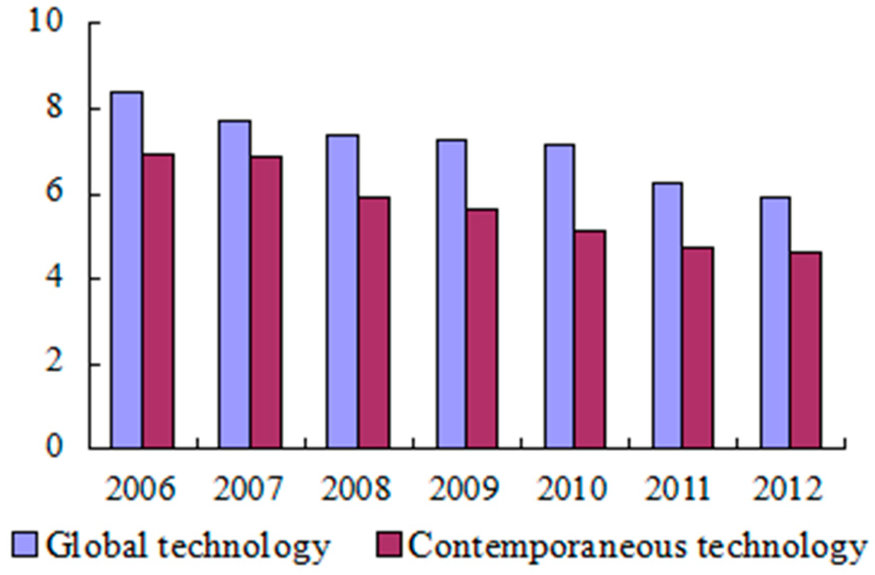
Figure 1. The potential CO2 intensity reduction for China: 2006–2012. Unit: 10 thousand tons/billion RMB (2005 price).
Sustainability 09 00296 g001
Figure 2. The potential CO2 intensity reduction for China’s 30 provinces in 2012. Unit: 10 thousand tons/billion RMB (2005 price).
Sustainability 09 00296 g002
Table 1. The definitions of the decomposed components.
SymbolDescription
DEMFthe CO2 emission factor effect
DEMXthe effect of energy mix change
DPEIthe effect of potential energy intensity change
DSTRindustrial structure effect, accounting for the impact from output composition change
DBPCthe impact from technological change in energy use
DECthe effect of energy efficiency change
DROSthe effect of regional output structure change
Table 2. The change of CO2 intensity and effects of contributing factors in China.
YearDtotDEMFDEMXDSTRDROSDPEIDECDBPC
2006–20070.9500.9841.0151.0051.0000.9561.0170.974
2007–20080.9580.9990.9991.0061.0010.9570.9641.032
2008–20090.9350.9800.9930.9791.0010.9630.9991.019
2009–20100.9600.9910.9911.0141.0010.9540.9841.026
2010–20110.9971.0071.0431.0021.0040.9950.9780.970
2011–20120.9360.9860.9970.9881.0030.9581.0090.993
Geometric mean0.9560.9911.0060.9991.0020.9640.9921.002
2006–20120.7620.9461.0380.9951.0100.8020.9521.013
Table 3. The change of CO2 intensity and effects of contributing factors in China’s 30 provinces between 2006 and 2012.
ProvinceDtotDEMFDEMXDSTRDPEIDECDBPC
Anhui0.7120.9650.9901.1460.6630.9651.017
Beijing0.5450.8171.1080.9310.9260.7270.960
Chongqing0.7690.9210.9671.0160.7991.0281.033
Fujian0.7480.9781.0391.0020.7980.9031.021
Gansu0.8611.0220.9500.9640.9060.9881.027
Guangdong0.7400.9431.0430.9780.8650.9660.921
Guangxi0.7760.9121.0751.1290.7170.9551.024
Guizhou0.6220.9111.0090.9590.6601.0191.050
Hainan1.1551.1030.9650.8881.2370.9861.002
Hebei0.7830.9470.9630.9840.8161.0621.006
Heilongjiang0.7780.9730.9900.9330.8650.9611.042
Henan0.6800.9311.0561.0280.7020.9351.026
Hubei0.7440.9010.8881.0530.7431.1551.029
Hunan0.6460.9381.0941.0810.6370.8751.045
I-Mongolia0.8931.0541.1261.0910.8290.8011.039
Jiangsu0.7960.9661.0770.9120.9030.9131.016
Jiangxi0.7570.9051.1371.0810.7540.8891.014
Jilin0.6570.9761.0801.0920.6410.8871.003
Liaoning0.7800.9801.2351.0340.7870.7851.008
Ningxia0.9010.9931.0600.9560.9500.9061.041
Qinghai0.9440.9100.9831.1010.8621.0731.036
Shaanxi0.7680.9190.9650.9930.8071.0371.042
Shandong0.7580.9491.0480.9260.8480.9401.033
Shanghai0.6850.9600.9980.8610.8951.0510.882
Shanxi0.7770.9851.1320.9810.8030.8581.031
Sichuan0.6880.7850.8801.0990.6781.3231.012
Tianjin0.6330.9900.8590.9620.7561.0350.990
Xinjiang1.2161.0121.1950.9541.2500.8091.042
Yunnan0.8200.9731.0340.9280.8960.9491.032
Zhejiang0.7240.9130.9950.9520.8180.9941.030