Effective Height of a Floor Splitter Anti-Vortex Device under Varying Flow Conditions

Abstract

A pump station is a crucial flood control facility for mitigating inundation of urban lowland areas. Securing a site to increase the capacity of a pump station or to maximize the discharge capacity of the pump sump in an urban area is difficult because of various limitations. Moreover, adding a facility to improve the pump capacity of a pump station may affect flow characteristics, e.g., unexpected increases in flow velocity and vorticity, and cause severe problems in pump station operation. To solve those problems, anti-vortex devices (AVDs) have been developed and adopted according to the appropriate design standards. The Korean design criteria for AVDs are based on experience and the standards of other countries because of the lack of adequate data on AVDs. In this study, flow in the sump was numerically simulated at various AVD heights to obtain data for improving the design and efficiency of a pump station. Consequently, the appropriate height for the AVD and changes in the flow pattern and vortex in the pump sump were determined and compared with 12 cases of inflow conditions with respect to the vertical location.

1. Introduction

Urban floods due to severe rainstorms have become a serious problem in many countries. Furthermore, lowlands at urban riverfronts are very vulnerable to floods; most flood damage typically occurs in these areas. Thus, reliable and effective urban flood control facilities are needed to improve flood safety in lowlands. Various flood control facilities can be adopted as structural countermeasures to mitigate flood risk in urban lowlands. A pump station is a crucial and efficient flood control facility that discharges the water inundating the lowland into the watershed.

Abnormally heavy rainfall because of climate change is increasing the occurrence of floods, which threaten people’s lives and properties in flood-vulnerable areas. To minimize flood damage, a pump station must be able to manage incoming flow over its design capacity. A wide range of flood conditions can occur during pumping operations depending on variations in the river water level and changes in the sewage flow. This variation renders the sump pump unsteady and unstable, which decreases pump capacity through cavitation, flow separation, pressure loss, and variation. In particular, air-entrained free-surface and subsurface vortices in pump sumps severely damage the pump system. Various numerical and experimental studies have focused on preventing the degradation of pump station capacity because of abnormal conditions in the sump pump.

For instance, Arboleda and El-Fadel [1] performed a case study on sump design by using a hydraulic model and investigated the effect of several design features and site constraints on hydraulic performance and sump configuration. Bauer and Nakato [2] experimentally studied the flow field formed in a pump sump; they varied the operating conditions and determined the consequent effect on the formation of vortices around a bell mouth. Constantinu and Patel [3] applied a numerical k − ε turbulence model to determine the location, size, and strength of vortices. They demonstrated that the numerical model can reproduce the flow pattern in a sump pump but stated that the results should be validated through experimental observations.

Rajendran et al. [4] installed a vertical suction pipe in a rectangular channel, measured the flow characteristics through a particle image velocimetry (PIV) experiment, and performed a numerical analysis. Similarly, through PIV, Rajendran and Patel [5] performed detailed measurements of vortices in the pump intake bay of a laboratory model comprising a vertical intake pipe with a bell mouth in order to improve the understanding of vortex formation in the bay. Their experiments demonstrated the utility of PIV in obtaining quantitative information on the number, location, and size of vortices, which is required to develop and validate numerical models of pump intake flows. Nagahara et al. [6] comprehensively investigated the velocity distribution around submerged vortex cavitation in a pump intake through PIV. Choi [7] installed an experimental model of a suction cistern and used PIV to observe the flow characteristics in the sump.

Nagahara et al. [6] experimentally and numerically analyzed the flow structure around a suction pipe due to asymmetric flow velocity toward the water course direction in the suction cistern. The Turbomachinery Society of Japan (TSJ) [8] amended the standard for pump suction cisterns and reviewed the applicability of various numerical models for the same analysis target. Johansson et al. [9] conducted a model study on a sump through a physical test and by applying computational fluid dynamics (CFD) and demonstrated how hydraulic models can be used to identify unacceptable flow conditions, such as surface vortices, high swirls, pre-rotation, and non-uniform axial velocity distribution at the bell mouth. They used the results to derive modifications for improving the hydraulic performance in the pump intakes of both circulating water and cooling water. Okamura et al. [10] conducted a hydraulic experiment similar to the benchmark test of TSJ and verified the accuracy of various numerical models. Park and Roh [11] reproduced the flow of the Japanese standard simple sump model of TSJ by using a CFD model and observed the generation of free surface and underwater vortices. Kim et al. [12] used the ANSYS CFX (ANSYS, Inc., Canonsburg, PA, USA) model to analyze the effects of the gap between an underwater cargo pump inlet and pump sump on suction performance. Choi et al. [13] simulated the flow homogeneity of pump stations with multiple pump sumps through numerical analysis and analyzed the effects of an anti-vortex device (AVD) on the flow field. Choi et al. [14] reproduced the benchmark experiment of the TSJ by using a numerical model and analyzed the effects of an AVD on pump efficiency by considering additional AVDs.

Various numerical and experimental techniques have been developed to reproduce the flow characteristics of a pump station sump in order to prevent vortices. However, the design of pump stations under a design constraint needs further development; this is essential because pump stations have varying flow conditions. Previous studies have usually focused on steady flow conditions for the incoming and outgoing flows of the pump station. Thus, the currently available design techniques, such as the Turbomachinery Society of Japan [8] and Hydraulic Institute [15] for sump pumps are inappropriate for operation under varying flood conditions and must be tested under unsteady flow conditions. In this study, a numerical model was applied to analyze the changes in flow characteristics under varying flow conditions in order to determine the optimal height of the attached sump pump facility that effectively mitigates abnormal flow.

2. Numerical Model

2.1. Mathematical Formulation

ANSYS CFX was used in this study to reproduce the flow in the pump sump. CFX is a three-dimensional flow analysis program developed by ANSYS in which the user can make both structural and non-structural tetrahedral grids for efficient grid formation. ANSYS CFX is an element-based finite-volume method with second-order discretization schemes in space and time. ANSYS CFX uses a coupled solver, which solves the hydrodynamic equations (for u, v, w, and p) as a single system. It facilitates accurate flow analysis for the contact surface between a solid and liquid, such as the shear stress on the wall or bottom of a channel. The analysis is governed by the following continuity and momentum equations:

$$\frac{\partial \rho }{\partial t}+\nabla ·\left(\rho U\right)=0$$

(1)

$$\frac{\partial \left(\rho U\right)}{\partial t}+\nabla ·\left(\rho U\times U\right)=-\nabla p+\nabla ·\tau +S_M$$

(2)

$$\tau = \mu \left[\nabla U+{\left(\nabla U\right)}^T-\frac{2}{3}\delta \nabla ·U\right]$$

(3)

Here, ρ is the density of water (kg/m³), U is the flow vector, p is the pressure, τ is a stress tensor related to the strain rate, and S_M is an external momentum-generation term.

The shear stress transport (SST) model was applied to the turbulence model for calculating the steady state conditions. The SST model is an improved turbulence closure model that combines the advantages of the k – ε and k – ω models to achieve a wide range of applicability. To this end, the SST model adopts the blending function F1, which equals 1 near the solid surface and 0 for the flow domain where wall friction is not dominant. It solves the k − ω equations in the near-wall region and the k – ε equations for the rest of the flow. Through this approach, the favorable near-wall performance of the k – ω model can be used without potential errors resulting from its free stream sensitivity. In addition, the SST model features a modification to the definition of eddy viscosity, which can be interpreted as a variable c_μ; by contrast, c_μ in the k – ε model is constant [16]. This modification is required to accurately simulate the onset of separation under pressure gradients. In a recent NASA technical memorandum, the SST model was rated as the most accurate model in its class [17]. The SST model is similar to the standard k − ω model; its equations are as follows:

$$\frac{\partial }{\partial t}\left(\rho k\right)+\frac{\partial }{\partial x_i}\left(\rho k{u}_i\right)=\frac{\partial }{\partial x_j}\left({\mathsf{\Gamma }}_k\frac{\partial k}{\partial x_j}\right)+G_k-Y_k$$

(4)

$$\frac{\partial }{\partial t}\left(\rho \omega \right)+\frac{\partial }{\partial x_i}\left(\rho \omega u_i\right)=\frac{\partial }{\partial x_j}\left({\mathsf{\Gamma }}_{\omega }\frac{\partial \omega }{\partial x_j}\right)+G_{\omega }-Y_{\omega }+D_{\omega }$$

(5)

Here, ρ is the density, k is the turbulent kinetic energy, and ω is the specific dissipation rate. G_k represents the generation of turbulent kinetic energy due to mean velocity gradients. G_ω represents the generation of ω. Γ_k and Γ_ω represent the effective diffusivities of k and ω, respectively. Y_k and Y_ω are the dissipations of k and ω due to turbulence. D_ω represents the cross-diffusion term.

2.2. Model Validation

The adopted model was applied to a benchmark test case for validation. Okamura et al. [10] experimentally investigated the generation of a stationary surface vortex, non-stationary surface vortex, and stationary subsurface vortex. The width of the channel was 300 mm, the suction pipe diameter was 145 mm, and the inlet was installed 100 mm from the bottom of the channel and 110 mm from the back wall. The center of the suction pipe was shifted 10 mm from the central line of the channel to produce a nonhomogeneous flow. The water level was 230 mm, and the output was 1.0 m³/min (Figure 1).

The flow domain is discretized into tetrahedron meshes of size 0.002–0.01 m. In this study, the first-order upwind scheme and the central differencing scheme were applied for stabilizing the convective term and the diffusion term, respectively. The RMS error of 10⁻⁵ was set as the criteria to obtain converged numerical solutions. Due to the large computational loads of a three-dimensional problem, the computation was distributed to 32 processors.

Figure 2 presents the numerical results of this study and the experimental observations of Okamura et al. [10] obtained using LS-PIV (large-scale Particle Image Velocimetry) along the observation line crossing the center of the inlet on the x-y plane at z = 85 mm from the channel bottom. The x-directional flow velocity results showed a better agreement with the observed flow velocity than did those of Okamura et al. [10], and the results for the y- and z-directional flow velocities showed marked improvement over those of Okamura et al. The vorticity was considerably larger than the results of the previous numerical simulations and observed values on the right side of the channel, but it was mostly similar to the previous numerical simulations and observed values at the center or on the left. Thus, we conclude that the numerical model implemented in this study can reasonably reproduce the flow characteristics on the suction side.

3. Numerical Investigation

3.1. Anti-Vortex Device in the Sump Pump

The splitter and fillets attached to the floor under the bell mouth are the typical AVD for reducing the vortices and pre-swirls in the pump sump. Figure 3 shows the AVD adopted in this study. This AVD has a bottom splitter to improve the flow characteristics near the bell mouth and side wall corner fillets to reduce the side wall vortices and swirls. The slope of each splitter and fillet is 45°, and its length from the back wall is 110 m. The effective height of the AVD was determined on the basis of the results of the numerical tests.

To determine the effective height of the splitter/fillet AVD, the additional flow conditions described in

Table 1. Numerical test cases and their flow depths and AVD heights.

Test Case	AVD Height (h/D)	Test Case	AVD Height (h/D)	Flow Depth (m)	Flow Depth (m)
Case 1-1	0.1	Case 1-1	Case 3-1	0.3	Case 3-1
Case 1-2		Case 1-2	Case 3-2	0.20	Case 3-2
Case 1-3		Case 1-3	Case 3-3	0.25	Case 3-3
Case 1-4		Case 1-4	Case 3-4	0.30	Case 3-4
Case 2-1	0.2	Case 2-1	Case 4-1	0.4	Case 4-1
Case 2-2		Case 2-2	Case 4-2	0.20	Case 4-2
Case 2-3		Case 2-3	Case 4-3	0.25	Case 4-3
Case 2-4		Case 2-4	Case 4-4	0.30	Case 4-4

were considered. The adopted AVD heights were set according to the ratio to the bell mouth diameter in the range 0.1–0.4. The flow depth range was 0.15–0.30 m with 0.05 m increments. Figure 4 describes the numerical domain and mesh for the numerical simulation that was created using the ANSYS meshing tool with mesh size criteria (edge size) of 2–5 mm.

3.2. Numerical Results

To analyze the effectiveness of AVD in the pump sump, the change in the flow characteristics of the quantitative and qualitative methods were compared. The vortex core was visualized and compared to illustrate the danger area (i.e., the area with high strength vorticity). A vortex can be defined as either a region or a line. Generally, line-based algorithms provide more compact representations of vortices and can easily distinguish between individual vortices in close proximity [18]. In this study, the helicity method reported by Levy et al. [19] was adopted to analyze the vorticity in the pump sump. 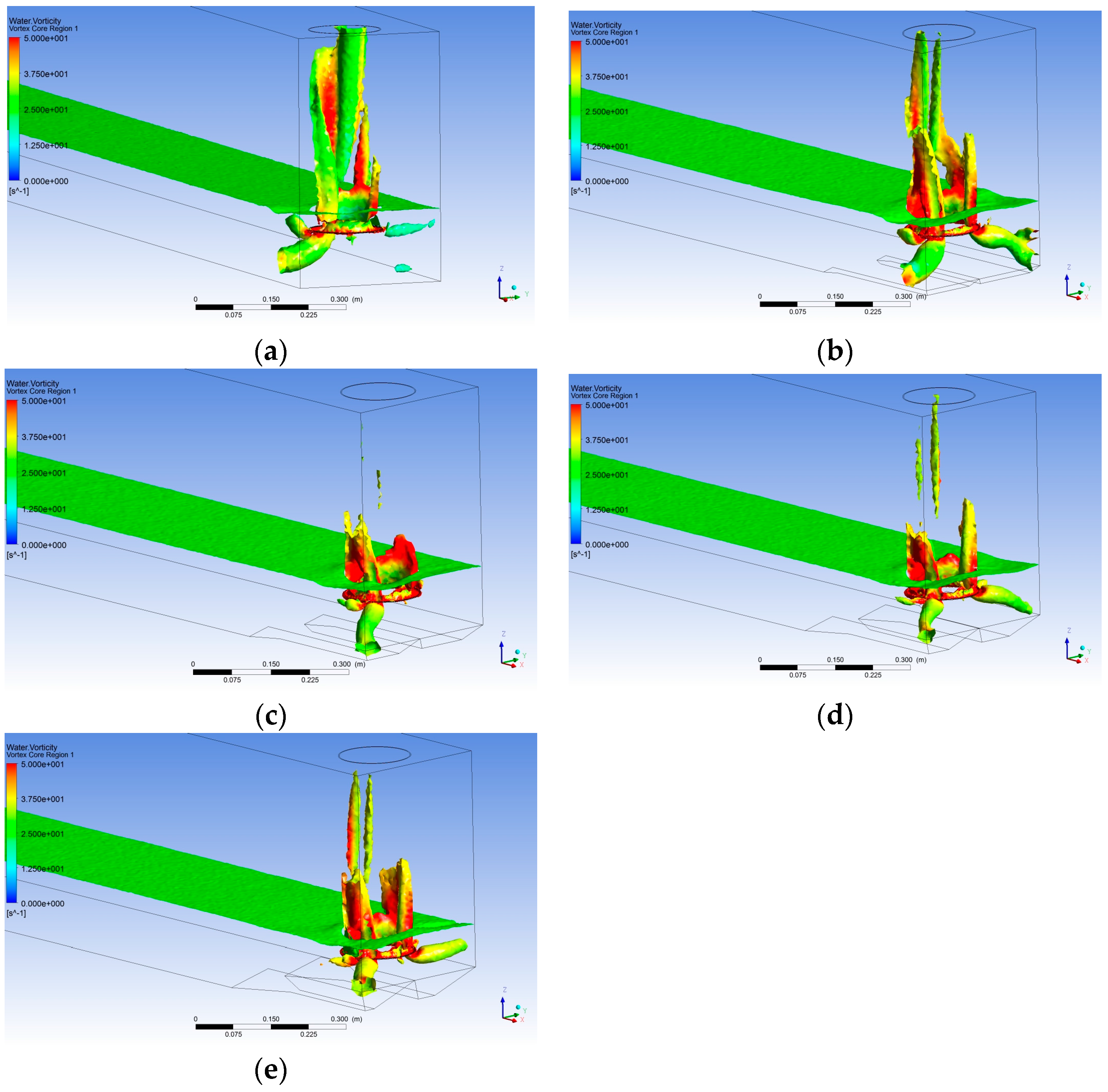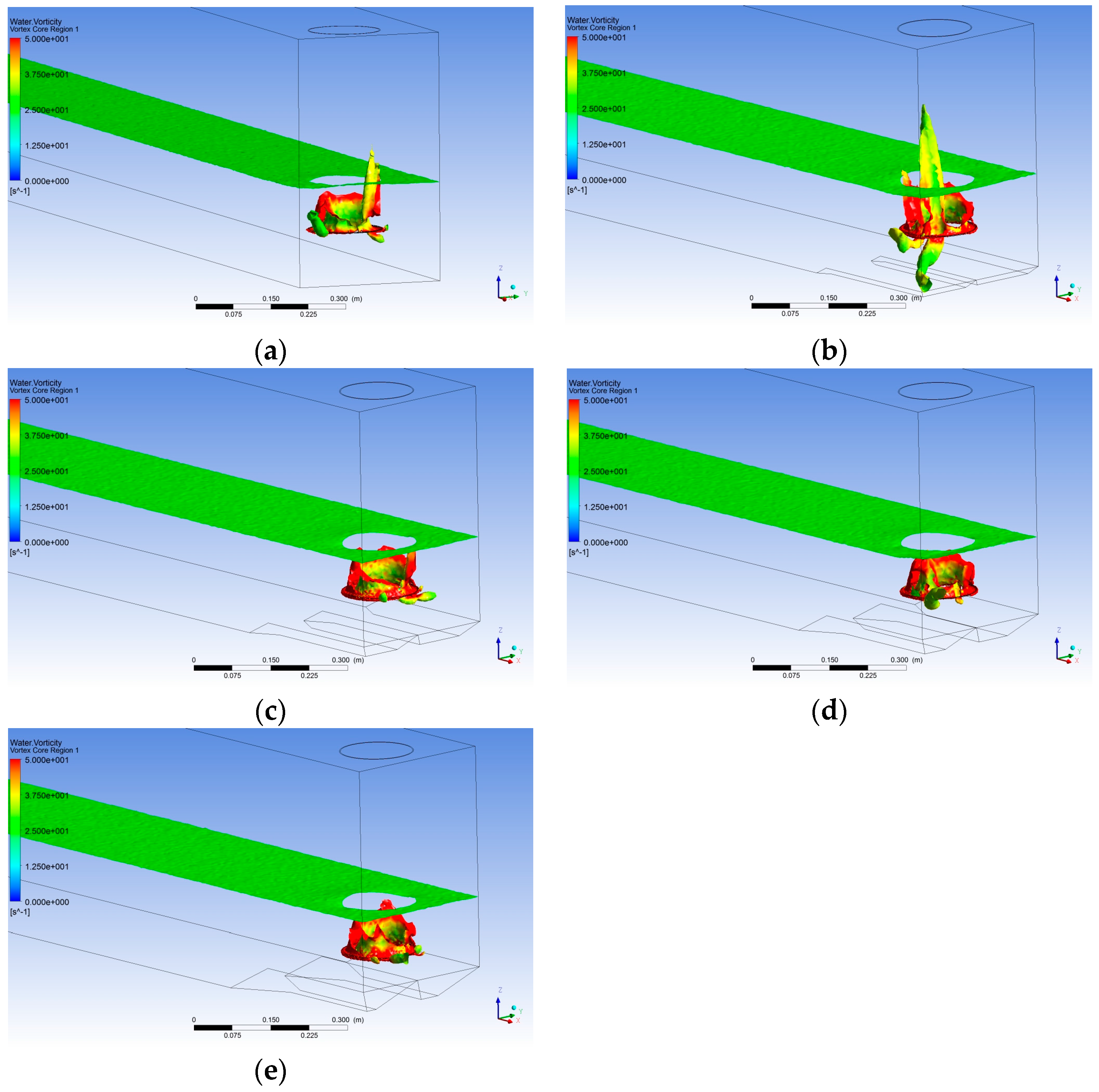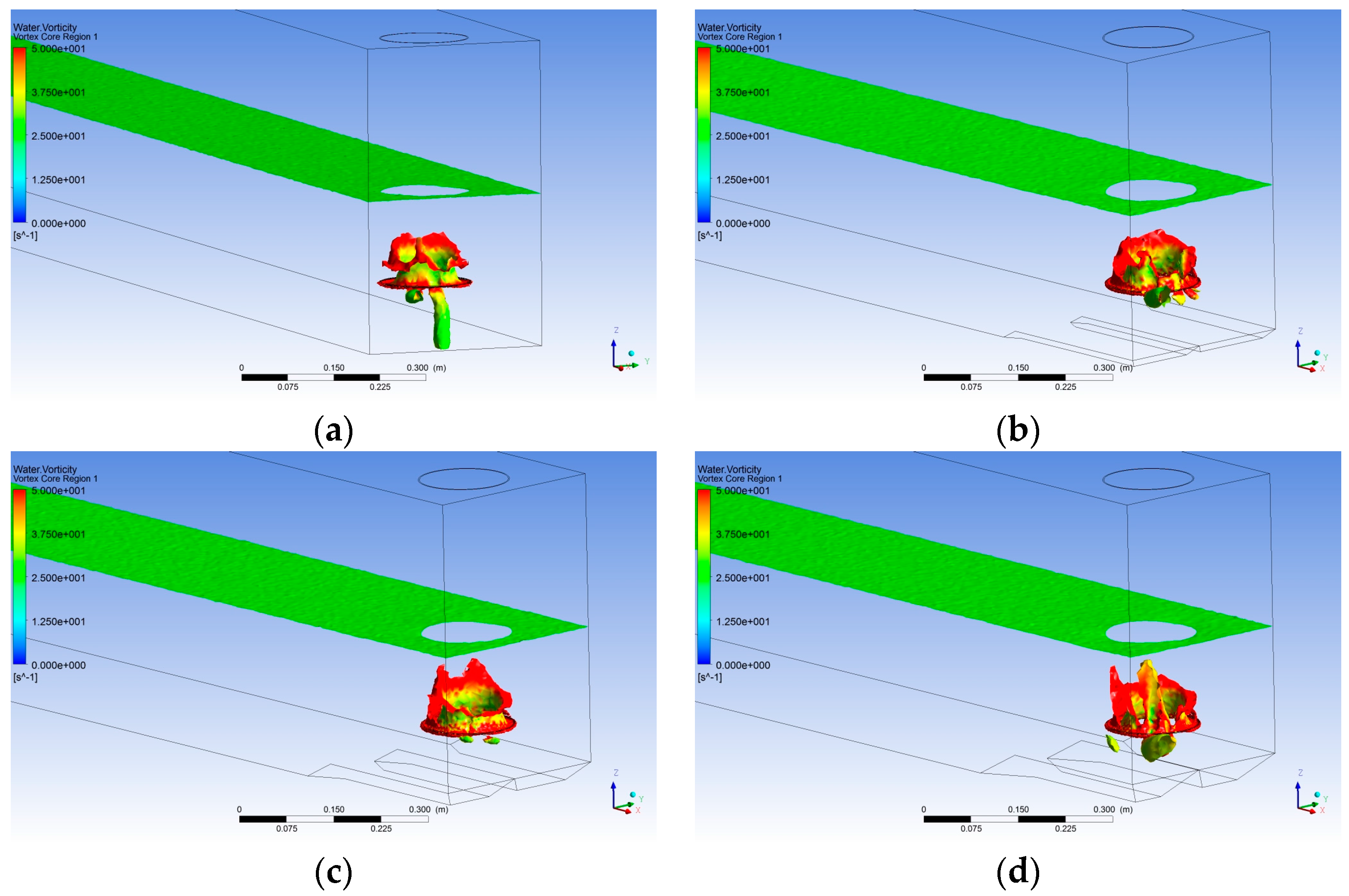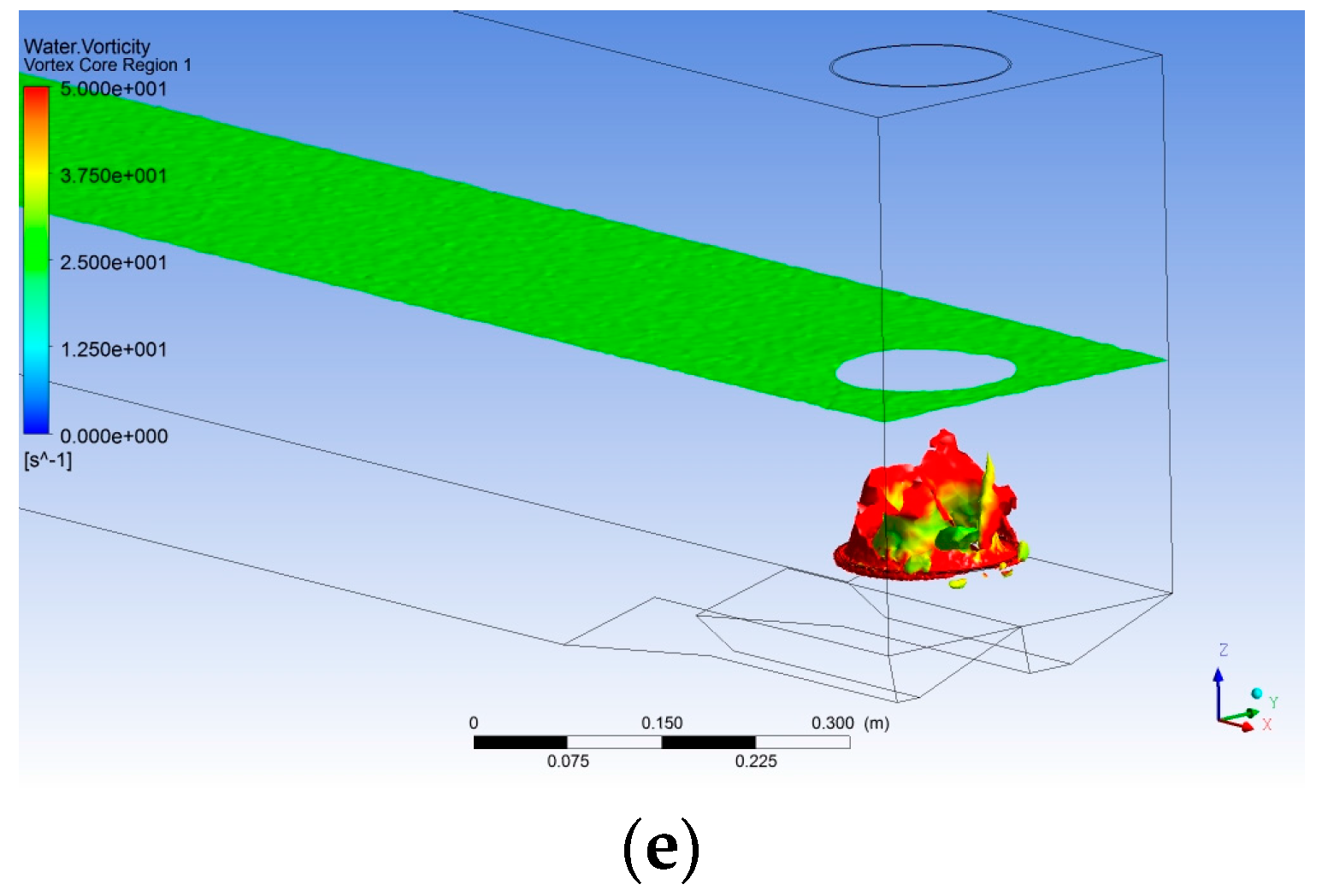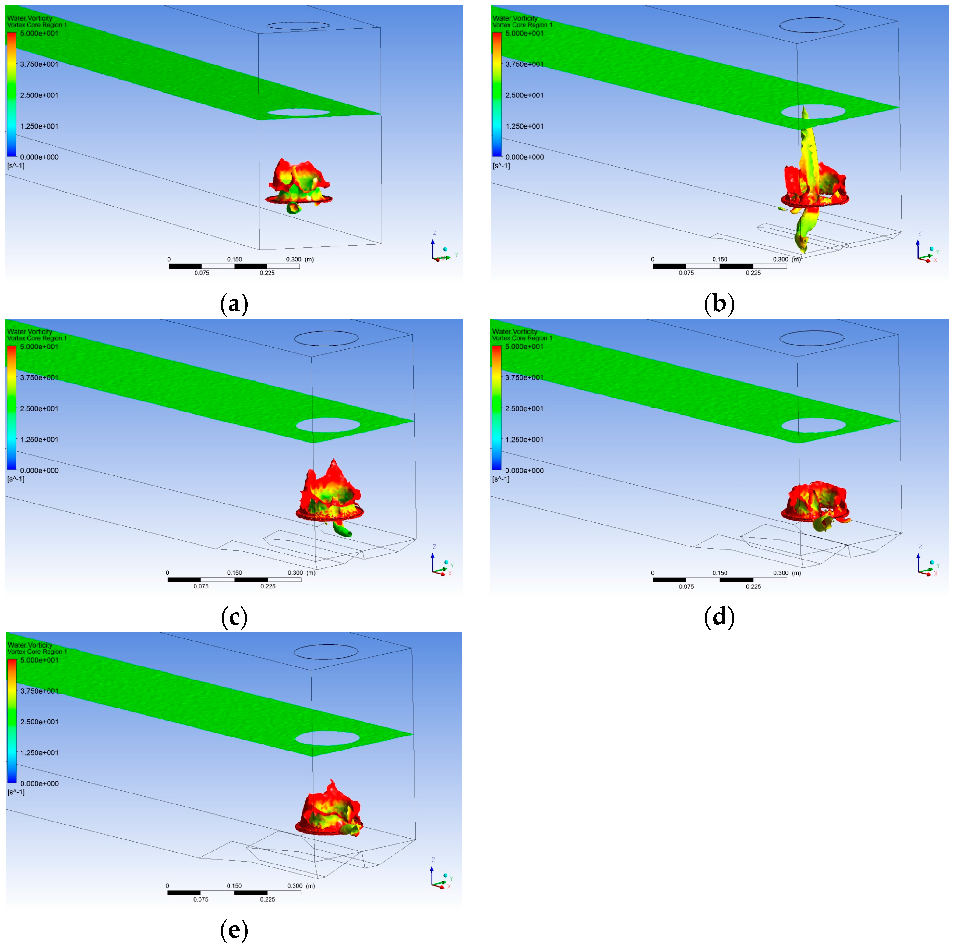Figure 5 shows the analyzed vortex zones under different AVD height conditions in a pump sump with an inflow depth of 0.15 m. The vortex core developed the near channel wall and affected flow in the outlet pipe. However, with variation in AVD height, the formed vortex region changed. The vortex region was minimized for AVD height d = 0.2D under the 0.15-m inflow depth condition. With further increase in AVD height, the vortex region becomes larger (Figure 6, Figure 7 and Figure 8).

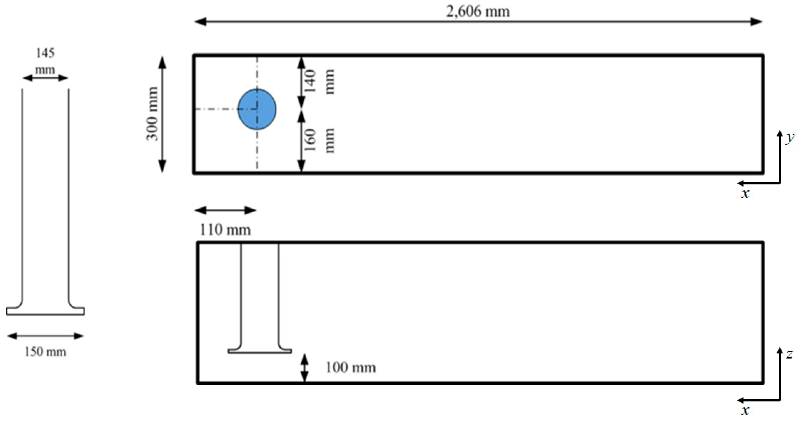
The changes in the flow velocity and vorticity were quantitatively compared along the four lines listed in

Table 2. Locations of lines for result comparisons.

Items	Line 1	Line 2	Line 3	Line 4
Surface height z from the bottom of the channel (mm)	25	50	75	100
Line direction	y-axis crossing the center of the inlet

. The chosen four lines are located under the bell mouth center along the y-axis, and the heights of lines are 25, 50, 75, and 100 mm from channel bottom. The comparison lines location were determined to analyze flow characteristic changes along the depth beneath the bell mouth center where is the most effective area for pump capacity.

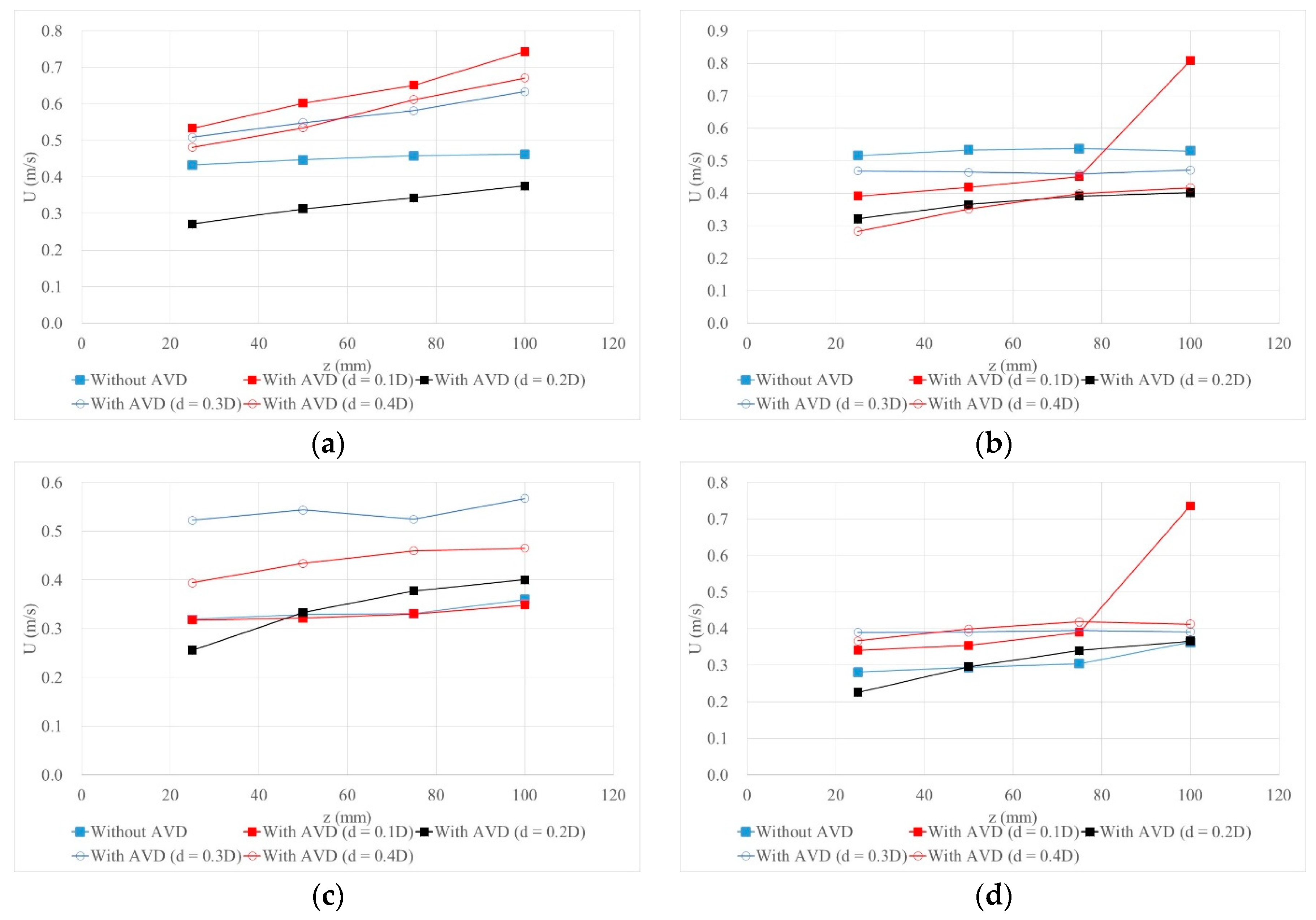
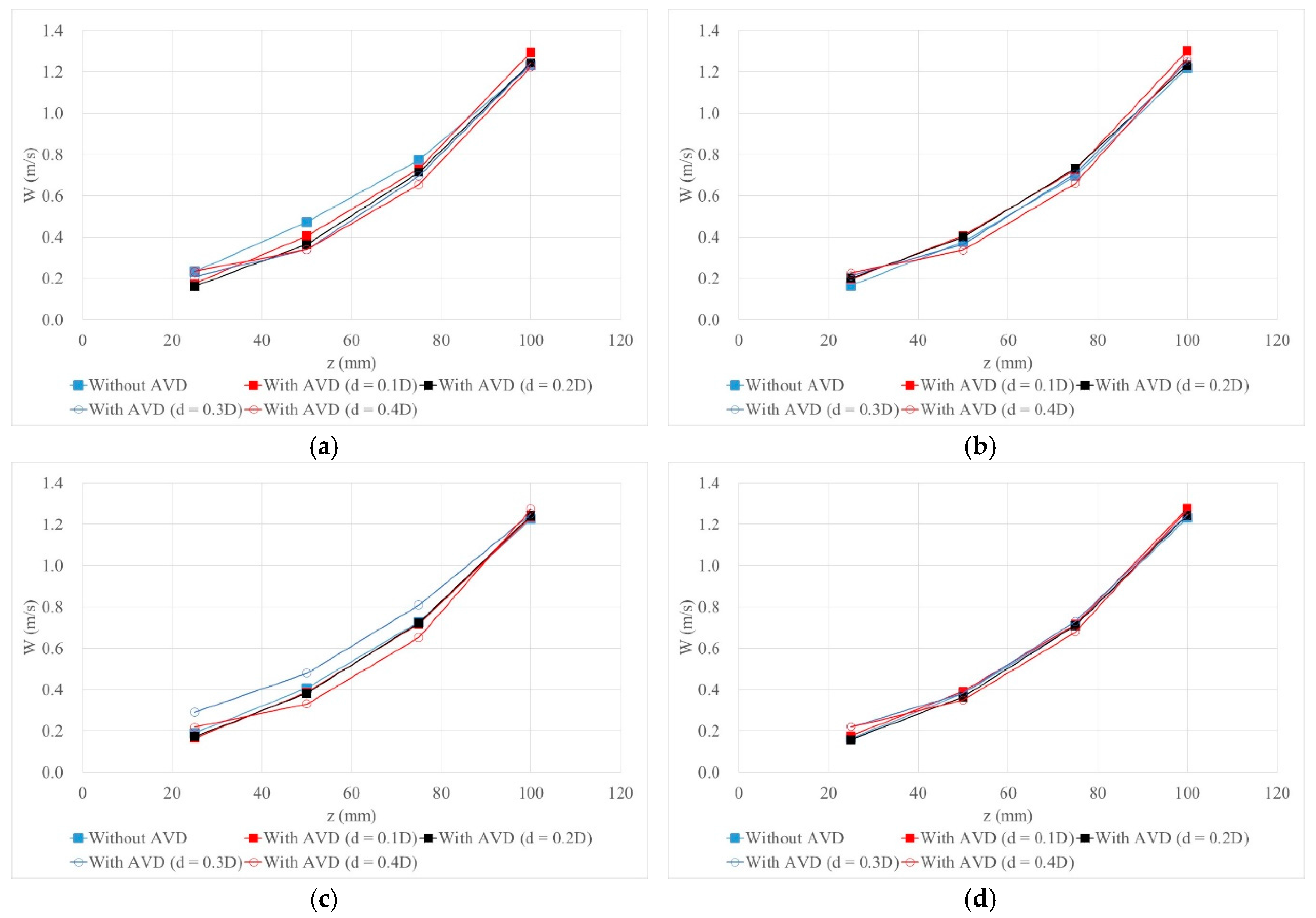
Figure 9 shows the numerical results of x-directional velocities along the four comparison lines under the numerical cases listed in Table 1. Figure 9a shows the numerical simulation results with the lowest inflow depth of H = 0.15 m. In all of the cases with AVD installations, the calculated velocities were compared with those in the no AVD case. It seemed that the decreased flow area due to AVD installation increased the approach velocity in the front of the bell mouth. However, when AVD height was 0.2D, the flow velocity decreased as depicted in Figure 9a. Figure 9b shows the numerical simulation results at the inflow depth of H = 0.20 m. In general, the flow velocity was reduced by the installed AVD. However, when the AVD height was 0.1D, the flow velocity near the bell mouth abruptly increased. It can be surmised that the inappropriate AVD height affects the approach flow streamline and causes a severe direction change. Figure 9c depicts the calculated x-directional velocity results under the numerical cases with an inflow depth of H = 0.25 m. When the AVD was present, it derived the increased flow velocity results. It showed the decrease in the flow velocity results only at the lowest comparison line with AVD of height 0.2D. It can be surmised that the bottom splitter changed the flow directions and the velocity in x-direction near channel bottom decreased and that of the upper area around the bell mouth increased. Figure 9d shows the numerical results with the deepest inflow depth of H = 0.30 m. When the AVD was installed in the sump, the flow velocity along the x-axis increased in general. However, when the installation height was 0.2D, the flow velocity near the channel bottom was decreased. Furthermore, when the AVD height was 0.1D, the flow velocity near the bell mouth abruptly increased. It can be surmised that the appropriate AVD height may decrease approach flow velocity similar to the AVD height d = 0.2D case, but if the AVD height is not appropriate the flow velocity may increase considerably around the bell mouth, as shown in the case of AVD height d = 0.1D.

Figure 10 shows the numerical results of the maximum y-directional velocities on the four comparison lines. Figure 10a shows the numerical results with the lowest inflow depth of H = 0.15 m. The calculated velocities generated similar value with the case without AVD installation, except the AVD height is d = 0.1D between the z is from 50 mm to 75 mm. In this region, the result for the case with AVD height d = 0.2D show slightly decreased velocity in the y-direction. In all cases, AVD installation derived velocity increase. It seems that the decreased flow area due to AVD installation may worsen flow characteristics near the bell mouth. It shows the increased flow velocity consistently with the AVD height d = 0.1D. Thus, it can be surmised that the AVD height is insufficient to control flow characteristics in the pump sump, and AVD may cause unintended flow condition changes. Figure 10b shows the numerically calculated y-directional flow velocities for the AVD installation case with inflow depth of H = 0.20 m. Very similar velocity distributions were obtained in most cases, and the calculated flow velocity is found to be slightly lower for AVD height d = 0.2D between z = 25 mm and 0.75 mm. However, the flow velocity was higher when the AVD height was 0.1D, similar to the results of inflow depth H = 0.15 m case. Increased velocity results are observed at z = 100 mm lines where the bell mouth is located. Figure 10c depicts the calculated y-directional velocity results under the numerical cases with inflow depth of H = 0.25 m conditions.

As shown in Figure 10c, the installation of AVD did not make a significant difference in velocity calculations, except in the case of AVD height of d = 0.3D in the region of z-direction from 25 mm to 75 mm. However, it showed increased velocity calculation results near the bell mouth in all AVD installation cases. Figure 10d shows a comparison of the numerical results of y-directional velocity with the deepest inflow depth of H = 0.30 m. It was observed that the AVD installation causes a slight velocity increase from z = 25 mm to 75 mm, except in the case of AVD height d = 0.2D. The maximum velocity increase was observed in the case of AVD height d = 0.1D. In all AVD installation cases, a velocity increase was observed on the bell mouth height. In the numerical results comparisons of the y-directional velocity change, the velocity was observed to increase owing to AVD installation around the bell mouth height. It is surmised that the velocity decrease by AVD installation cannot be expected in all areas in the pump sump, and unexpected flow velocity increase may occur near the bell mouth.

Figure 11 shows a comparison of z-directional velocity changes by AVD installation. Figure 11a shows the numerical simulation results with the lowest inflow depth of H = 0.15 m. In the overall cases with AVD installations, only a slight decrease in velocity was observed. The velocity decrease was distinctly observed between z = 50 mm and 75 mm areas. Very similar velocity calculation results were observed near the bell mouth height, but little velocity increase is expected with an installation of AVD height d = 0.1D. Figure 11b depicts the numerical results of the z-directional velocity with an inflow depth of H = 0.20 m. In all of the cases, no significant velocity change was observed. This means that AVD installation cannot affect the z-directional velocity in all cases. Figure 11c shows the comparison of maximum z-directional velocity on the comparison lines with an inflow depth of H = 0.25 m. In the cases of the AVD height d = 0.1D and 0.2D, no significant velocity changes were observed by numerical simulations. However, velocity increase was observed for the installation of the 0.3D height AVD, and a velocity decrease was observed for the installation of the 0.4D height AVD. The velocity change is evident between z = 50 mm and 75 mm, similar to the results of the case with an inflow depth H = 0.15 m. It can be surmised that the most effective area for the decrease in the z-directional velocity owing to AVD installation is the middle region of the bell mouth and channel bottom. Figure 11d shows the numerical results with the deepest inflow depth of H = 0.30 m. No significant flow velocity changes could be observed in this case.

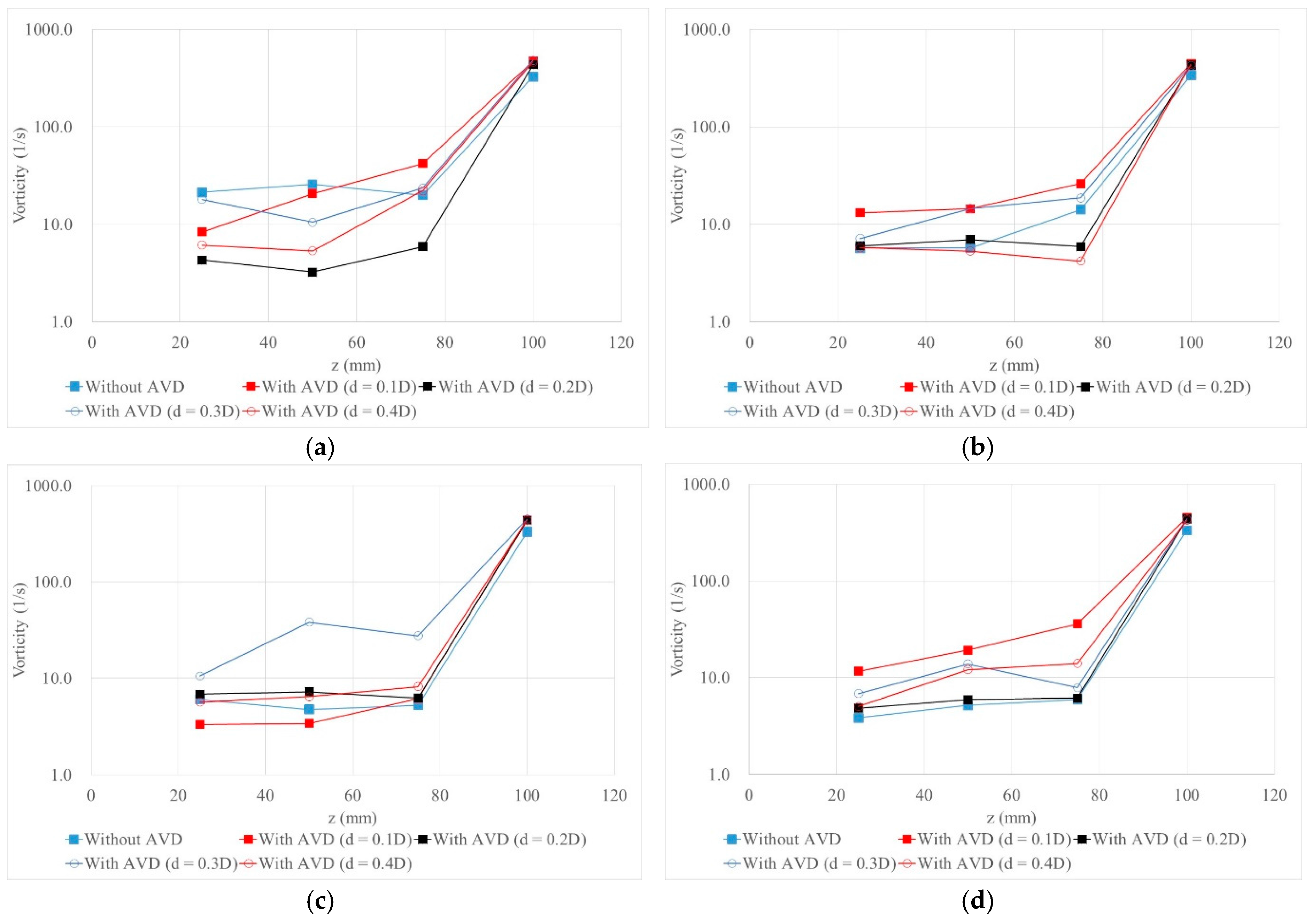
The main purpose of AVD installation is to decrease vorticity in a pump sump. Thus, the vorticity change analysis is the most important in AVD studies. The numerically-calculated vorticities on the four comparison lines were compared with test cases and are shown in Figure 12. Figure 12a depicts the resultant vorticity by each case and the decreased vorticities by AVD installation. In particular, the case of AVD height d = 0.2D derived the most effective vorticity decrease. However, increased vorticities were observed in the region above z = 75 mm. It is surmised that the reduced flow area may primarily affect this region as a y-directional velocity change results. Figure 12b shows the simulated results of vorticity for the inflow depth of H = 0.20 m. In cases with AVD height d = 0.2D and 0.4D, decreased vorticity is observed at the z = 75 mm comparison line and vorticity results similar to the calculated results without AVD installation are obtained. However, the increased vorticities were simulated with the cases of AVD height d = 0.1D and 0.3D. Figure 12c depicts the calculated vorticity results under the numerical cases with an inflow depth of H = 0.25 m. When the AVD with height d = 0.3D was adopted in the pump sump, severely increased vorticity results were obtained. In most cases, with other AVD height cases, it showed similar results with those of the channel-only test case. This result may imply that inappropriate AVD installation can worsen the flow characteristics with an unexpected vortex. Figure 12d shows the numerical results with an inflow depth of H = 0.30 m, which is the deepest condition. In all cases, the calculated vorticities were increased after the installation of AVD in the pump sump. Only in the case of AVD height d = 0.2D, the increase of vorticity showed negligible quantities. The greatest vorticity increase was found for the AVD height d = 0.1D case. It can be surmised that if the flow characteristics are sufficiently stable, AVD installation may worsen the flow conditions in a pump sump.

The velocity and vorticity changes in each direction along the comparison lines under the numerical test cases of various AVD installation heights were compared. Distinguishable velocity changes were observed in the x-directional velocity comparisons. This implies that the flow area reduction primarily affects the approach direction velocity. As the x-directional flow velocity changes, definite velocity changes are observed in the y-axis. Furthermore, unexpected velocity increases were observed in some cases. This implies that the appropriate AVD height has to be determined in the pump sump design procedure to satisfy varying flow conditions. As seen from the vorticity result comparisons, inappropriate AVD height can worsen flow characteristics in a pump sump. If the pump operation conditions require AVD installation, like with the inflow depth H = 0.15 m and H = 0.20 m cases, the AVD height should be 0.2D.

The results of this study are derived from the first-order numerical scheme for convective and diffusion flow calculations. If the higher-order scheme was applied to the regeneration of pump sump flow, different results about the vortex region and strength may be calculated. Furthermore, only the tetrahedron mesh system was applied in this study. The different mesh systems could derive different numerical results. Thus, additional study about different numerical and mesh systems for pump sumps should be followed to improve the applicability of the present study results. Thus, it seems that the present results are useful to describe the trend about the effectiveness of AVD installations.

4. Concluding Remarks

In this study, a numerical model was applied to analyze the change of flow characteristics, such as velocities and vorticity caused by the installation of an anti-vortex device in a pump sump. Twenty test cases were performed with various flow depths and AVD height conditions. The numerical results were compared to qualitative and quantitative methods. The results of the qualitative analysis showed that the AVD installation can improve the flow characteristic by reducing the vortex region in most cases. In the AVD height d = 0.1D case, it can be concluded that the installation of AVD can worsen the flow field in a pump sump. To analyze the numerical results more accurately, the velocity and vorticity variations along the chosen comparison lines were compared. According to the comparisons of the flow velocity results, it was found that the AVD installation cannot improve flow characteristics in all flow conditions. AVD installation is most effective for the low inflow depth conditions, which showed severe vortex regions in the uncontrolled case. If the flow in the pump sump was stable without AVD, AVD installation may worsen the flow field compared with that of the uncontrolled case. The numerical results comparison shows that the appropriate AVD height to improve flow characteristics by reducing vortices without a severe velocity increase may be 0.2D. Although these results were only derived in an experimental scale channel, it can be concluded that the suggested results can be considered in the design process of a pump station and can contribute to improving the performance of flood-control facilities.

References

1. Arboleda, G.; El-Fadel, M. Effects of Approach Flow Conditions on Pump Sump Design. J. Hydraul. Eng. 1996, 122, 489–494. [Google Scholar] [CrossRef]
2. Bauer, D.I.; Nakato, T. Subsurface Vortex Suppression in Water Intakes with Multiple-Pump Sumps; IIHR Report No. 389; Iowa Institute of Hydraulic Research, University of Iowa: Iowa City, IA, USA, 1997. [Google Scholar]
3. Constantinu, G.S.; Patel, V. Numerical Model for Simulation of Pump-intake Flow and Vortices. J. Hydraul. Eng. 1997, 124, 123–134. [Google Scholar] [CrossRef]
4. Rajendran, V.P.; Constantinescu, G.S.; Patel, V.C. Experiments on Flow in a Model Water-pump Intake Sump to Validate a Numerical Model. In Proceedings of the ASME Fluids Engineering Division Summer Meeting, Washington, DC, USA, 21–25 June 1998.
5. Rajendran, V.; Patel, V. Measurement of Vortices in Model Pump-Intake Bay by PIV. J. Hydraul. Eng. 2000, 126, 322–334. [Google Scholar] [CrossRef]
6. Nagahara, T.; Sato, T.; Okamura, T. Measurement of the Flow around the Submerged Vortex Cavitation in a Pump Intake by Means of PIV. In Proceedings of the 5th International Symposium on Cavitation, Osaka, Japan, 1–5 November 2003.
7. Choi, J.W. A Study on the Flow Characteristics around Intakes within a Sump in a Pump Station by PIV. Master’s Dissertation, Korea Maritime and Ocean University, Busan, Korea, 2003. [Google Scholar]
8. Turbomachinery Society of Japan. Standard Method for Model Testing the Performance of a Pump Sump; TSJ S002; TSJ: Tokyo, Japan, 2005. (In Japanese) [Google Scholar]
9. Johansson, A.E.; Stacy, P.S.; White, D.K.; Lin, F. Advancements in Hydraulic Modeling of Cooling Water Intakes in Power Plants. In Proceedings of the PWR2005 Conference, Chicago, IL, USA, 5–7 April 2005; pp. 7–16.
10. Okamura, T.; Kamemoto, K.; Matsui, J. CFD Prediction and Model Experiment on Suction Vortices in Pump Sump. In Proceedings of the 9th Asian Conference on Fluid Machinery, Jeju, Korea, 16–19 October 2007; pp. 1–10.
11. Park, S.E.; Roh, H.W. CFD Prediction on Vortex in Sump Intake at Pump Station. J. KSFM 2007, 10, 39–46. (In Korean) [Google Scholar] [CrossRef]
12. Kim, J.H.; Choi, Y.S.; Lee, K.Y. A Numerical Study on the Suction Performance of a Submerged Cargo Pump. J. KSFM 2008, 11, 18–23. (In Korean) [Google Scholar]
13. Choi, J.W.; Choi, Y.D.; Lim, W.S.; Lee, Y.H. Numerical Analysis on the Flow Uniformity in a Pump Sump Model with Multi-pump Intake. J. KSFM 2009, 12, 14–22. (In Korean) [Google Scholar]
14. Choi, J.W.; Park, N.S.; Kim, S.S.; Park, S.S.; Lee, Y.H. Study on Performance Analysis of Pump within Sump Model with AVD installation by CFD. J. KSWW 2012, 26, 463–469. (In Korean) [Google Scholar] [CrossRef]
15. Hydraulic Institute. Pump Intake Design; ANSI/HI 9.8-1998; Hydraulic Institute: Parsippany, NJ, USA, 1998. [Google Scholar]
16. Carregal-Ferreira, J.; Holzwarth, A.; Menter, F.; Esch, T.; Luu, A. Advanced CFD Analysis of Aerodynamics Using CFX; AEA Technology GmbH: Otterfing, Germany, 2002; pp. 1–14. [Google Scholar]
17. Bardina, J.E.; Huang, P.G.; Coakley, T.J. Turbulence Modeling Validation, Testing, and Development; NASA Technical Memorandum 110446; NASA: Washington, DC, USA, 1997.
18. Jiang, M.; Machiraju, R.; Thompson, D. Detection and visualization of vortices. In Visualization Handbook; Johnson, C., Hansen, C., Eds.; Academic Press: New York, NY, USA, 2004; pp. 287–301. [Google Scholar]
19. Levy, Y.; Degani, D.; Seginer, A. Graphical Visualization of Vortical Flows by Means of Helicity. AIAA J. 1990, 28, 1347–1352. [Google Scholar]
Figure 1. Schematic diagram of the experimental flume.
Sustainability 09 00285 g001
Figure 2. CFX results obtained in the present and previous research: (a) x-directional velocity results; (b) y-directional velocity results; (c) z-directional velocity results; and (d) vorticity results.
Sustainability 09 00285 g002
Figure 3. Anti-vortex devices used in the numerical simulation.
Sustainability 09 00285 g003
Figure 4. Computational domain and mesh for the numerical simulation: (a) flow domain of pump sump with AVD; and (b) numerical mesh near AVD.
Sustainability 09 00285 g004
Figure 5. Comparison of calculated vortex regions under inflow depth is 0.15 m with changes in AVD height: (a) without AVD; (b) AVD height d = 0.1D; (c) AVD height d = 0.2D; (d) AVD height d = 0.3D; and (e) AVD height d = 0.4D.
Sustainability 09 00285 g005
Figure 6. Comparison of calculated vortex regions under inflow depth is 0.20 m with changes in AVD height: (a) without AVD; (b) AVD height d = 0.1D; (c) AVD height d = 0.2D; (d) AVD height d = 0.3D; and (e) AVD height d = 0.4D.
Sustainability 09 00285 g006
Figure 7. Comparison of calculated vortex regions under inflow depth is 0.25 m with changes in AVD height: (a) without AVD; (b) AVD height d = 0.1D; (c) AVD height d = 0.2D; (d) AVD height d = 0.3D; and (e) AVD height d = 0.4D.
Sustainability 09 00285 g007aSustainability 09 00285 g007b
Figure 8. Comparison of calculated vortex regions under inflow depth is 0.30 m with changes in AVD height: (a) without AVD; (b) AVD height d = 0.1D; (c) AVD height d = 0.2D; (d) AVD height d = 0.3D; and (e) AVD height d = 0.4D.
Sustainability 09 00285 g008
Figure 9. Comparison of calculated x-directional velocities: (a) inflow depth H = 0.15 m; (b) inflow depth H = 0.20 m; (c) inflow depth H = 0.25 m; and (d) inflow depth H = 0.30 m.
Sustainability 09 00285 g009
Figure 10. Comparisons of calculated y-directional velocities: (a) inflow depth H = 0.15 m; (b) inflow depth H = 0.20 m; (c) inflow depth H = 0.25 m; and (d) inflow depth H = 0.30 m.
Sustainability 09 00285 g010
Figure 11. Comparison of calculated z-directional velocities: (a) inflow depth H = 0.15 m; (b) inflow depth H = 0.20 m; (c) inflow depth H = 0.25 m; and (d) inflow depth H = 0.30 m.
Sustainability 09 00285 g011
Figure 12. Comparison of calculated vorticities with changing inflow depths and AVD heights: (a) inflow depth H = 0.15 m; (b) inflow depth H = 0.20 m; (c) inflow depth H = 0.25 m; and (d) inflow depth H = 0.30 m
Sustainability 09 00285 g012