Article

A Hybrid Multiple-Criteria Decision-Making Approach for Photovoltaic Solar Plant Location Selection

1
Department of Technology Management, Chung Hua University, Hsinchu 300, Taiwan
2
Department of Industrial Engineering and Management, National Chin-Yi University of Technology, Taichung 411, Taiwan
*
Author to whom correspondence should be addressed.
Sustainability 2017, 9(2), 184; https://doi.org/10.3390/su9020184
Submission received: 9 November 2016 / Accepted: 18 January 2017 / Published: 27 January 2017

Abstract

:
Due to decaying fossil resource and increasing environmental consciousness, the demand of renewable energy resources is escalating these days. Photovoltaic solar energy is one of the most popular renewable energy resources in places where sunlight is abundant. The selection of a desirable location for constructing a photovoltaic solar plant is the first and one of the most important stages in the plant construction to provide a long-term energy production. In this paper, a comprehensive multiple-criteria decision-making model, which incorporates the interpretive structural modeling (ISM), fuzzy analytic network process (FANP) and VIKOR (VlseKriterijumska Optimizacija I Kompromisno Resenje in Serbian, meaning multi-criteria optimization and compromise solution), is proposed to select the most suitable photovoltaic solar plant location. The ISM is applied first to determine the interrelationships among the criteria and among the sub-criteria, and the results are used to construct a decision-making network. The FANP is applied next to solve the network and to calculate the importance weights of the sub-criteria. Finally, the VIKOR is adopted to determine the ranking of the photovoltaic solar plant locations. The proposed model is applied in a case study in evaluating photovoltaic solar plant locations in Taiwan. By applying the proposed model, decision makers can have a better thinking process and make more appropriate decisions justifiably.

1. Introduction

Climate changes and environmental pollution have caught the attention of many developing and developed counties to replace fossil fuel energy with renewable energy. After a certain kind of renewable energy is preferred and selected, a suitable plant location must be selected. In short, the renewable energy location selection problem is one of the most important tasks in developing renewable energy plants.
More and more scholars have contributed in developing models for solving the renewable energy location selection problem. Some recent works are reviewed here. Yeh and Huang [1] proposed a model to understand the importance of various factors in evaluating wind farm locations by integrating goal/question/metric (GQM) method, fuzzy decision-making trial and evaluation laboratory (DEMATEL), and analytic network process (ANP). The GQM method was applied to classify factors into different dimensions, and the DEMATEL was used to find the correlations among the dimensions. The ANP was then adopted to obtain the relative weights of the criteria. Kang et al. [2] constructed an approach by integrating the fuzzy ANP (FANP) and benefits-opportunities-costs-risks (BOCR) to facilitate the decision making of wind farm site selection. Tahri et al. [3] proposed the use of geographic information system (GIS) and analytic hierarchy process (AHP) to evaluate solar farm locations. The AHP was adopted to calculate the weights of four criteria: location, orography, land use and climate. The GIS was used to collect the data of these criteria in different locations. A case study was carried out to assess the suitability of a set of locations in southern Morocco. Chang [4] constructed a multi-choice goal programming model for devising an optimal mix of different renewable energy plant types in different locations while considering various criteria. The model could help decision makers determine appropriate weights to the factors, and find the optimal solution in the renewable energy capacity expansion planning problem. Lee et al. [5] constructed a two-stage framework for evaluating renewable energy plant site alternatives. In the first stage, fuzzy AHP (FAHP) was applied to set the assurance region (AR) of the quantitative factors. By incorporating the AR into data envelopment analysis (DEA), the efficiencies of a number of plant site candidates could be generated, and several sites were selected for further analysis. In the second stage, the FAHP was applied to select the most appropriate site by considering qualitative characteristics of the sites. Ribeiro et al. [6] studied the electric energy generation from small-scale solar and wind power, and listed three attributes, namely, location, area and shape, as having a great influence on power generation. A comparison method was applied in a case study in Brazil. Aragonés-Beltrán et al. [7] proposed two multiple-criteria decision-making models to evaluate photovoltaic solar power plant investment projects by considering six categories of risks and fifty project execution delay and/or stoppage risks. An AHP model, which considered the problem as a hierarchy, and an ANP model, which considered the problem as a network, were constructed to select the plant which minimized the overall risk. Sánchez-Lozano et al. [8] presented a framework, which integrated GIS, AHP and TOPSIS, to the optimal placement of photovoltaic solar power plants. GIS was applied to reduce the geographical area of study by considering constraints and weighting criteria. The weights of the criteria were calculated by the AHP, and the ranking of the power plants was obtained by applying the TOPSIS. Aragonés-Beltrán et al. [9] proposed a three-phase multi-criteria decision approach for selecting solar-thermal power plant investment projects. In the first phase, a project was accepted or rejected according to a set of criteria grouped as risks, costs and opportunities using an AHP model. In the second phase, the accepted projects were further assessed in risks using the AHP model. In the third phase, a ranking of the projects that were economically profitable based on project risk levels and execution time delays was prepared using both the AHP and the ANP models. Wu et al. [10] proposed a three-stage framework of solar thermal power plant site selection. In the first stage, potential feasible sites were identified based on energy, infrastructure, land, and environmental and social factors. In the second stage, the importance weights of the criteria were calculated by fuzzy measures. In the third stage, the sites were ranking using a group decision making method with linguistic Choquet integral (LCI). Sánchez-Lozano et al. [11] proposed a hybrid method to evaluate suitable locations for the installation of solar thermoelectric power plants. GIS was applied to limit the location alternatives, and the AHP was used to obtain the weights of the criteria. Then, the fuzzy TOPSIS was used to rank the alternatives.
A decision-making model is necessary for selecting the most suitable photovoltaic solar plant location. Therefore, this research incorporates three well-known methodologies, the interpretive structural modeling (ISM), the FANP and the VIKOR (VlseKriterijumska Optimizacija I Kompromisno Resenje in Serbian, meaning multi-criteria optimization and compromise solution), to facilitate the decision-making process. The rationale behind using the three different methodologies is to overcome the drawback of the FANP. While the ANP and the FANP have become rather popular multiple-criteria decision-making methodologies, a questionnaire is usually very lengthy if all the interrelationships among the criteria and among the sub-criteria are evaluated. In addition, the requirement of pairwise comparing the performance of each of the two alternatives with respect to each sub-criterion can be very tiresome for the person who fills out the questionnaire. Therefore, a model that integrates the ISM, the FANP and the VIKOR can overcome such problems. Since an evaluation network can be rather complex, the ISM is applied first to understand the interrelationships among the criteria and among the sub-criteria. Based on the interrelationships, the network can be constructed comprehensively. The FANP is then used to calculate the importance weights of the sub-criteria in the network. Based on the weights of the sub-criteria, the VIKOR is applied to calculate the overall performances of the photovoltaic solar plant locations.
The rest of this paper is organized as follows. In Section 2, the methodologies are briefly introduced. In Section 3, the proposed model, which incorporates the ISM, the FANP, and the VIKOR, is presented. In Section 4, a case study for selecting the most suitable photovoltaic solar plant location in Taiwan is presented. In the final section, some conclusion remarks are made.

2. Literature Review

In this section, the ISM, the FANP, and the VIKOR are briefly introduced, and some recent works are reviewed.

2.1. Interpretive Structural Modeling (ISM)

Interpretive structural modeling (ISM) was first proposed by Warfield to understand complex situations and to put together a course of action for tackling a problem [12,13,14]. Experts’ practical experience and knowledge are applied to decompose a complicated system into several subsystems (elements), and questions such as “Does criterion xi affect criterion xj?” are asked. A binary matrix, called relation matrix or adjacency matrix, is constructed first to present the relations of the elements [15]. By considering transitivity, a reachability matrix is prepared next. Finally, by applying the operators of the Boolean multiplication and addition, a final reachability matrix is calculated, and the matrix can reflect the convergence of the relationship among the elements.
Since its introduction, the ISM has been adopted in various fields. Some recent works are as follows. Rao et al. [16] constructed a schedule risk management framework for power grid engineering projects. The relationships among risks were determined by the ISM method first, and then a three-tier evaluation system was developed by the AHP. Shen et al. [17] performed a factor analysis on the implementation of an emission trading system in the Chinese building sector. The ISM method was adopted to establish a hierarchy structure between factors, and the MICMAC (matriced’ impacts croisés multiplication appliquée á un classement) technique was applied to analyze the driving-power and dependence power for each factor. Hussain et al. [18] constructed an evaluation framework for sustainable supply chain management alternatives. The ISM was applied to understand the relationships among different criteria, and the ANP was used to consider the correlated criteria when evaluating alternatives. Purohit et al. [19] studied enablers of mass customization for the Indian footwear units, and applied the ISM to understand the contextual relations among the enablers. The MICMAC analysis was used next to categorize the enablers.

2.2. Analytic Network Process (ANP)

Analytic network process (ANP), proposed by Saaty [20], is a multiple-criteria decision support methodology. It is a generalization of analytic hierarchy process (AHP), which was also introduced by Saaty [21]. The ANP replaces a hierarchy under the AHP with a network, in which the relationships between levels are not easily represented as higher or lower, dominated or being dominated, directly or indirectly [22]. The importance of all factors, including goal, criteria, sub-criteria and alternatives and the interrelationships among the factors are pairwise compared, and a supermatrix is constructed. A weighted supermatrix is calculated to ensure column stochastic [20]. By raising the weighted supermatrix to powers, a limit supermatrix is obtained to generate final solutions. Because uncertainty and ambiguity are often present in real-life problems, fuzzy set theory has been incorporated into the ANP, and the methodology is called fuzzy ANP, or FANP.
Some recent FANP works are reviewed below. Lee et al. [23] presented a conceptual model for product strategy evaluation in the photovoltaic silicon thin-film solar cell power industry by applying the ISM, the FANP and the BOCR. Lee et al. [24] proposed an integrated model, by adopting the ISM and the FANP, to understand the interrelationships among criteria and to evaluate different technologies for a flat panel manufacturer. Kang et al. [25] integrated the ISM, the BOCR and the FANP to evaluate the performances of wind farms. The ISM was used to determine the feedback and interdependency of the factors in a network with the BOCR aspects, and the FANP was applied to calculate the performance of the wind farms. Lee et al. [26] developed an evaluation model, by integrating the ISM and the FANP to help select suitable turbines in a wind farm. Wang et al. [27] presented a city sports center performance evaluation model by integrating the DEMATEL approach and the FANP. The DEMATEL was applied first to understand the importance and causal relationships among the evaluation factors of sports center based on the views of the managers. The FANP was used next to calculate the importance weights of the factors. Chen et al. [28] presented a hybrid multiple-criteria decision-making model by incorporating the ISM and the FANP to evaluate various strategies for new product development. Lu et al. [29] proposed a systematic method for developing effective sustainable improvement strategies to enhance competitive advantages. The method integrated the balanced scorecard, the DEMATEL, the ANP and the VIKOR.

2.3. VIKOR

The VIKOR is a multi-criteria decision-making technique developed by Opricovic [30] for optimizing complex systems. The methodology aims to rank and select the best or compromise solution from a set of alternatives. The best alternative is the one with the smallest distance to the positive ideal solution using three measures: aggregating index, group utility, and individual regret. A compromise solution, which is composed of more than one alternative, may be present if the conditions for single best alternative are not met [31].
The use of the VIKOR is also often found in solving multi-criteria decision-making problems. Tavana et al. [32] proposed a multiple-criteria decision-making model by integrating the VIKOR and the FAHP. The FAHP was applied to calculate the weights of the multiple criteria based on the linguistic judgments of different experts. Using the calculated criterion weights, the VIKOR was adopted to obtain a ranking of the alternatives based on these criteria which are stochastic. Safari et al. [33] proposed a methodology by combining failure mode and effect analysis (FMEA) and the fuzzy VIKOR for identifying and evaluating enterprise architecture risks. Instead of calculating the risk priority number (RPN) using the conventional FMEA, enterprise architecture risks were prioritized using the fuzzy VIKOR. Babashamsi et al. [34] prioritized pavement maintenance activities by proposing an integrated FAHP and VIKOR method. The FAHP was applied to calculate the weights of the performance indices, which were subsequently used to rank the activity alternatives by the VIKOR model. Li and Zhao [35] constructed a hybrid multiple-criteria decision-making framework using the VIKOR, the FAHP, and the grey relation analysis (GRA) to evaluate the performance of eco-industrial thermal power plants. The FAHP and Shannon entropy were applied to obtain the weights of the criteria, and the GRA was used to modify the conventional aggregating function of the VIKOR. Singh et al. [36] constructed an integrated AHP-VIKOR method under interval-valued fuzzy environment for sustainable manufacturing strategy selection, and linguistic variables were adopted to evaluate the performance of strategies and the weights of criteria. Mardani et al. [37] performed a systematic review of some papers published from 2003 to 2015 that applied multiple-criteria decision-making approaches in sustainable and renewable energy systems problems. The works were categorized into six groups: AHP and FAHP, ANP and VIKOR, technique for order of preference by similarity to ideal solution (TOPSIS) and fuzzy TOPSIS, preference ranking organization method for enrichment evaluations (PROMETHEE), integrated methods, and other methods. Mardani et al. [38] carried out a systematic review of the works published in 2004 to 2015 that applied the VIKOR method in areas such as sustainability and renewable energy.

3. Proposed Model

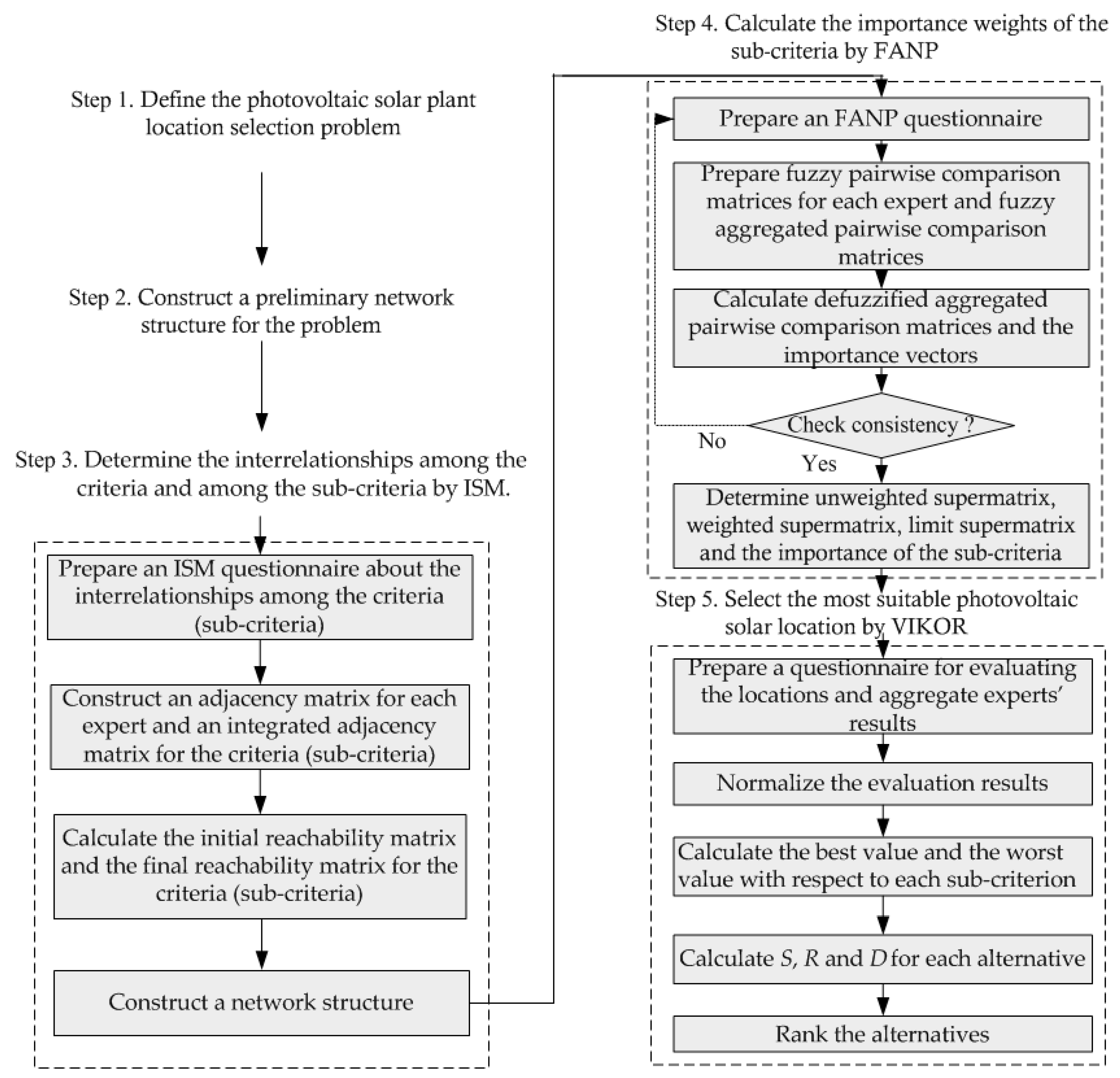
A model that incorporates the ISM, the FANP and the VIKOR is proposed here for the selection of the most suitable location for constructing a photovoltaic solar plant. The flowchart of the model is as depicted in Figure 1. The ISM is used to determine the interrelationships among the criteria and among the sub-criteria, and a network can be constructed based on the interrelationships. The FANP is adopted next to obtain the importance weights of the sub-criteria in the network. Using the weights of the sub-criteria from the FANP, the VIKOR is used to rank the overall performances of the photovoltaic solar plant locations.
The steps of the proposed model are as follows.
Step 1. Define the photovoltaic solar plant location selection problem. Perform a comprehensive literature review and consult experts in the field about the problem.
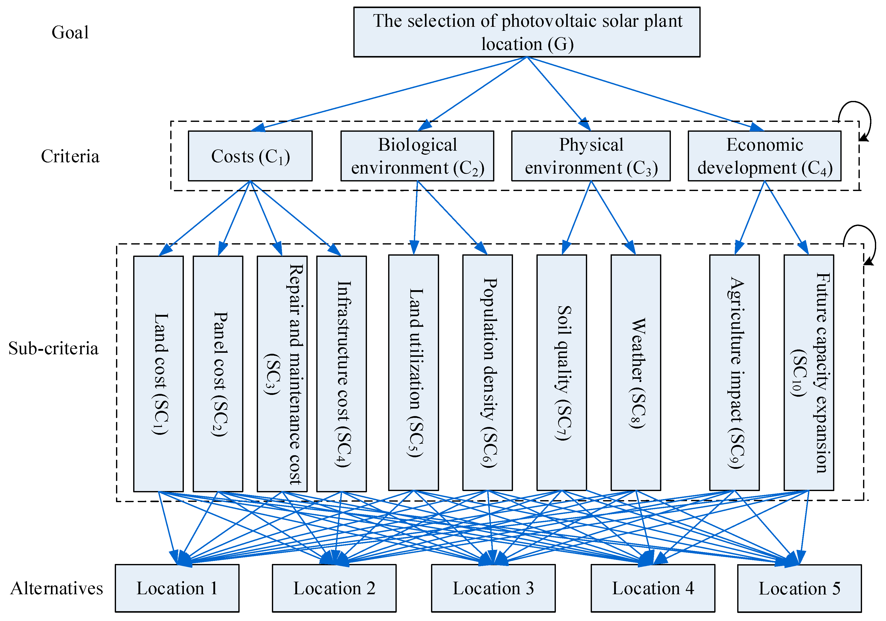
Step 2. Construct a preliminary network structure for the problem. Based on the literature and expert consultation, a network with criteria and sub-criteria is constructed. An example of the network is depicted in Figure 2, and the interrelationships among the criteria and among the sub-criteria will be determined by Step 3.
Step 3. Determine the interrelationships among the criteria and among the sub-criteria by applying the ISM.
Step 3.1. Prepare an ISM questionnaire. Based on the preliminary network, the ISM questionnaire asks about the interrelationships among the criteria and among the sub-criteria. For example, the relationship between criterion 1 and criterion 2 can be from C1 to C2, from C2 to C1, in both directions between C1 and C2, or C1 and C2 are unrelated.
Step 3.2. Construct an adjacency matrix for the criteria and for the sub-criteria from each expert. For example, the adjacency matrix for the criteria from expert k can be represented as follows:
A C k = C 1 C 2 C N C 1 C 2 C N [ 0 x 12 k x 1 N k x 21 k 0 x 2 N k 0 x N 1 k x N 2 k 0 ] ,   i = 1 , 2 , , N ;   j = 1 , 2 , , N
where x i j 1 denotes the relation between criteria Ci and Cj assessed by expert k, and x i j 1 = 1 if Cj is reachable from Ci; otherwise, x i j 1 = 0.
Step 3.3. Construct an integrated adjacency matrix for the criteria and for the sub-criteria. For example, the adjacency matrix for the criteria is prepared by combining the adjacency matrix for the criteria from all experts using the arithmetic mean method. If the calculated value for x i j is greater than or equal to 0.5, we let x i j be 1; otherwise, let x i j be 0. The integrated adjacency matrix for the criteria can be represented as follows:
A C = C 1 C 2 C N C 1 C 2 C N [ 0 x 12 x 1 N x 21 0 x 2 N 0 x N 1 x N 2 0 ] ,   i = 1 , 2 , , N ;   j = 1 , 2 , , N
where x i j denotes the relation between criteria Ci and Cj, and x i j = 1 if Cj is reachable from Ci; otherwise, x i j = 0.
Step 3.4. Calculate the initial reachability matrix for the criteria and for the sub-criteria. The initial reachability matrix can be obtained by summing up the integrated adjacency matrix and the unit matrix. For example, the initial reachability matrix for the criteria is as follows:
R C = A C + I
Step 3.5. Calculate the final reachability matrix. A convergence can be met by using the operators of the Boolean multiplication and addition. The final reachability matrix can reflect the transitivity of the contextual relation among the criteria and among the sub-criteria. For example, the final reachability matrix for the criteria is as follows:
R C * = R C l = R C l + 1 ,   l > 1
R C * = C 1 C 2 C N C 1 C 2 C N [ x 11 * x 12 * x 1 N * x 21 * x 22 * x 2 N * x i j * x N 1 * x N 2 * x N N * ] ,   i = 1 , 2 , , N ;   j = 1 , 2 , , N
where x i j * denotes the impact of criterion Ci to criterion Cj.
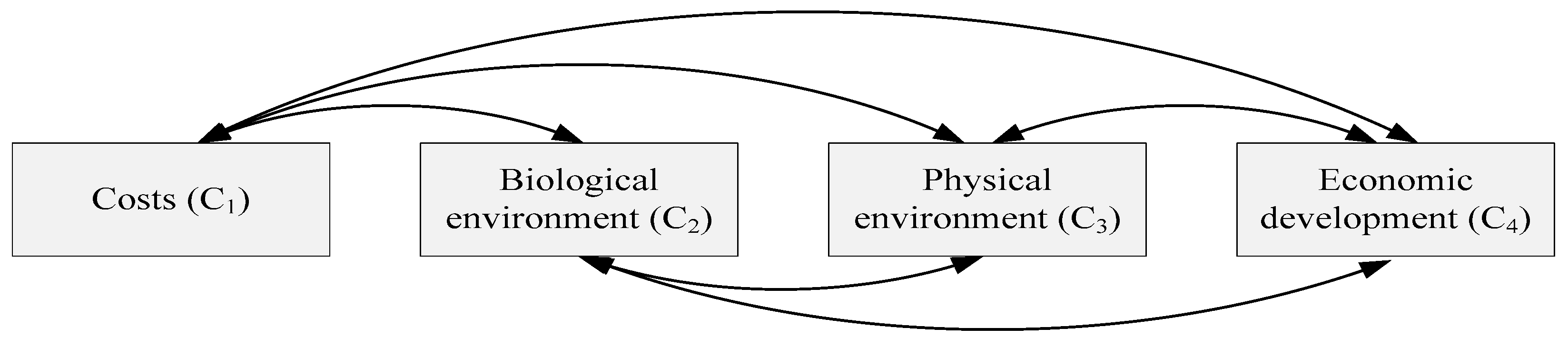
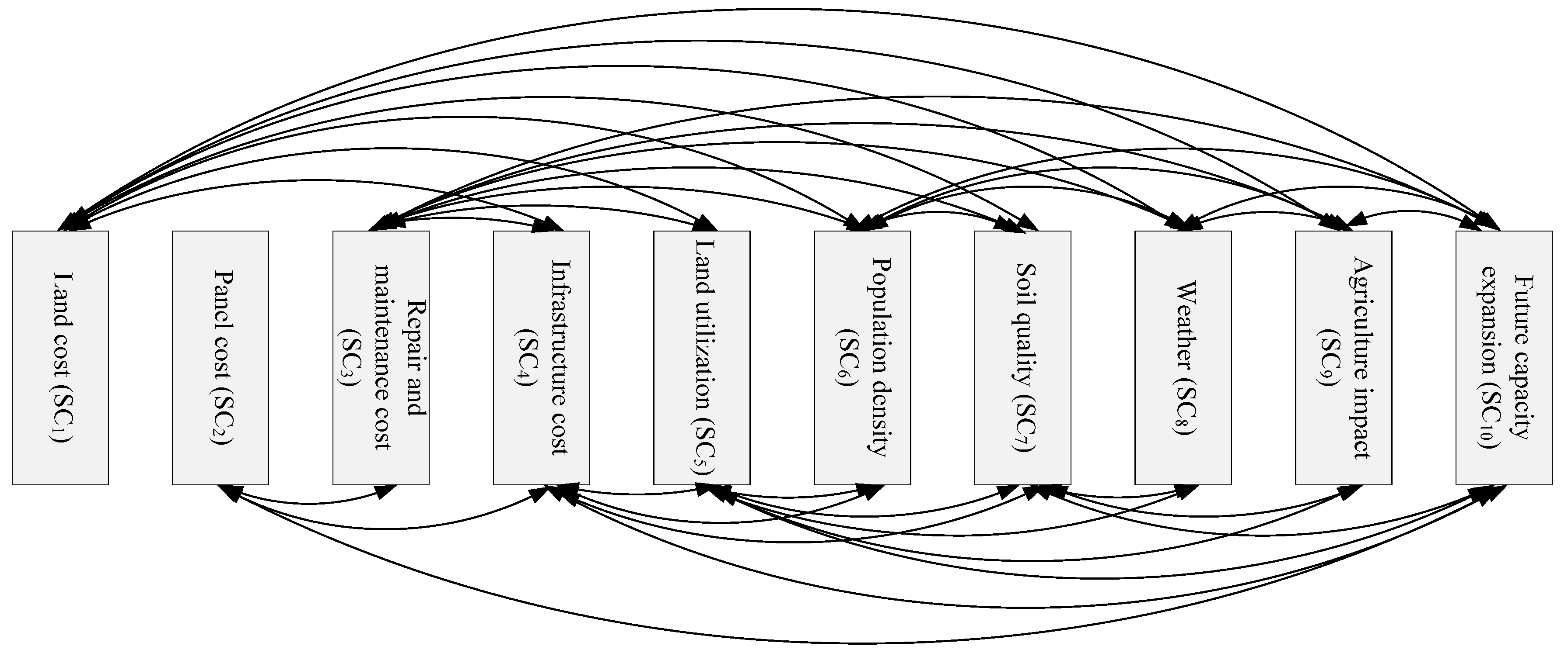
Step 3.6. Construct a network structure under the FANP. Based on the final reachability matrix for the criteria and for the sub-criteria, a completed network structure can be constructed.
Step 4. Calculate the importance weights of the sub-criteria by applying the FANP.
Step 4.1. Prepare an FANP questionnaire. Based on the network in Figure 2, the FANP questionnaire asks about the importance of the criteria, the importance of the sub-criteria, the interrelationships among the criteria, and the interrelationships among the sub-criteria. Experts in the field are invited to fill out the questionnaire using pairwise comparisons based on linguistic variables, as shown in Table 1.
Step 4.2. Prepare fuzzy pairwise comparison matrices for each expert. The questionnaire results from each expert are transformed into triangular fuzzy numbers based on Table 1. For example, the fuzzy pairwise comparison matrix of criteria for expert k is as follows:
W ˜ C k = C 1 C 2 C N C 1 C 2 C N [ 1 a ˜ 12 k a ˜ 1 N k a ˜ 21 k 1 a ˜ 2 N k a ˜ i j k a ˜ N 1 k a ˜ N 2 k 1 ] ,   i = 1 , 2 , , N ;   j = 1 , 2 , , N
where a ˜ i j k is the pairwise comparison value between criterion i and j determined by expert k.
Step 4.3. Prepare fuzzy aggregated pairwise comparison matrices. Synthesize experts’ opinions using a geometric average approach. With K experts, the geometric average for the pairwise comparison value between criteria i and j is:
f ˜ i j = ( a ˜ i j 1 a ˜ i j K ) 1 K = ( l i j , m i j , u i j ) ,   i = 1 , 2 , , N ;   j = 1 , 2 , , N
The fuzzy aggregated pairwise comparison matrix for the criteria is:
W ˜ C = C 1 C 2 C N C 1 C 2 C N [ 1 f ˜ 12 f ˜ 1 N f ˜ 21 1 f ˜ 2 N f ˜ i j f ˜ N 1 f ˜ N 2 1 ] ,   i = 1 , 2 , , N ;   j = 1 , 2 , , N
Step 4.4. Calculate defuzzified aggregated pairwise comparison matrices. The fuzzy aggregated pairwise comparison matrices are transformed into defuzzified aggregated pairwise comparison matrices using the center-of-gravity method.
f i j = l i j + m i j + u i j 3 ,   i = 1 , 2 , , N ;   j = 1 , 2 , , N
W C = C 1 C 2 C N C 1 C 2 C N [ 1 f 12 f 1 N 1 / f 12 1 f 2 N f i j 1 / f 1 N 1 / f 2 N 1 ] ,   i = 1 , 2 , , N ;   j = 1 , 2 , , N
Step 4.5. Calculate the importance vector of the criteria, importance vector of the sub-criteria, interdependence among the criteria, and interdependence among the sub-criteria. For example, the importance vector for the defuzzified aggregated pairwise comparison for the criteria is as follows [20,21]:
W C × w C = λ max × w C
where WC is the defuzzified aggregated comparison matrix for the criteria, wC is the eigenvector, and λ max is the largest eigenvalue of WC.
Step 4.6. Examine the consistency of each defuzzified aggregated pairwise comparison matrix. The consistency index (CI) and consistency ratio (CR) for the defuzzified aggregated comparison matrix for the criteria are calculated as follows [20,21]:
CI C = λ max N N 1
CR C = CI C RI
where RI is random index [20,21]. If the consistency ratio is greater than 0.1, an inconsistency is present, and the experts will be asked to revise the part of the questionnaire. The calculations will be performed again.
Step 4.7. Construct an unweighted supermatrix. Use the importance vector of the criteria, the importance vectors of the sub-criteria, the interdependence among criteria, and the interdependence among sub-criteria to form an unweighted supermatrix, as shown in Figure 3.
Step 4.8. Construct a weighted supermatrix. The unweighted supermatrix is transformed into a weighted supermatrix to ensure column stochastic [21,39].
Step 4.9. Calculate the limit supermatrix and the importance of the sub-criteria. By taking powers, the weighted supermatrix can converge into a stable supermatrix, called the limit supermatrix. The final priorities (importance) of the sub-criteria are found in the sub-criteria-to-goal column of the limit supermatrix.
Step 5. Select the most suitable photovoltaic solar location (alternative) by applying the VIKOR.
Step 5.1. Prepare a questionnaire for evaluating the expected performance of each photovoltaic solar location with respect to each sub-criterion. Experts in the field are invited to fill out the questionnaire with a scale from 1 to 10.
Step 5.2. Aggregate experts’ evaluation results. The evaluation results with respect to each sub-criterion from all experts are aggregated by using the arithmetic mean method.
Step 5.3. Normalize the evaluation results. For each sub-criterion, the experts’ aggregated evaluation results are normalized as follows:
Z p q = X p q / q = 1 Q X p q   , p = 1 ,   2 , , P ;   q = 1 ,   2 , , Q
where Z p q is the normalized evaluation result for alternative q with respect to sub-criterion p, X p q is the aggregated evaluation result for alternative q with respect to sub-criterion p, sub-criteria p = 1, 2, …, P, and alternative q = 1, 2, …, Q.
Step 5.4. Calculate the best value Z p * and the worst value Z p with respect to each sub-criterion p. For a sub-criterion that is a benefit, that is, the larger the better, the best value is the largest value among all values of the alternatives with respect to that sub-criterion. The worst value is the smallest value among all values of the alternatives with respect to that sub-criterion.
Z p * = max q Z p q ,   p = 1 ,   2 , , P
Z p = min q Z p q ,   p = 1 ,   2 ,   , P
The opposite is applied for a cost criterion:
Z p * = min q Z p q ,   p = 1 ,   2 ,   , P
Z p = max q Z p q ,   p = 1 ,   2 ,   , P
Step 5.5. Calculate group utility Sq and individual regret Rq for each alternative q.
S q = p = 1 P α p ( Z p * Z p q ) / ( Z p * Z p - ) ,   q = 1 ,   2 ,   , Q
R q = max p [ α p ( Z p * Z p q ) / ( Z p * Z p - ) ] ,   q = 1 ,   2 ,   , Q
where α p is the relative weights (importance) of sub-criteria obtained from Step 4.
Step 5.6. Calculate aggregating index Dq for each alternative q.
D q = v ( S q S * ) / ( S S * ) + ( 1 v ) ( R q R * ) / ( R R * ) ,   q = 1 ,   2 ,   , Q
where S * = min q S q , S = max q S q , R * = min q R q , R = max q R q , and v is the weight of the strategy of the majority of sub-criteria (here v = 0.5).
Step 5.7. Rank the alternatives. Three ranking lists are prepared based on Dq, Sq, Rq, respectively. The smaller the value of Dq an alternative has, the better the expected performance the alternative has. The same applies to Sq and Rq. The ranking for Dq is qD′, qD″, qD″′, etc. For example, qD′ is the best alternative in terms of Dq, and it has the smallest Dq, D′. The ranking for Sq is qS′, qS″, qS″′, etc., and their respective Sq are S′, S″, S″′, etc. The ranking for Rq is qR′, qR″, qR″′, etc., and their respective Rq are R′, R″, R″′, etc.
Step 5.8. Determine the best alternative. The best overall alternative is qD′ if the following two conditions are both met:
Condition 1.
Acceptable advantage:
D″ − D′ ≥ 1/(Q − 1)
where D′ is the value Dq for the best alternative (qD′) in terms of Dq, D″ is the value Dq for the second best alternative (qD″) in terms of Dq, and Q is the total number of alternatives. This condition implies that the difference between D′ and D″ is significant enough to indicate that the best alternative outperforms the second best alternative in terms of Dq.
Condition 2.
Acceptable stability in decision making: The best alternative in terms of Dq, that is, alternative qD′, must also be the best alternative in terms of both Sq and Rq. That is, qD′, qS′ and qR′ are the same alternative.
If the above two conditions are not satisfied, there are compromise solutions:
Situation 1.
Both alternative qD′ and qD″ are compromise solutions if only condition 2 is not met.
Situation 2.
Alternatives qD′, qD″, …, qD(H) are compromise solutions if condition 1 is not met. Alternative qD(H) is determined by
D(H)D′ < 1/(Q − 1)
This indicates that the performances of these alternatives are not significantly different, and as a result, they are compromise solutions.

4. Case Study

In this section, the proposed model is applied to a power company for selecting a suitable location for constructing a photovoltaic solar plant in Taiwan.

4.1. Define and Construct a Preliminary Network for the Photovoltaic Solar Plant Location Selection Problem

After an extensive literature review and interview with experts in the field, a preliminary network structure for the problem is constructed, as depicted in Figure 4. Under the goal of selecting the most suitable photovoltaic solar plant location, four criteria need to be considered, namely, costs (C1), biological environment (C2), physical environment (C3), and economic development (C4). Under costs (C1), there are four sub-criteria: land cost (SC1), panel cost (SC2), repair and maintenance cost (SC3), and infrastructure cost (SC4). Under biological environment (C2), there are two sub-criteria: land utilization (SC5) and population density (SC6). Under physical environment (C3), there are two sub-criteria: soil quality (SC7) and weather (SC8). Under economic development (C4), there are two sub-criteria: agriculture impact (SC9) and future capacity expansion (SC10). Five locations are being evaluated: location 1, location 2, location 3, location 4 and location 5. These five alternative locations are chosen because they are available lands that may be used for constructing photovoltaic solar plants currently. Due to the nature of the problem, experts are invited to contribute their expertise and fill out the questionnaires. In this case study, there are five experts, including two power company entrepreneurs, two scholars and one government officer. These five experts need to fill out three sets of questionnaires, i.e., the ISM questionnaire, the FANP questionnaire and the VIKOR questionnaire.

4.2. Determine the Interrelationships among the Criteria and among the Sub-Criteria

In order to understand the interrelationships among the criteria and among the sub-criteria, the ISM is applied. An ISM questionnaire is collected from the five experts, and an adjacency matrix for the criteria and an adjacency matrix for the sub-criteria are prepared based on the opinions from each expert. For example, the adjacency matrix for the criteria from expert 1 is as follows:
A C 1 = C 1 C 2 C 3 C 4 C 1 C 2 C 3 C 4 [ 0 1 1 1 1 0 1 1 1 1 0 1 1 1 1 0 ]
The adjacency matrix for the sub-criteria from expert 1 is as follows:
Sustainability 09 00184 i001
Next, an integrated adjacency matrix for the criteria and an integrated adjacency matrix for the sub-criteria are calculated, as follows:
A C = C 1 C 2 C 3 C 4 C 1 C 2 C 3 C 4 [ 0 1 1 1 1 0 1 1 1 1 0 1 1 1 1 0 ]
Sustainability 09 00184 i002
Based on the integrated adjacency matrix for the criteria, the initial reachability matrix and the final reachability matrix for the criteria are calculated as follows:
R C = A C + I
= C 1 C 2 C 3 C 4 C 1 C 2 C 3 C 4 [ 0 1 1 1 1 0 1 1 1 1 0 1 1 1 1 0 ] + C 1 C 2 C 3 C 4 C 1 C 2 C 3 C 4 [ 1 0 0 0 0 1 0 0 0 0 1 0 0 0 0 1 ] = C 1 C 2 C 3 C 4 C 1 C 2 C 3 C 4 [ 1 1 1 1 1 1 1 1 1 1 1 1 1 1 1 1 ] R C * = R C 1 = R C 2 = C 1 C 2 C 3 C 4 C 1 C 2 C 3 C 4 [ 1 1 1 1 1 1 1 1 1 1 1 1 1 1 1 1 ]
Based on the integrated adjacency matrix for the sub-criteria, the initial reachability matrix and the final reachability matrix for the sub-criteria are calculated as follows:
R SC = A SC + I
Sustainability 09 00184 i003
Sustainability 09 00184 i004
Based on the final reachability matrix for the criteria and the final reachability matrix for the sub-criteria, the interrelationships among the criteria and among the sub-criteria are determined, as shown in Figure 5 and Figure 6.

4.3. Calculate the Importance Weights of the Sub-Criteria

The importance weights of the sub-criteria are calculated by applying the FANP. Based on Figure 4, Figure 5 and Figure 6, an FANP questionnaire is prepared and given out to the five experts. An example of the questionnaire is as shown in Table 2.
Based on the questionnaire feedback, fuzzy pairwise comparison matrices for each expert are prepared. For example, the fuzzy pairwise comparison matrix of criteria for expert 1 is:
Sustainability 09 00184 i005
Fuzzy aggregated pairwise comparison matrices are prepared by synthesizing the experts’ opinions using a geometric average approach. The fuzzy aggregated pairwise comparison matrix for the criteria is:
Sustainability 09 00184 i006
Defuzzified aggregated pairwise comparison matrices are calculated next using the center-of-gravity method, and subsequently, the importance vectors of the criteria, the importance vectors of the sub-criteria, the interdependence among criteria, and the interdependence among sub-criteria can be obtained. For example, the defuzzified aggregated pairwise comparison matrix and the importance vector of the criteria are calculated, and the consistency test is performed:
W C = C 1 C 2 C 3 C 4 C 1 C 2 C 3 C 4 [ 1 3.21 1.63 5.47 0.31 1 0.41 2.88 0.61 2.45 1 5.21 0.18 0.35 0.2 1 ]
w C = [ 0.45472 0.15280 0.32695 0.06553 ] T C I C = λ max N N 1 = 4.0384 4 4 1 = 0.0128 C R C = C I C RI = 0.0128 0.9 = 0.0142
After the importance vector of the criteria, the importance vectors of the sub-criteria, the interdependence among the criteria, and the interdependence among the sub-criteria are calculated, an unweighted supermatrix is formed, as shown in Table 3. The weighted supermatrix and the limit supermatrix are also calculated, as shown in Table 4 and Table 5, respectively. The importance weights of the sub-criteria are found in the sub-criteria-to-goal column of the limit supermatrix in Table 5.
w SC = [ 0.14302 0.0799 0.10486 0.09315 0.16661 0.09587 0.10731 0.05948 0.0697 0.0801 ] T
Based on the case study, we can see that the experts stress the most on the costs (C1) criterion with an importance weight of 0.45472, followed by physical environment (C3) with an importance weight of 0.32695. For the sub-criteria, land utilization (SC5) is the most important with an importance weight of 0.16661, followed by land cost (SC1) with an importance weight of 0.14302. The third and fourth important sub-criteria are soil quality (SC7) with an importance weight of 0.10731 and repair and maintenance cost (SC3) with an importance weight of 0.10486, respectively.

4.4. Select the Most Suitable Photovoltaic Solar Location

The expected performances of the photovoltaic solar locations are evaluated through the VIKOR. A questionnaire for evaluating the expected performance of each photovoltaic solar location with respect to each sub-criterion is prepared, and the five experts are invited to contribute their expertise again. Arithmetic mean method is applied to aggregate the opinions of the experts, and the aggregated evaluation results are normalized, as shown in Table 6. The best value Z p * and the worst value Z p with respect to each sub-criterion p are calculated, as shown in Table 7. The values Sq, Rq and Dq for each alternative q are calculated next, as shown in Table 8. By applying Equation (19), we can obtain each Sq. For example, S1 is calculated as follows:
S1 = 0.14302 × (0.0629 − 0.1621)/(0.0629 − 0.314) + 0.07990 × (0.1770 − 0.2062)/(0.1770 − 0.215) + … + 0.08010 × (0.3236 − 0.1211)/(0.3236 − 0.1211) = 0.0565 + 0.0614 + … + 0.0801 = 0.4829
By applying Equation (20), we can obtain each Rq. For example, R1 is calculated as follows:
R1 = max[0.0565, 0.0614, …, 0.0801] = 0.0801
Table 8 shows that S* = 0.2044, S = 0.6963, R* = 0.0596 and R = 0.1666. By applying Equation (21), we can obtain each Dq. For example, D1 is calculated as follows:
D1 = 0.5 × (0.4829 − 0.2044)/(0.6963-0.2044) + (1 − 0.5) × (0.0801 − 0.0596)/(0.1666 − 0.0596) = 0.3790
Based on the aggregating index (Dq), location 2 ranks first, followed by location 3 and location 1. Based on the group utility (Sq), location 2 also ranks first, followed by location 3 and location 1. Based on the individual regret (Rq), location 2 again ranks first. However, location 1 ranks second, followed by location 3.
Based on Condition 1 in Step 5.8, Equation (22) must be examined. With D′ = 0, D″ = 0.3505 and Q = 5, we obtain:
D″ − D′ ≥ 1/(Q − 1)
0.3505 − 0 ≥ 1/(5 − 1) = 0.25
Thus, Condition 1 is passed. That is, in terms of Dq, location 2 outperforms location 3, the location with the second best Dq. Since location 2 is the best alternative in terms of both Sq and Rq, Condition 2 also passed. Therefore, we can conclude that location 2 is the most suitable for setting up the photovoltaic solar plant.

5. Conclusions

In this research, a comprehensive multiple-criteria decision-making model is proposed by incorporating the ISM, the FANP and the VIKOR. The model applies the ISM to understand the interrelationships among the criteria and among the sub-criteria, and then uses the FANP to calculate the importance weights of the sub-criteria. Finally, the VIKOR is adopted to select the most suitable photovoltaic solar plant location. A case study in Taiwan is used to demonstrate how the model can be implemented in real practice. By integrating the three methodologies, the major shortcoming of the FANP can be solved. That is, the length of the questionnaire can be reduced substantially. The proposed model can provide decision makers a better thinking process so that they can make appropriate decisions systematically.
Based on the case study, some results are found. Among the four criteria, the most important criterion is costs, followed by physical environment. Among the ten sub-criteria, land utilization is the most important sub-criterion, followed by land cost, soil quality, and repair and maintenance cost. The evaluation of the five locations shows that location 2 outperforms others in terms of both group utility and individual regret. Location 2 also performs the best on the aggregating index, which comprises both group utility and individual regret. In consequence, location 2 should be selected for constructing the photovoltaic solar plant.
The proposed model can be adopted by practitioners in relevant decision makings. The criteria or sub-criteria can be tailored according to the circumstances of the problem, and the experts in the field can contribute their expertise in determining the relative importance of and interrelationships among the factors. The expected performances of the alternatives can either be quantitative or qualitative, and the overall ranking of the alternatives can be obtained through the model.
In the case that many potential locations are available, a screening phase may be necessary to determine the feasible locations first. An extensive study of the feasible locations will then be carried out using the proposed approach. The screening phase can be performed using some tools, such as geographical information systems (GIS) or data envelopment analysis (DEA). This can be our future research direction.

Acknowledgments

This work was supported in part by the Ministry of Science and Technology in Taiwan under Grant MOST 105-2221-E-216-014-MY2.

Author Contributions

Amy H. I. Lee conceived the research, and drafted, edited, and revised the manuscript. He-Yau Kang designed the research, developed the model, and analyzed the data. You-Jyun Liou collected the data.

Conflicts of Interest

The authors declare no conflict of interest.

References

  1. Yeh, T.M.; Huang, Y.L. Factors in determining wind farm location: Integrating GQM, fuzzy DEMATEL, and ANP. Renew. Energy 2014, 66, 159–169. [Google Scholar] [CrossRef]
  2. Kang, M.S.; Chen, C.S.; Ke, Y.L.; Lee, A.H.I.; Ku, T.T.; Kang, H.Y. Applications of FANP and BOCR in renewable energy—Study on the choice of the sites for wind farms. IEEE Trans. Ind. Appl. 2013, 49, 982–989. [Google Scholar] [CrossRef]
  3. Tahri, M.; Hakdaoui, M.; Maanan, M. The evaluation of solar farm locations applying geographic information system and multi-criteria decision-making methods: Case study in southern Morocco. Renew. Sustain. Energy Rev. 2015, 51, 1354–1362. [Google Scholar] [CrossRef]
  4. Chang, C.T. Multi-choice goal programming model for the optimal location of renewable energy facilities. Renew. Sustain. Energy Rev. 2015, 41, 379–389. [Google Scholar] [CrossRef]
  5. Lee, A.H.I.; Kang, H.Y.; Lin, C.Y.; Shen, K.C. An integrated decision-making model for location of a PV solar plant. Sustainability 2015, 7, 13522–13541. [Google Scholar] [CrossRef]
  6. Ribeiro, A.E.D.; Arouca, M.C.; Coelho, D.M. Electric energy generation from small-scale solar and wind power in Brazil: The influence of location, area and shape. Renew. Energy 2016, 85, 554–563. [Google Scholar] [CrossRef]
  7. Aragonés-Beltrán, P.; Chaparro-González, F.; Pastor-Ferrando, J.P.; Rodríguez-Pozo, F. An ANP-based approach for the selection of photovoltaic solar power plant investment projects. Renew. Sustain. Energy Rev. 2010, 14, 249–264. [Google Scholar] [CrossRef]
  8. Sánchez-Lozano, J.M.; Teruel-Solano, J.; Soto-Elvira, P.L.; García-Cascales, M.S. Geographical Information Systems (GIS) and Multi-Criteria Decision Making (MCDM) methods for the evaluation of solar farms locations: Case study in south-eastern Spain. Renew. Sustain. Energy Rev. 2013, 24, 544–556. [Google Scholar] [CrossRef]
  9. Aragonés-Beltrán, P.; Chaparro-González, F.; Pastor-Ferrando, J.P.; Pla-Rubio, A. An AHP (Analytic Hierarchy Process)/ANP (Analytic Network Process)-based multi-criteria decision approach for the selection of solar-thermal power plant investment projects. Energy 2014, 66, 222–238. [Google Scholar] [CrossRef]
  10. Wu, Y.; Geng, S.; Zhang, H.; Gao, M.; China, N. Decision framework of solar thermal power plant site selection based on linguistic Choquet operator. Appl. Energy 2014, 136, 303–311. [Google Scholar] [CrossRef]
  11. Sanchez-Lozano, J.M.; Garcia-Cascales, M.S.; Lamata, M.T. Evaluation of suitable locations for the installation of solar thermoelectric power plants. Comput. Ind. Eng. 2015, 87, 343–355. [Google Scholar] [CrossRef]
  12. Warfield, J.N. Developing interconnected matrices in structural modeling. IEEE Trans. Syst. Man Cybern. 1974, 4, 51–81. [Google Scholar]
  13. Warfield, J.N. Toward interpretation of complex structural modeling. IEEE Trans. Syst. Man Cybern. 1974, 4, 405–417. [Google Scholar] [CrossRef]
  14. Warfield, J.N. Societal Systems: Planning, Policy and Complexity; John Wiley & Sons: New York, NY, USA, 1976. [Google Scholar]
  15. Huang, J.J.; Tzeng, G.H.; Ong, C.S. Multidimensional data in multidimensional scaling using the analytic network process. Pattern Recogn. Lett. 2005, 26, 755–767. [Google Scholar] [CrossRef]
  16. Rao, R.; Zhang, X.; Shi, Z.; Luo, K.; Tan, Z.; Feng, Y. A systematical framework of schedule risk management for power grid engineering projects’ sustainable development. Sustainability 2014, 6, 6872–6901. [Google Scholar] [CrossRef]
  17. Shen, L.; Song, X.; Wu, Y.; Liao, S.; Zhang, X. Interpretive structural modeling based factor analysis on the implementation of emission trading system in the Chinese building sector. J. Clean. Prod. 2016, 127, 214–227. [Google Scholar] [CrossRef]
  18. Hussain, M.; Awasthi, A.; Tiwari, M.K. Interpretive structural modeling-analytic network process integrated framework for evaluating sustainable supply chain management alternatives. Appl. Math. Model. 2016, 40, 3671–3687. [Google Scholar] [CrossRef]
  19. Purohit, J.K.; Mittal, M.L.; Mittal, S.; Sharma, M.K. Interpretive structural modeling-based framework for mass customisation enablers: An Indian footwear case. Prod. Plan. Control 2016, 27, 774–786. [Google Scholar] [CrossRef]
  20. Saaty, T.L. Decision Making with Dependence and Feedback: The Analytic Network Process; RWS Publications: Pittsburgh, PA, USA, 1996. [Google Scholar]
  21. Saaty, T.L. The Analytic Hierarchy Process; McGraw-Hill: New York, NY, USA, 1980. [Google Scholar]
  22. Meade, L.M.; Sarkis, J. Analyzing organizational project alternatives for agile manufacturing processes: An analytical network approach. Int. J. Prod. Res. 1999, 37, 241–261. [Google Scholar] [CrossRef]
  23. Lee, A.H.I.; Chen, H.H.; Kang, H.Y. A model to analyze strategic products for photovoltaic silicon thin-film solar cell power industry. Renew. Sustain. Energy Rev. 2011, 15, 1271–1283. [Google Scholar] [CrossRef]
  24. Lee, A.H.I.; Kang, H.Y.; Chang, C.C. An integrated ISM-FANP-BOCR model for selecting technologies. Int. J. Inform. Technol. Decis. Mak. 2011, 10, 843. [Google Scholar] [CrossRef]
  25. Kang, H.Y.; Hung, M.C.; Pearn, W.L.; Lee, A.H.I.; Kang, M.S. An integrated multi-criteria decision making model for evaluating wind farm performance. Energies 2011, 4, 2002–2026. [Google Scholar] [CrossRef]
  26. Lee, A.H.I.; Hung, M.C.; Kang, H.Y.; Pearn, W.L. A wind turbine evaluation model under a multi-criteria decision making environment. Energy Convers. Manag. 2012, 64, 289–300. [Google Scholar] [CrossRef]
  27. Wang, C.Y.; Tsai, P.H.; Zheng, H. Constructing Taipei City sports centre performance evaluation model with fuzzy MCDM approach based on views of managers. Math. Probl. Eng. 2013, 2013, 138546. [Google Scholar] [CrossRef]
  28. Chen, W.C.; Wang, L.Y.; Lin, M.C. A hybrid MCDM model for new product development: Applied on the Taiwanese LiFePO4 industry. Math. Probl. Eng. 2015, 2015, 462929. [Google Scholar] [CrossRef]
  29. Lu, I.Y.; Kuo, T.; Lin, T.S.; Tzeng, G.H.; Huang, S.L. Multicriteria decision analysis to develop effective sustainable development strategies for enhancing competitive advantages: Case of the TFT-LCD industry in Taiwan. Sustainability 2016, 8, 1–31. [Google Scholar] [CrossRef]
  30. Opricovic, S. Multicriteria Optimization of Civil Engineering Systems; Faculty of Civil Engineering: Belgrade, MT, USA, 1998. [Google Scholar]
  31. Opricovic, S.; Tzeng, G.H. Extended VIKOR method in comparison with outranking methods. Eur. J. Oper. Res. 2007, 178, 514–529. [Google Scholar] [CrossRef]
  32. Tavana, M.; Mavi, R.K.; Santos-Arteaga, F.J.; Doust, E.R. An extended VIKOR method using stochastic data and subjective Judgments. Comput. Ind. Eng. 2016, 97, 240–247. [Google Scholar] [CrossRef]
  33. Safari, H.; Faraji, Z.; Majidian, S. Identifying and evaluating enterprise architecture risks using FMEA and fuzzy VIKOR. J. Intell. Manuf. 2016, 27, 475–486. [Google Scholar] [CrossRef]
  34. Babashamsi, P.; Golzadfar, A.; Yusoff, N.I.M.; Ceylan, H.; Nor, N.G.M. Integrated fuzzy analytic hierarchy process and VIKOR method in the prioritization of pavement maintenance activities. Int. J. Pavement Res. Technol. 2016, 9, 112–120. [Google Scholar] [CrossRef]
  35. Li, N.; Zhao, H. Performance evaluation of eco-industrial thermal power plants by using fuzzy GRA-VIKOR and combination weighting techniques. J. Clean. Prod. 2016, 135, 169–183. [Google Scholar] [CrossRef]
  36. Singh, S.; Olugu, E.U.; Musa, S.N.; Mahat, A.B.; Wong, K.Y. Strategy selection for sustainable manufacturing with integrated AHP-VIKOR method under interval-valued fuzzy environment. Int. J. Adv. Manuf. Technol. 2016, 84, 547–563. [Google Scholar] [CrossRef]
  37. Mardani, A.; Jusoh, A.; Zavadskas, E.K.; Cavallaro, F.; Khalifah, Z. Sustainable and renewable energy: An overview of the application of multiple criteria decision making techniques and approaches. Sustainability 2015, 7, 13947–13984. [Google Scholar] [CrossRef]
  38. Mardani, A.; Zavadskas, E.K.; Govindan, K.; Senin, A.A.; Jusoh, A. VIKOR technique: A systematic review of the state of the art literature on methodologies and applications. Sustainability 2016, 8, 37. [Google Scholar] [CrossRef] [Green Version]
  39. Lee, A.H.I.; Chen, H.H.; Tong, Y. Developing new products in a network with efficiency and innovation. Int. J. Prod. Res. 2008, 48, 4687–4707. [Google Scholar] [CrossRef]
Figure 1. Flowchart of the model.
Sustainability 09 00184 g001
Figure 2. A network structure.
Sustainability 09 00184 g002
Figure 3. Unweighted supermatrix.
Sustainability 09 00184 g003
Figure 4. Network for the photovoltaic solar plant location selection.
Sustainability 09 00184 g004
Figure 5. Interrelationships among the criteria.
Sustainability 09 00184 g005
Figure 6. Interrelationships among the sub-criteria.
Sustainability 09 00184 g006
Table 1. Fuzzy numbers for relative importance.
Fuzzy NumberLinguistic VariableTriangular Fuzzy Number
1 ˜ Equally important(1, 1, 1)
3 ˜ Moderately important(1, 3, 5)
5 ˜ Important(3, 5, 7)
7 ˜ Very important(5, 7, 9)
9 ˜ Extremely important(9, 9, 9)
Table 2. FANP questionnaire.
For Selection of Photovoltaic Solar Plant Location (G), Which Criterion Is More Important?
Extremely importantVery importantImportantModerately importantEqually importantModerately importantImportantVery importantExtremely important
Costs (C1)Biological environment (C2)
Physical environment (C3)
Economic development (C4)
Under the Criterion Costs (C1), Which Sub-Criterion Is More Important?
Extremely importantVery importantImportantModerately importantEqually importantModerately importantImportantVery importantExtremely important
Land cost (SC1)Panel cost (SC2)
Repair and maintenance cost (SC3)
Infrastructure cost (SC4)
Table 3. Unweighted supermatrix.
GoalC1C2C3C4SC1SC2SC3SC4SC5SC6SC7SC8SC9SC10
Goal100000000000000
C10.454720.533460.26480.266540.247720000000000
C20.152800.130180.564950.124910.082480000000000
C30.326950.277790.11860.555420.173760000000000
C40.065530.058570.051660.053130.496030000000000
SC100.581760000.11386000.234640.24070.192860.178770.135790.103520.14744
SC200.2514700000.517270.164350.1373000000.10673
SC300.1124300000.193450.130040.141890.080470.116030.073490.228080.107480.11331
SC400.054330000.111580.127350.129020.089030.095220.098180.10037000.1142
SC5000.74253000.3368200.082730.119840.183250.094760.243920.148820.262360.07082
SC6000.25747000.0770500.148890.110230.076740.084690.104510.142140.131620.11513
SC70000.1254200.2173100.107160.089970.110870.075980.085920.083430.131680.09366
SC80000.8745800.0471100.0549100.090890.069130.050960.086780.121130.07661
SC900000.836560.0521400.0912800.061570.179560.07330.065180.06150.11446
SC1000000.163440.044140.161930.091620.077110.060290.088820.088750.109770.080710.04766
Table 4. Weighted supermatrix.
GoalC1C2C3C4SC1SC2SC3SC4SC5SC6SC7SC8SC9SC10
Goal0.500000000000000
C10.227360.266730.13240.133270.123860000000000
C20.076400.065090.282470.062460.041240000000000
C30.163480.138890.05930.277710.086880000000000
C40.032770.029290.025830.026560.248020000000000
SC100.290880000.11386000.234640.24070.192860.178770.135790.103520.14744
SC200.1257400000.517270.164350.1373000000.10673
SC300.0562200000.193450.130040.141890.080470.116030.073490.228080.107480.11331
SC400.027170000.111580.127350.129020.089030.095220.098180.10037000.1142
SC5000.37127000.3368200.082730.119840.183250.094760.243920.148820.262360.07082
SC6000.12873000.0770500.148890.110230.076740.084690.104510.142140.131620.11513
SC70000.0627100.2173100.107160.089970.110870.075980.085920.083430.131680.09366
SC80000.4372900.0471100.0549100.090890.069130.050960.086780.121130.07661
SC900000.418280.0521400.0912800.061570.179560.07330.065180.06150.11446
SC1000000.081720.044140.161930.091620.077110.060290.088820.088750.109770.080710.04766
Table 5. Limit supermatrix.
GoalC1C2C3C4SC1SC2SC3SC4SC5SC6SC7SC8SC9SC10
Goal000000000000000
C1000000000000000
C2000000000000000
C3000000000000000
C4000000000000000
SC10.143020.143020.143020.143020.143020.143020.143020.143020.143020.143020.143020.143020.143020.143020.14302
SC20.07990.07990.07990.07990.07990.07990.07990.07990.07990.07990.07990.07990.07990.07990.0799
SC30.104860.104860.104860.104860.104860.104860.104860.104860.104860.104860.104860.104860.104860.104860.10486
SC40.093150.093150.093150.093150.093150.093150.093150.093150.093150.093150.093150.093150.093150.093150.09315
SC50.166610.166610.166610.166610.166610.166610.166610.166610.166610.166610.166610.166610.166610.166610.16661
SC60.095870.095870.095870.095870.095870.095870.095870.095870.095870.095870.095870.095870.095870.095870.09587
SC70.107310.107310.107310.107310.107310.107310.107310.107310.107310.107310.107310.107310.107310.107310.10731
SC80.059480.059480.059480.059480.059480.059480.059480.059480.059480.059480.059480.059480.059480.059480.05948
SC90.06970.06970.06970.06970.06970.06970.06970.06970.06970.06970.06970.06970.06970.06970.0697
SC100.08010.08010.08010.08010.08010.08010.08010.08010.08010.08010.08010.08010.08010.08010.0801
Table 6. Normalized evaluation results of photovoltaic solar locations.
PrioritiesLocation (q = 1)Location (q = 2)Location (q = 3)Location (q = 4)Location (q = 5)
SC10.143020.16210.06290.21570.31400.2453
SC20.079900.20620.19650.20530.21500.1770
SC30.104860.19430.07770.24070.39220.0950
SC40.093150.20040.18970.19490.20550.2095
SC50.166610.26240.19870.23680.22030.0817
SC60.095870.19120.06880.20980.27040.2598
SC70.107310.18930.48390.13930.01050.1770
SC80.059480.22890.21140.22560.23100.1031
SC90.069700.35920.21300.17190.05660.1994
SC100.080100.12110.17300.32360.19190.1903
Table 7. Best values and worst values for each sub-criterion.
Best Value ( Z p * )Worst Value ( Z p )
SC10.06290.3140
SC20.17700.2150
SC30.07770.3922
SC40.18970.2095
SC50.26240.0817
SC60.06880.2704
SC70.48390.0105
SC80.23100.1031
SC90.05660.3592
SC100.32360.1211
Table 8. Ranking by Sq, Rq and Dq.
Location (q = 1)Location (q = 2)Location (q = 3)Location (q = 4)Location (q = 5)
Group utility (Sq)0.48290.20440.42320.69630.6750
Ranking by Sq31254
Individual regret (Rq)0.08010.05960.08700.14300.1666
Ranking by Rq21345
Aggregating index (Dq)0.379000.35050.88970.9783
Ranking by Dq31245

