1. Introduction
Oil prices and oil price volatility both play important roles in affecting the global economy, although the effects are asymmetric depending on periods, regions, sectors, reason of oil shock, and others. Different views on the impact of changes in oil prices on the global economy have been suggested. For example, Sadorsky [
1], Barsky and Kilian [
2], Kilian [
3], Segal [
4], Morana [
5], and Kilian and Murphy [
6] present a good account of these different views. Through this debate, several studies found that higher oil prices have an adverse impact on the global economy [
5,
7,
8]. Moreover, such adverse economic impact of higher oil prices on oil-importing countries such as South Korea is found to be even more severe [
9,
10]. In order to make appropriate decisions about the direction of economic policy, therefore, it is important to accurately forecast future oil prices with effective models [
11].
In June 2008, global oil prices, which had been on an upward trend since 2003, surged to $134/Bbl (for West Texas Intermediate, WTI). Oil prices fell after the global economic recession of 2008 but started to rise in early 2009. In terms of growth rate, an overall downward trend in global oil demand growth is projected until 2040 [
12]. Studies have suggested a possible explanation for this projected slowdown in oil demand growth, such as structural changes of the global economy [
13], consumer reactions and government policies [
14], and shale gas development in the United States [
15]. After the Organization of the Petroleum Exporting Countries (OPEC) decided to maintain oil production in 2014, the crude oil price dropped to less than $50/Bbl. The price has stayed at mid-$40/Bbl on continued sluggish oil demand and strong shale supply in 2015 and 2016. Consequently, anxieties over oil price volatility and another oil crisis have been growing. In this context, knowing the long-term trend in crude oil prices is essential for ensuring future economic stability in many countries because significant changes in crude oil prices and unstable oil supplies may seriously impact their economies, which depend on crude oil imports and exports. Sophisticated forecasting models are able to reliably predict long-term crude oil prices and provide updated information based on fluctuating market conditions to all concerned parties, thereby contributing to reasonable decision-making by policymakers and company managers.
Table 1 summarizes the previous research on crude oil price forecasting models.
Morana [
16] conducted research on oil price volatility by applying the generalized auto-regressive conditional heteroscedasticity (GARCH) model of Bollerslev [
25], which can explain a conditional variance that changes over time, to forecasting the Brent oil price. GARCH models have excellent accuracy in short-term forecasting but are hard to apply for mid- and long-term forecasting. Auto-regressive integrated moving average (ARIMA) methodology cannot only apply any time-series data but also reflect the wild volatility of time-series data [
26]. Besides time-series models such as ARIMA and GARCH models, the vector error-correction model (VECM) has also been employed to forecast oil prices by using the interrelationship between the futures price and the spot price of crude oil [
17,
18].
Pindyck [
19] estimated the oil price needed to maximize the producer’s profit in a perfectly competitive and monopolistic market using dynamic optimization. In his results, oil prices followed a U-shape pattern in the case of a small initial reserve endowment but then showed a rise over time in the case of a large initial reserve endowment. Even though Pindyck [
19] explained the changing pattern in oil prices, his approach is difficult to apply to actual data and is limited in that it examines factors driving oil price fluctuations only from the supply side.
Alternatively, Energy Information Administration (EIA) [
20] provides long-term forecasts of WTI oil prices by using the National Energy Modeling System. Many research institutes have used EIA forecasts as credible data. A Delphi approach, which repeatedly collects opinions to derive the joint subjective view of experts, can also be used to forecast oil prices. For example, Reuter’s News Agency forecasts WTI and Brent oil prices by surveying an expert panel.
Using prices determined in the futures oil market has been suggested as a forecasting methodology [
22,
23,
24]. Such an approach tests if the futures price is an unbiased predictor of the spot price at the maturity time. Yoon [
22] used WTI spot and futures prices from July 2000 to June 2004 as sample data, selecting the forecasting period that yielded the most accurate forecasts by comparing quarterly forecasts based on futures prices from the previous one to six months with the average of the quarterly WTI oil prices. Similarly, Abosedra and Baghestani [
23] evaluated forecasting accuracy by comparing futures prices (1, 3, 6, 9, and 12 months out) with WTI spot prices from January 1991 to December 2001. Yanagisawa [
24] analyzed if futures prices from a certain time could be appropriately used to forecast spot prices by testing the Granger causality between WTI spot prices and futures prices. While forecasting oil prices using futures prices shows accurate performance in the short term, it is inappropriate for mid- and long-term forecasting.
Previous research on oil price forecasting models has generally assumed that the current trend in oil prices will continue in the future and thus that factors influencing oil will have the same effects in the future. However, factors influencing oil prices have changed structurally over time. In the 1960s, supply-side factors determined the crude oil price, and this trend continued until the oil price collapse of the mid-1980s. Consequently, an oil pricing system linked to the oil market has existed since the late 1980s, and the crude oil price has been determined by demand as well as supply. In the 1990s, especially, emerging markets such as China and India led oil prices to rise. Since 2000, financial factors, including the penetration of speculative forces, a weakening dollar, and the financial crisis, have attracted attention as possible determinants of global oil prices. For example, Morana [
27] found that financial shocks have considerably contributed to oil price increase since early 2000s, and to a much larger extent since mid-2000s. Among several financial factors, speculative expectation has been indicated as an important determinant of the price for a commodity [
18]. Studies have also provided support for the role of speculation in the oil market, especially for its role in the rise of crude oil prices [
18,
28,
29,
30]. However, the role of speculation in causing the significant changes in oil prices is still debatable. Several studies are not supportive of speculation being an important determinant of the real oil prices [
6,
31]. Even though the global oil market paradigm has been changing continuously, previous forecasting models have rarely reflected such structural changes.
This study thus presents alternative model that reflect the structural changes in the oil market using Bayesian inference The model reflects the expected structure of the oil market in the prior density function by using subjective approaches. Occasionally, the subjective approach is sufficient, as experts may make good forecasts. Expert opinion, however, causes bias and uncertainty [
32]. To improve the reliability of judgmental forecasts, this study employs Bayesian updating with actual data. Bayesian models, which forecast more accurately than traditional time-series analysis, are generally used in forecasting researches of GDP, inflation, the consumer prices, and the exchange rate [
33,
34]. The proposed model is a type of Bayesian normal multiple regression model with informative priors. It applies the recent and expected structure of the oil market to parameters’ prior information using a subjective approach and then derives the parameters’ posterior density function by updating with available market data. To test the forecasting performance of the proposed model, it is compared to benchmark models, including an ordinary least squares (OLS) linear model and a neural network model using out-of-sample forecasting performance. The results forecast for 2040 by the proposed model are analyzed through comparison with the results of other research.
Most previous studies excluding International Energy Agency (IEA) [
35] and EIA [
36] forecast crude oil prices in the short term rather than the medium or long term. As such, this study can contribute to preparing quick and accurate oil market countermeasures by forecasting long-term oil prices. Bayesian approaches to forecasting the global oil price, which have not been employed in previous research, make this study’s model highly applicable. The forecast oil prices reported here can thus be used to inform reasoned decision making by the government and the private sector.
This rest of the paper proceeds as follows.
Section 2 introduces the paper’s suggested Bayesian model and benchmark models for comparison.
Section 3 presents the estimated model’s results and the results of the tests of forecasting performance. It also forecasts crude oil prices in 2040 using the estimated models. Finally,
Section 4 summarizes the results and discusses some implications.
2. Model Specification
For
Y with
observed values as the dependent variable, the normal multiple linear regression model is as follows:
where there are
k explanatory variables,
X is an
matrix,
B a
parameter vector to be estimated, and
ε is an
error-term vector. This equation assumes that
ε follows the multivariate normal distribution with mean 0
n and
σ2In as the covariance matrix. The likelihood function can then be expressed via the following equation:
If the configuration of the prior density function is not known, it is convenient to use the distribution of a special series. Because a well-known family of distributions is usually used, the prior density function is called as a conjugate prior if both it and the posterior density function belong to the same distribution family. A conjugate prior is usually used because this makes the mathematical computation of the likelihood function as simple as under a standard model, such as a normal model. Linear models, like that above, usually use a normal distribution for the parameter prior density function and an inverse gamma distribution for the prior density function of
σ2. In other words,
By assuming a conjugate prior, the posterior density functions of each parameter also have the same configuration. In this case, the posterior density function can be estimated analytically [
36]. The posterior density function of parameter B, which is estimated by multiplying the prior density function and the likelihood function, then follows the multivariate normal distribution with average vector
and variance-covariance matrix
.
where
As statistical methods have developed, the posterior density function can now be estimated more easily using a Gibbs sampler [
37]. This method selects a random number from the conditional probability distribution of each variable by generating a sequence of random samples. Because the multidimensional joint probability distribution hardly generates a direct random sample, such a sequence serves to approximate the marginal distribution in order to create the joint probability density function. Gibbs sampling is an example of a Markov chain algorithm in that the random numbers iteratively generated from the conditional probability distribution of each variable have the joint probability density function as a limiting distribution. In addition, the limiting distribution of a random sample generated from the conditional probability density functions of each variable becomes the marginal probability distribution.
To estimate the posterior density function, Equation (3) generates the following Gibbs sample on the first sequence after assuming that the appropriate initial values are and .
In above equation, the conditional probability distributions of
B and σ follow a normal distribution and an inverse gamma distribution, respectively. When this process is appropriately iterated, the result of
k iterations is as follows:
Thus, Gibbs samples and and Gibbs sample series, and , can be obtained by iterating this process m times. By using Gibbs samples, the posterior density function can be obtained, and the posterior average and variance can be computed.
This study uses the Gibbs sampler method to estimate the posterior density function of the parameters, iterating 100,000 times. Because the parameters derived from the initial sequence may be meaningless, the derived parameters from the initial 10,000 iterations are discarded. The posterior density function of the parameters obtained through this estimation process is used for forecasting the oil price. Determining how to reflect the parameters’ prior density function can be problematic. One option is taking them from the advice of oil market experts. In other words, the relative importance of oil price determinants is derived from experts’ judgments. Excellent forecasts can be derived from experts’ judgment [
38], but since experts’ opinions involve much uncertainty and bias, some recalibration is necessary. To do so, this study updates the parameter estimates derived from expert judgments via a Bayesian method using available market data.
When deriving the prior density function of the parameters from expert judgment, the relative importance of oil price determinants is as in the below equation. In other words, the relative importance of each variable is derived from the partial worth of each variable, which is calculated using realistic coefficient levels and each explanatory variable (i.e., the partial worth of each explanatory variable is derived by multiplying the parameter by the range of the variable’s value [
39]).
From the parameter values collected from expert judgment, the normal density function with mean and variance is derived via bootstrapping; this is then used as a prior density function. However, surveying expert judgment incurs a cost and takes time. As an alternative method, the researcher’s judgment of the prior information can be used, with the mean and variance of the normal distribution set at the same value by the generic rule [
40].
The prior density function of the parameters derived from their relative importance is updated in a Bayesian method using actual market data. There is a scale difference between the parameter from the prior density function and the estimated coefficient representing the relationship between explanatory and dependent variables, and recalibration of constants is useful for adjusting for this. As the difference between the estimates derived from the prior information and real market data increases, the usefulness of Bayesian updating decreases. To recalculate the constant terms, the method suggested by Train [
41] is employed. If
,
, and
are the crude oil price observed in the last year, the crude oil price estimated in the last year, and the average of the estimated constants, respectively, an efficient constant term recalibration can be derived by iterating the following process until a constant approximate to the special value is obtained.
In Equation (9), the superscript 0 refers to the initial point of a sequence. By using the posterior density function of the estimated parameters and the recalibrated constants, the crude oil price can finally be forecast.
3. Empirical Analysis and Results
3.1. Data Description
This study uses world oil demand as a determinant of oil price. The general relationship between the crude oil price and world oil demand is that an increase in oil demand causes oil prices to rise while a decrease in oil demand leads to an oil price fall. Oil supply is another factor influencing the crude oil price. For example, the possibilities that production capacity and production decisions of OPEC play an important role in oil price changes have been highlighted in conventional views [
42,
43]. Among OPEC members, the role and behavior of Saudi Arabia, which can effectively host the bulk of the spare capacity in oil markets, is especially found to be crucial [
44,
45]. Recent studies on OPEC’s ability to influence oil prices include [
46,
47,
48,
49,
50]. The first and second oil crises of the 1970s were the results of chaos in the global oil market caused by an OPEC-engendered oil supply disruption. Similarly, even though crude oil demand increased consistently worldwide after the outbreak of the Iraq war in 2003, OPEC’s spare oil production capability significantly decreased to below 1 million b/d. Such a tight crude oil market led to a rapid increase in the global oil price from the second half of 2003 until the end of 2004. Therefore, this study uses global oil supply as a basic factor influencing crude oil prices. Hamilton [
51] and Hamilton [
52] indicated global oil demand and supply are key factors of oil price fluctuation.
Recently, the oil market has moved with changes in the dollar exchange rate and stock prices. This trend has been noticeable since 2005, as oil and gold have become recognized as valuable ways to secure assets amid the spread of unconfirmed information and a rapidly weakening dollar. Institutional changes in the financial market for oil, including the development of various financial derivatives and more convenient cashing out, have also encouraged investment funds to enter the oil market. This study thus includes financial factors when forecasting the crude oil price. It is not easy to decide which financial factor to select as a variable. Even though the scale of the WTI noncommercial net position may be regarded as capturing the level of speculation, the noncommercial net position, in which speculative and non-speculative forces are mixed, is not generally considered appropriate for forecasting oil prices. The correlation between the WTI spot price and the scale of the noncommercial net position is less than 0.2, indicating that the two are unconnected. Meanwhile, the dynamic relationship between commodity prices and exchange rates has attracted much attention, although the direction of causality between these two is still controversial among studies [
53,
54,
55]. For example, Blomberg and Harris [
56] indicated exchange rate movements as an important stimulus for commodity price changes. Other studies also found that movements in US dollar exchange rates influence commodity price changes [
57,
58,
59] and oil prices are no exception. While researchers have focused on various factors that influence international oil prices, the US dollar index is included as a major variable and is confirmed as an important factor for oil price changes [
60,
61,
62,
63,
64,
65,
66]. Moreover, its influence and control power on oil price increases gradually and further strengthens after the global financial crisis in 2008 [
62]. Many studies demonstrated a negative relationship between oil prices and the US dollar exchange rates [
60,
61,
62,
63,
64,
65,
66]. Possible linkages between the dollar index and oil price are suggested by Chai et al. [
62]. Elbeck [
60] clearly shows this inverse relationship and demonstrates that the price of crude oil rises as the strength of the US dollar diminishes. This study thus employed the US dollar index as a proxy for financial factors because a weakening dollar usually encourages speculators to invest in commodity-related financial products, such as gold and oil: to make up for losses from a falling dollar, investors purchase commodity-related financial products.
Even though a product’s price should theoretically equal its marginal cost, the price of non-renewable resources such as oil is higher than the marginal cost even in a competitive market. Still, the global oil price is correlated with the marginal cost, and changes to the marginal cost over time influence the global oil price. Therefore, this study considered upstream costs when forecasting oil prices.
Additionally, geopolitical events can influence oil prices. Historically, the first and second oil crises, wars in the Middle East, hurricanes, and cold snaps have all influenced oil prices. The forecasting models introduced here thus use dummy variables to reflect serious geopolitical events, with 1 indicating the existence of such a situation.
In addition, this study analyzed the factors affecting oil prices by taking into account non-commercial net positions of the future market, the US commercial petroleum stocks, global economic growth rate, and call on OPEC. However, these variables did not have a significant effect on oil prices although we are willing to provide the results using these additional variables upon request. Therefore, significant results were obtained on considering the demand and supply of world oil, dollar index, average upstream cost, and geopolitical events. Since 39 time series data are used in this study, the degree of freedom is reduced when too many explanatory variables are used.
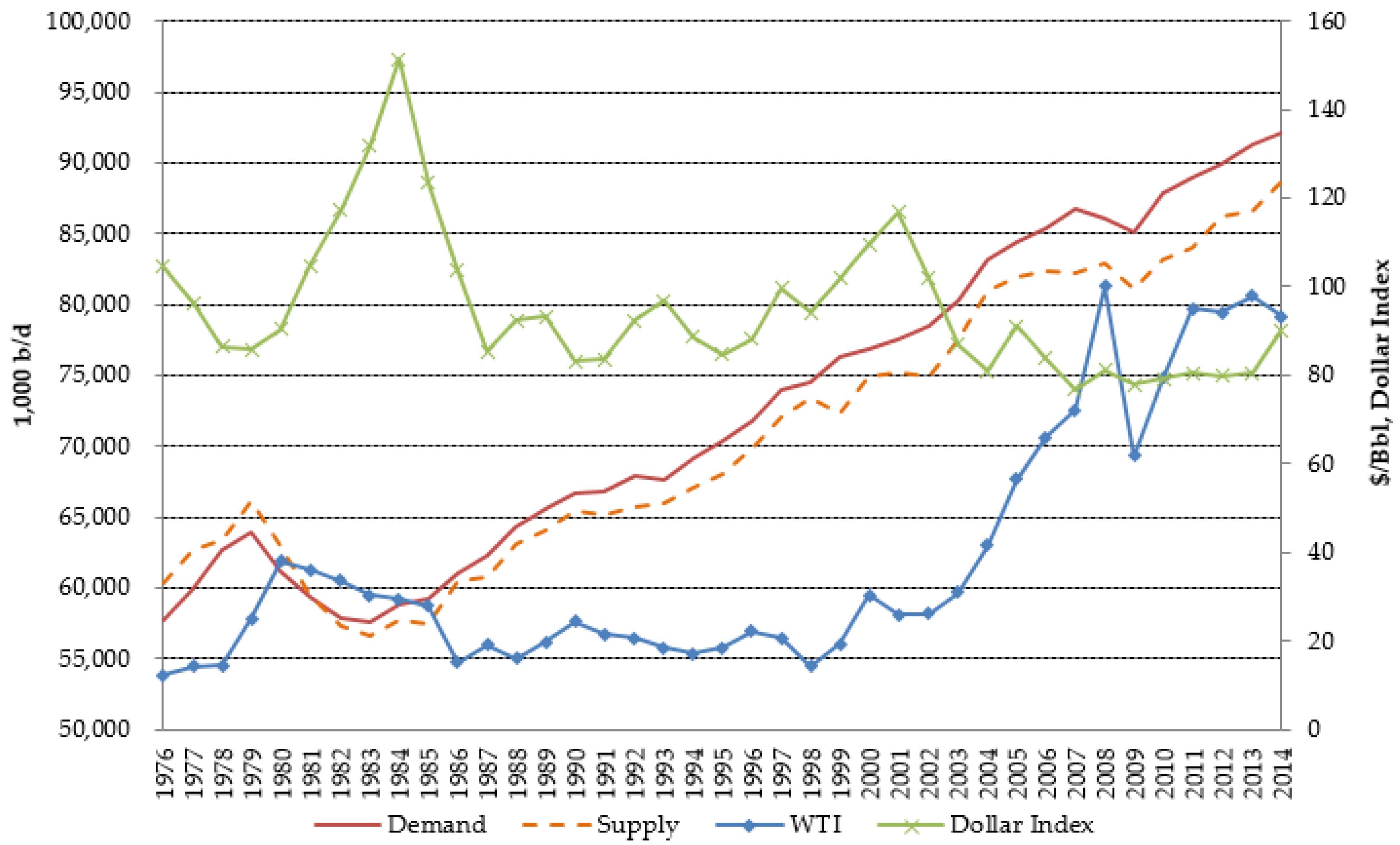
Table 2 summarizes the variables included in the forecasting model. The WTI spot price is used as the dependent variable, and world oil demand and supply, the US dollar exchange rate, upstream costs, and geopolitical event dummies are used as explanatory variables. The analysis examines 1976 to 2014 and the data trends during these periods are shown in
Figure 1.
3.2. Model Estimation
To estimate the proposed model, the parameters’ prior density function must first be set. As explained in
Section 3, a survey of expert judgment or researchers’ subjective opinions can be used for estimating the prior density function. Here, it was estimated using researchers’ opinions due to time limitations. Thus, any researchers using this model should be sufficiently informed to recognize the current status and future prospects of the oil market by monitoring market movements. To reflect the current status of the oil market (in which prices are significantly influenced by supply factors in response to the shale gas boom), this study uses prior information, weighting the factors as follows: 20% for world oil demand, 50% for world oil supply, 10% for the US dollar, 10% for upstream costs, and 10% for geopolitical events. The relative importance of variables is derived from estimates using the linear model and monthly data for the last three years of the estimation period, 2007–2009.
The Bayesian model is updated via the WinBugs program using available data on the past oil market. After updating the model, the constant terms are revised based on the final oil price in the time-series used in the estimation.
To test the goodness-of-fit and forecasting performance of the developed Bayesian models, OLS and neural network models are used as benchmarks. These models are widely used not only for forecasting oil prices but also for forecasting exchange rates and economic growth. By comparing the Bayesian models with these benchmarks, goodness-of-fit and forecasting performance can be assessed. The OLS model is estimated via Eviews. The neural network model carries out learning by placing explanatory variables in the input layer and dependent variables in the output layer. Through learning, the difference between the classification value generated and the actual value is gradually reduced to reach the final classification value. The input variables are transformed by a transfer function when transferred from the input layer to the middle layer or from the middle layer to the output layer. A Bipolar Sigmoid Function produced the best fit; it has the following configuration.
The model used here has four hidden layers for each variable (of six total, including a constant term). Therefore, 24 parameters were estimated (6 × 4).
The out-of-sample performance measure tests how accurately a model forecasts future demand using the given data. It evaluates the accuracy of the forecast demand by calculating the error between forecast estimates and actual demand data after dividing the period studied into estimating and forecasting periods. Mean absolute percentage error (MAPE) is used to measure the error between forecast demand estimates and actual demand data, as it is common in research on demand forecasting.
Here, is the estimated forecast, is the actual data, and is the observed period; MAPE measures the averaged forecasting error over period .
3.3. Testing Model Goodness-of-Fit
To test the goodness-of-fit of the proposed model, the oil price is estimated and compared to actual data; this is done using data on oil price determinants and WTI oil prices from 1976 to 2014. Since the results might differ according to the data used, comparative analysis was undertaken, running from the first 34 data-points to the final 38, in consecutive order.
Table 3 shows the goodness-of-fit of the proposed model and benchmark models. The best model at explaining past performance using past data is the neural network model. Most MAPE values for the neural network model are below 12%. This result stems from the flexibility of the neural network model: as it forecasts based on learning, not a normalized program, it explains the data best. A neural network model using a bipolar sigmoid function with a non-linear configuration has the highest estimation accuracy.
Indeed, the goodness-of-fit of both the proposed model and the OLS model is inferior to that of the neural network model. Since both models form a linear relationship between the explanatory and dependent variables, they are less flexible. The MAPE of the proposed model remains high after revising the constant terms because the revision was conducted using recent data; were it conducted over the whole period, the model goodness-of-fit would be better as the value of MAPE would be reduced. This is not done because the purpose of the proposed model is to maximize forecasting accuracy, not goodness-of-fit. If a model with excellent goodness-of-fit has inferior forecasting accuracy, it is likely worthless as a forecasting model. This is a central concern in forecasting studies. The goodness-of-fit is examined to understand the implications when comparing forecasting performance across models.
3.4. Testing the Models’ Forecasting Performance
To test the models’ forecasting performance, an out-of-performance test is conducted. This method compares a model’s forecast results with the recent actual data, with the model estimated using a dataset omitting this recent data.
Table 4 helps explain the concept of the out-of-performance test. Among these tests, one-step-ahead forecasts compare the model’s forecast for 2014 with the actual data for 2014, where the model is estimated after removing 2014 data from the set of available data, 1976 to 2014. Other forecasts, such as two-step-ahead or five-step-ahead forecasts, use analogous concepts.
The forecasting performance test, like the test of goodness-of-fit, uses the MAPE. As shown in
Table 5, the neural network model, which proved the best in terms of goodness-of-fit, shows poor results in the short term. However, its forecasting performance rapidly rises as the forecasting period becomes longer. The MAPE value for the neural network model in a three-step-ahead forecast is 2.29%, which is the best result. The neural network model also shows the second-best results in the four-step-ahead and five-step-ahead forecasts.
The proposed model has the best forecasting performance because it is estimated by subjectively reflecting the characteristics of the oil market in the prior parameter density function. This is a surprising result when considering the proposed model’s poor goodness-of-fit and highlights that even models with poor goodness-of-fit can have excellent forecasting performance. This result arises because the proposed model uses the structure of the oil market (which will change in the present or future) as the prior information for determining the parameters. The proposed model, which focuses on the structure of the oil market that will develop in the present or future, does not explain past oil prices well. However, the purpose of this study is to develop a model for forecasting future oil prices, not explaining the past, and the proposed model fits this purpose. Some principles recommend not to use the within-sample fit of the model to select the most accurate forecasting model [
70]. The OLS model shows a poor result in terms of goodness-of-fit but a strong result for short-term forecasting performance. This is because the constant of the estimated linear model is revised using time-series data for the final period. Such a linear model in which the constant term is revised seems simple but forecasts well.
As shown in
Table 5, five-step-ahead forecasting performance is poor for all models: all MAPE values exceed 5%. The models were estimated using data that changed rapidly from 2006 to 2013: oil prices rapidly increased from 2005 to 2008, drastically dropped in 2009, then again increased until 2011. The proposed model may solve such problems: if the signal that oil prices will suddenly rise is captured, the proposed model can accurately forecast oil prices by reflecting this information in the parameters’ prior density function. In the forecast results, only the 2014 characteristics were reflected in the parameters’ prior density function in order to fairly compare among models.
3.5. Forecasting the Long-Term Crude Oil Price
This section presents results of forecasting oil prices until 2040 using the proposed model. To estimate the model, the prior distribution of parameters from experts’ opinion is first set considering future trends in the oil market. We try to collect prior information based on reliable market reports including [
12,
13,
20,
35] and the authors’ insight into the oil market. The mean and variance of the normal distribution of parameters are set at the same value by the generic rule. This methodology is recommended to be used by researchers with expertise in the international oil market. Non-experts on the international oil market can gather prior information through survey of oil market experts.
OPEC’s market strategies have been attracting international concern in recent years, and their importance will grow in the future. As oil reserves of non-OPEC countries are drying up and major international oil suppliers’ ability to increase production is weakening, OPEC’s strategies will become more important factors. According to the long-term forecasts of the IEA and EIA, OPEC’s market share will increase from about 40% at present to over 60% after 2020, and over 90% of additional demand will depend on OPEC in 2040. Therefore, demand and supply in the global oil market will depend on OPEC’s market strategies (production policies); this study thus imposed a 40% weight on the prior distribution of the global supply variables.
Long-term oil prices will almost entirely depend on the global economic situation. If the global economy recovers in the future, global oil demand will increase. If there is a global economic recovery after 2016, global oil demand will steadily grow. Since oil demand factors are consistently important in determining the oil price, this study placed a weight of 30% on the prior distribution of the global demand variables. Since the possibility of a financial sector bubble (caused by the withdrawal of speculative funds and speculative demand) is expected to be low, this study imposed a 15% weight on the prior distribution of financial variables and a 7.5% weight on the prior distribution of variables related to upstream costs and geopolitical factors based on past trends, respectively. From the given relative importance of the variables, means of the prior distribution of the parameters are derived in Equation (8). The variances of the variables set at the same to means by the generic rule.
Table 6 depicts the estimated mean and standard deviation for the posterior distributions. According to the estimation results, more demand, less supply, lower dollar index, higher upstream cost, and geopolitical events positively affect the crude oil price.
4. Discussion and Conclusions
This study developed a model to forecast long-term oil prices that takes into account changes in the oil market and can inform government policies and business decision-making. A Bayesian approach, specifically a Bayesian normal multiple regression model with informative priors, was used for forecasting. World oil demand and supply, the financial situation, upstream costs, and geopolitical events were used in the model as factors affecting oil prices. To test the forecasting performance of the model, it was compared to estimates from OLS and neural network models. The goodness-of-fit was the best for the neural network model due to its flexibility, gained by connecting explanatory variables with dependent variables in a nonlinear form.
Because the goal was maximizing forecasting accuracy rather than goodness-of-fit, however, this study focused on the model with the best forecasting performance. On this test, the proposed model outperformed the linear and neural network models. The proposed model gained improved forecasting performance by reflecting recent and expected market information in its parameters using a prior density function. The linear model also showed good forecasting results by recalibrating its constant term based on recent market data. On the other hand, the neural network model lagged in forecasting performance. Because the oil market structure changes constantly, a neural network model, which reflects average past trends in parameters, has limits for predicting the oil market. However, the proposed model also has uncertainty because prior information on parameters depends on experts’ judgments. If experts misjudge the situation, they may forecast a distorted oil market. If experts understand the global oil market and have accurate intuition, however, the proposed model will have the best forecasting performance.
This study forecasts oil prices until 2040 using the proposed model and data on explanatory variables from the EIA. Greater relative importance was placed on oil supply based on a general consensus that the future oil market situation will depend on OPEC’s oil producing policies. The crude oil price was estimated to increase to $170/Bbl in 2040. The EIA and IEA have forecasted that in 2040 the oil price will reach $217/Bbl and $124/Bbl, respectively. The price estimated here is lower than the EIA estimate and higher than that of IEA because this study employs moderate assumptions regarding the future oil market—i.e., that the future market will not be tight and that a speculative bubble is unlikely.
This study is significant in two ways. First, it employed a Bayesian approach to develop a model that is able to explain the global oil market’s volatility and provide more accurate forecasts than those of previous studies. Second, while most oil price forecasting models have focused only on short-term forecasts, this study estimated long-term forecasts. Its results can thus contribute to preparing quick and accurate countermeasures to a rapidly changing oil market. For example, it is possible to predict transition speed to alternative energies including solar photovoltaic and wind. As public- and private-sector entities, such as airline companies and oil refineries, make long-term plans based on oil price forecasts, the price forecast here can be used to make policies and strategies in both of these sectors.
Several limitations of this study deserve mention. First, this study does not consider the possibility that oil price fluctuations may influence crude oil supply and demand. As the oil price rises, demand decreases and supply increases, and these changes then in turn influence the oil price again. This endogenous relationship has been captured in the recent strands of literature [
3,
6,
71,
72], although some earlier studies treated the price of oil as exogenous [
73,
74]. The Bayesian model suggested here cannot reflect this circular structure, while it focuses on improvements in forecasting accuracy. As another benchmark model, the vector autoregressive (VAR) model was used and estimated in this study, in order to reflect this endogenous relationship. Its estimation results are not presented on account of limited space. However, the results show lower forecasting accuracy. Models considering such endogenous relationships, such as the VAR model, have their own drawbacks for long-term forecasting; for example, see [
75,
76,
77] for further details. Therefore, an alternative model that relaxes the assumption of an exogenous relationship among the oil price, demand, and supply is required, which is a direction for future research. Second, the model presented in this study did not account for the possibility in variation of the relative importance over time. According to our preliminary analysis, relative importance varies over time. We analyzed the variation of relative importance from 1996 to 2009 and obtained relevant results. The variation of relative importance over time has its roots in different reasons. For example, a structural shift in oil market power is highlighted by previous studies [
78,
79]. However, the central part of our study is to enhance forecasting accuracy by using both experts’ judgment and available market data. Our model partly overcomes the assumption of constant relative importance by updating itself with available market data. Moreover, as the oil market dynamics are changing continuously, it may not be very meaningful to assume future variation in relative importance at the present point of time. In order to address time variation in the relative importance, however, the presented model can produce an updated forecasting result periodically with a different relative importance. A Bayesian model with time-varying coefficients may also be a possible alternative.


