Article

Characteristics of Particulate Pollution (PM2.5 and PM10) and Their Spacescale-Dependent Relationships with Meteorological Elements in China

1
College of Environmental Science and Engineering, Hunan University, Changsha 410082, China
2
Key Laboratory of Environmental Biology and Pollution Control (Hunan University), Ministry of Education, Changsha 410082, China
3
School of Public Health, University of California, Berkeley, CA 94720, USA
4
College of Mathematics and Econometrics, Hunan University, Changsha 410082, China
*
Author to whom correspondence should be addressed.
Sustainability 2017, 9(12), 2330; https://doi.org/10.3390/su9122330
Submission received: 14 November 2017 / Revised: 4 December 2017 / Accepted: 5 December 2017 / Published: 14 December 2017

Abstract

:
Particulate matter (PM) pollution in China has an obvious characteristic of spatial distribution. It is well known that intensive anthropogenic activities, such as fossil fuel combustion and biomass burning, have great influence on the spatial distribution of PM pollution. However, the spacescale-dependent relationships between PM concentrations and weather conditions remain unclear. Here, we investigated the characteristics of two types of particulate pollution, including PM2.5 and PM10, and their spatial relationships with meteorological elements in 173 cities throughout China from March 2014 to February 2015. Results: (1) High PM2.5 concentrations were distinctly located southeast of the Hu Line, and high PM10 concentrations were distinctly situated north of the Yangtze River; (2) Spacescale-dependent relationships were found between PM pollution and meteorological elements. The influence of temperature had similar inverted V-shaped characteristics, namely, there was serious PM pollution when temperature was about 15 °C, and there was slight PM pollution when temperature was less or more than 15 °C. Annual precipitation, wind speed, and relative humidity were negatively correlated with PM, while annual atmospheric pressure was positively correlated with PM; (3) The ideal meteorological regions were identified according to the quantified spatial relationships between PM and meteorological elements, which could be defined by a combination of the following conditions: (a) temperature <10 °C or >21 °C; (b) precipitation >1500 mm; (c) atmospheric pressure <900 hPa; (d) wind speed >3 m/s; and (e) relative humidity >65%, where air pollutants can easily be scavenged. The success of this research provides a meteorological explanation to the spatial distribution characteristics of PM pollution in China.

Graphical Abstract

1. Introduction

Air pollution is a global epidemic, caused by chemical and biological molecules, and particulate matter (PM), which results in various environmental and human health impacts. Many studies have shown that ambient air pollution is related to public health, ecological plant growth, and regional and global climates [1,2,3,4,5,6,7]. A critical component of air pollution is atmospheric PM, which includes fine particles with small diameters that remain suspended in air and do not settle. PM10 denotes particles with an aerodynamic diameter of 10 µm or less, and PM2.5 denotes those with a diameter of 2.5 µm or less. High concentrations of air particulates can have environmental impacts, such as degraded atmospheric visibility, and human impacts, such as acute or chronic respiratory diseases [8,9,10,11,12,13,14,15]. Between 1990 and 2005, global population-weighted PM2.5 increased by 6%, with noted increases in Asia [16]. In recent years, some mega-cities in China, particularly during winter in the northern regions, have experienced serious and continuous haze pollution [17], which has resulted in an increased interest in exploring the chemical characteristics and the source apportionment of PM [18,19]. The dire situation has led some environmental staffers in polluted regions, such as Beijing, to attempt to mitigate air pollution by adopting a series of control measures, including adjusting industrial structure, using clean energy, limiting the number of private cars, and establishing the joint prevention and control work with neighboring provinces [20,21].
In the spatial scale, high aerosol PM concentrations are a regional phenomenon [22], with a distinct characteristic of spatial agglomeration. The North China Plain is the predominant region of agglomeration [23]. In the temporal scale, the annual and seasonal variation characteristics of PM have been observed in many cities and regions [23,24,25]. In the spatial distribution of PM2.5, the Hu Line [26] and the Yangtze River are the E–W divide and S–N divide between high and low values of China, respectively. Wang, et al. [27] explored the drivers of PM2.5 distribution in China from the perspectives of human activities, such as urban area, urban population, and industrial production.
At present, considerable research has been carried out on the relationships between PM and meteorological factors. For example, Li, Qian, Ou, Zhou, Guo, and Guo [24], Zhang et al. [28] and Tian, Qiao, and Xu [25] have analyzed the impacts of meteorological conditions on PM pollution in different season. Jian et al. [29], Li et al. [30], and Qin et al. [31] have predicted PM concentrations using meteorological data. However, most studies have some limitations, due to their analyses focusing on a certain city or region, which is hard to reflect back to the whole state of PM pollution [24,25,28]. Moreover, fewer research studies have analyzed the impact of meteorological factors on the spatial distribution of PM, particularly in the large spatial scale, such as the whole country.
It is well known that there are various climatic zones and meteorological conditions with obvious differences between regions across China. In other words, meteorological conditions also have regional phenomenon in a spatial distribution, just like the spatial agglomeration of high PM2.5 concentrations [23]. This informs us that the spatial distribution characteristics of PM pollution may be caused by the spatial difference of meteorological conditions. Hence, this study is designed to quantify the spatial relationships between PM pollution and meteorological elements in China for the first time.
In the study, five meteorological elements, including precipitation, relative humidity, temperature, pressure, and wind speed, were investigated. Here, we first describe the spatial distribution of PM (including PM2.5 and PM10) and meteorological elements, and compare their spatial characteristics by calculating the similar degree of association between PM and meteorological elements. And then, we provide a quantitative analysis to understand meteorological drivers of PM pollution. The purpose of this study is to find out the ideal meteorological regions where high PM concentrations are easily scavenged. The work is particularly useful for urban industrial layout, because adverse meteorological regions can facilitate the air pollution if the polluting enterprises are assigned to regions.

2. Materials and Methods
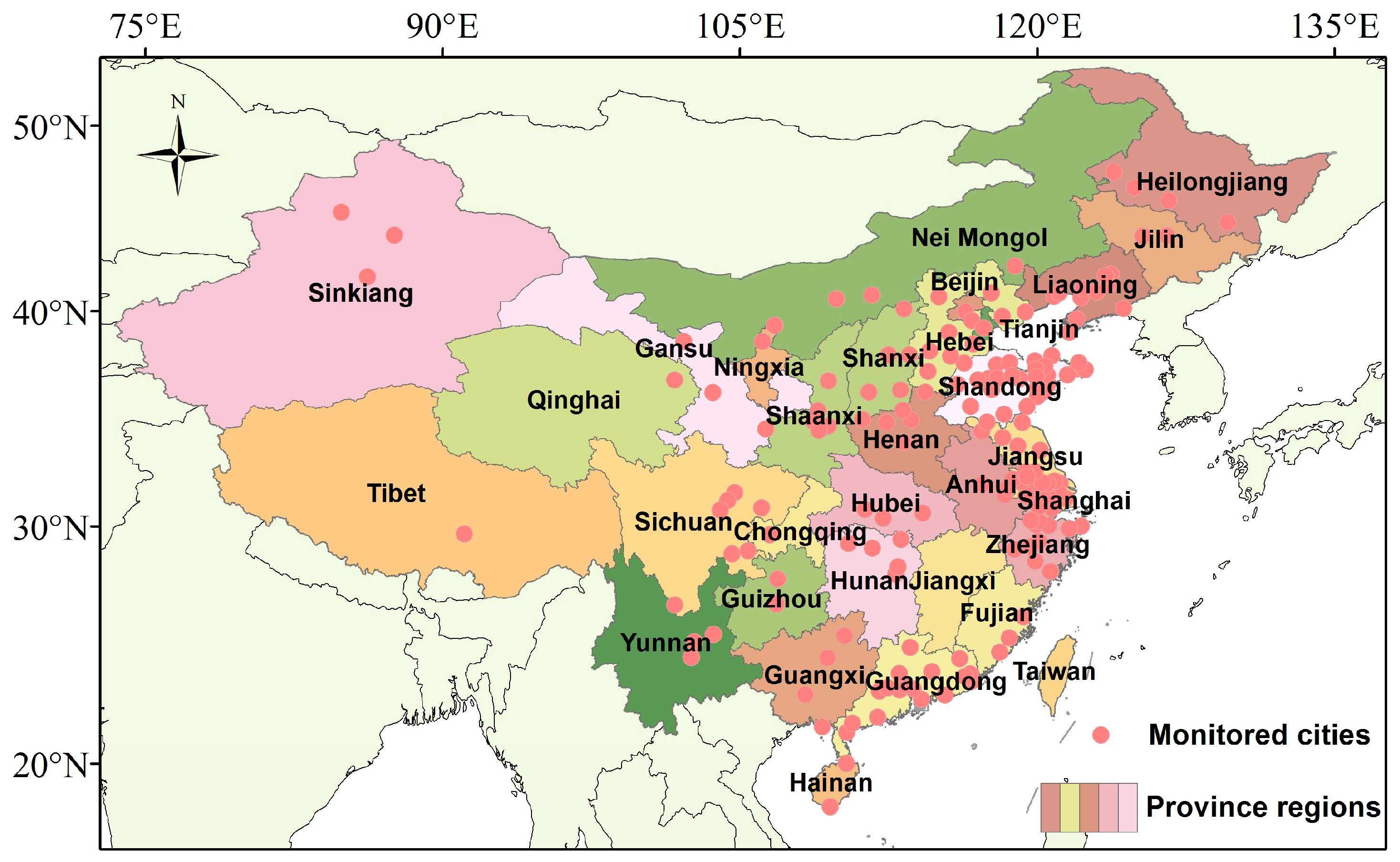
2.1. Data Source

For the one-year period from March 2014 to February 2015, the datasets of atmospheric PM and meteorological elements (including precipitation, relative humidity, temperature, pressure, and wind speed) were collected from 173 Chinese cities, as shown in Figure 1. Daily records of particulate concentrations (PM2.5 and PM10) were obtained from the Chinese Air Quality On-line Monitoring Analysis Platform (www.aqistudy.cn/historydata). Meteorological data, including precipitation, relative humidity, temperature, pressure, and wind speed were obtained from Weather Underground (www.wunderground.com). The annual average values were calculated to explore the spatial relationships between particulates and meteorological factors for the 173 cities. Hence, in the study, all data types were analyzed in the form of annual average values.

2.2. Spatial Interpolation for PM and Meteorological Elements

Spatial interpolation methods for PM (including PM2.5 and PM10) and meteorological elements allow for an accurate assessment and monitoring of spatial distribution information. In recent years, many scholars have studied spatial interpolation methods [32,33]. The most widely used methods include the inverse distance weighted method, the moving average method, the Kriging method, and the spline function method. Of these, the Kriging method is most suitable for meteorological interpolation because expert knowledge and physical processes are not needed, which can effectively reduce anthropogenic influence and improve the accuracy of the interpolation [34]. In this study, the Kriging method was used to interpolate the annual average values of particulate concentrations and meteorological factors from historical data.
According to the statistical hypothesis, sample size and uniformity of sample distribution are decisive for the result of interpolation. In this study, 173 major cities throughout China were selected as the interpolation sample. The annual average values of PM concentrations and various meteorological elements were calculated, and spatially interpolated in GIS to obtain spatial distribution maps.

2.3. The Role of Meteorological Elements in Relation to PM

As mentioned in some previous studies [24,35], there are obvious nonlinear relationships among meteorological elements. Therefore, a reasonable and effective reasonable assessment of these relationships is of great importance. Traditional statistical methods, such as the Spearman’s rank correlation and the gray correlation analysis can result in poor assessment quality, and may cause a large error [25,28,31,36]. To overcome these hurdles, new methodologies have been developed for classification and regression, such as neural network and boosted regression tree (BRT), which offer advantages over interaction and prediction [37,38]. Tree-based methods can deal with a mix of variables effectively, including continuous, categorical, and even missing data. Additionally, trees can successfully model nonlinear effects and interactions between meteorological elements [38]. So, in the study, we used the boosted regression tree (BRT) model to quantify the effects of meteorological elements on China’s PM (including PM2.5 and PM10) concentrations. A summary of these meteorological elements can be found in Figure 2.
The BRT model can be used to predict and explain potential relationships between a response and its predictor variables. The BRT model can effectively handle many types of numerical or categorical responses and predictors and loss functions such as Gaussian, Laplace, Bernoulli, and Poisson [39]. In the current study, the Gaussian distribution was used to explore the impacts of meteorological factors on PM2.5 and PM10. The BRT model was substantially different from traditional regression-based approaches, which were designed to improve the performance of a single model by fitting and combining many models for prediction. The BRT model contains two robust algorithms: regression trees and boosting. The regression trees technique eliminates interactions among predictors by recursive binary splits, while the boosting algorithm uses an iterative method to develop a tree ensemble consisting of many small regression trees to improve stability and predictive performance [37,40].
Previous studies have explored the use of BRT models to draw inferences concerning various intricate predictor variables. Carslaw and Taylor [41] analyzed the influence of each variable on nitrogen oxide (NOx) concentrations at a mixed source location using the BRT method. Similar research was conducted by Sayegh, Tate, and Ropkins [40] regarding roadside NOx concentrations, which also considered multiple variables, including background concentrations of NOx, traffic density, and meteorological conditions. In recent years, BRT models have been used for epidemiological studies, such as hand, foot and mouth disease [42,43,44].
In the BRT model, the three model input parameters are the learning rate (lr), tree complexity (tc), and number of trees (nt). These values need to be determined for model fitting purposes. The learning rate is a shrinkage parameter for reducing the contribution of each tree as it is added to the model during the expansion process. The tree complexity determines the maximum depth of variable interactions that control the size of the trees. In general, decreasing lr increases the number of trees required, and tc influences the optimal nt. For a given lr, fitting more complex trees results in fewer trees required for minimum error. To achieve the best predictive performance and minimum predictive error, it is necessary to determine the optimum combination of the three parameters (lr, tc, and nt). As expected, predictive performance is also affected significantly by sample size, and large samples produce lower predictive error. However, in most situations, large amounts of sample data are not available, so techniques such as cross validation (cv) are employed to develop and evaluate the model. In this study, the three model parameters (lr, tc, and nt) were determined using 10-fold cross validation (cv) [45]. To obtain the optimal values of these parameters, many simulations were carried out using the following values: lr (0.5–0.001), tc (1–10), and nt (100–15,000). As recommended [37], lr = 0.005 and tc = 5 were used, and nt > 1000 was optimal.
All simulations were performed with R statistics software using the “gbm” package version 2.1.3 developed by Greg Ridgeway [39]. The whole dataset was divided into two parts: one used as the training dataset to develop the model, and the other used as the independent testing set to estimate the prediction performance. With a bag fraction of 0.5, half of the training set was randomly selected to fit each consequent tree.
In the BRT model, PM concentrations were the response variables, and five meteorological elements were the predictor variables. Correlation coefficients between the response and predictors were calculated to display the similar degree of association between PM and meteorological elements. The contribution of each predictor was calculated to weigh its relative importance in atmospheric PM. Partial dependence plots were produced to show the influence of each meteorological variable on the PM concentrations, with variation in the meteorological variable.

3. Results and Discussion

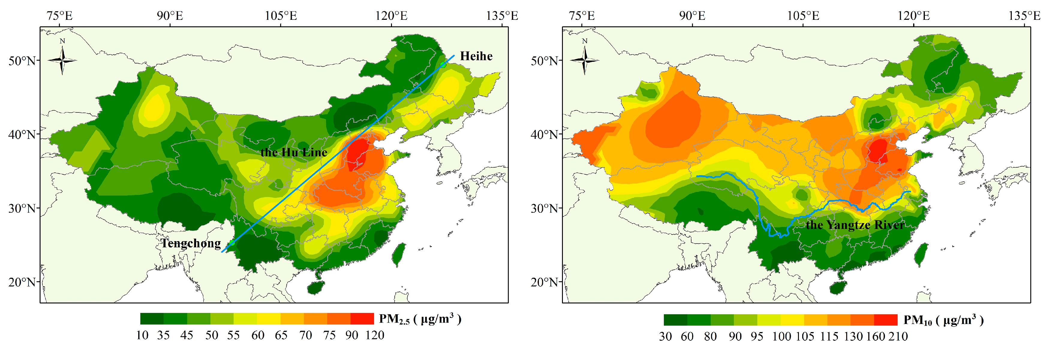
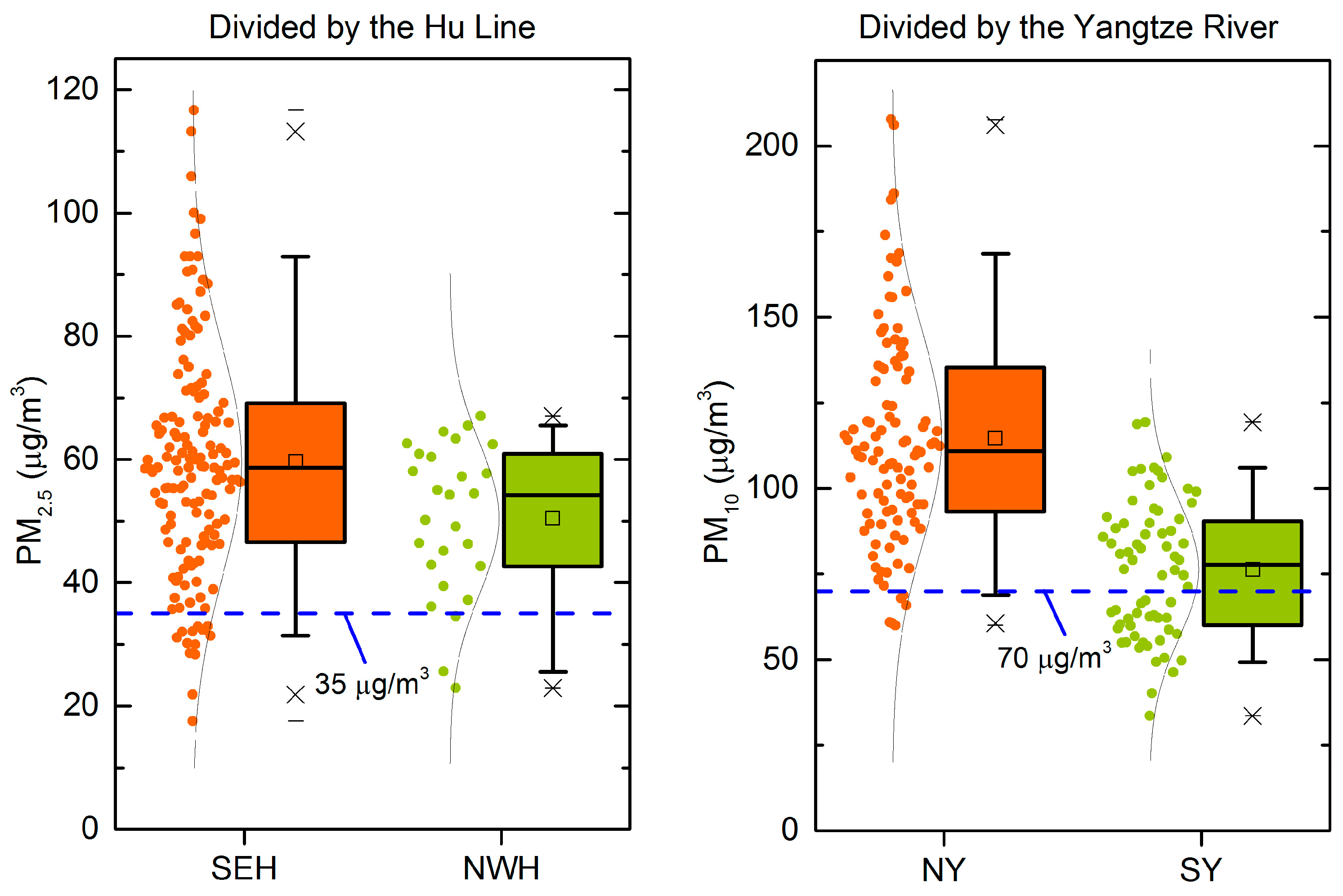
3.1. Spatial Distribution Characteristics of PM

Figure 3 enables the visualization of PM (including PM2.5 and PM10) spatial distributions as calculated through Kriging interpolation based on 173 monitoring cities, during the year of 2014. Results indicated that there were remarkable distribution differences between PM2.5 and PM10. PM2.5 concentrations were shown to be generally higher in cities situated southeast of the Hu Line (SEH) than those situated northwest of the Hu Line (NWH). However, PM10 concentrations were observed to be significantly higher in cities located north of the Yangtze River (NY) than those located south of the Yangtze River (SY). Figure 4 details the differences of PM2.5 and PM10, divided respectively by the Hu Line and the Yangtze River. The annual mean PM2.5 level ranged from 59 ± 19 μg/m3 in cities situated SEH, to 50 ± 12 μg/m3 in cities situated NWH. They far exceeded the Chinese pollution standard of 35 μg/m3 for “good health” [46]. We found only 13 (or 8.9%) of the 146 monitored cited situated SEH and 3 (or 1.1%) of the 27 monitored cited situated SHE to have confirmed with the annual standard. Meanwhile, the annual mean PM10 level ranged from 115 ± 31 μg/m3 in cities located NY, to 76 ± 20 μg/m3 in cities located SY. Among them, PM10 in cities located NY far exceeded the Chinese pollution standard of 70 μg/m3 for “good health” [46], while PM10 in cities located SY was close to the annual standard. We found only 6 (or 5.7%) of the 105 monitored cited located NY to have conformed with the annual standard. But for the 68 monitored cited located SY, there were 29 (or 42.6%) cities meeting the annual standard. Further, the ratio of PM2.5 to PM10 in China was calculated, as exhibited in Figure 5. Results indicated that there was a wide distribution range of 30–70% for the ratio of PM2.5 in PM10. In the regions situated SEH, the ratio of PM2.5 to PM10 exceeded 50%, which indicated PM2.5 was the major component in PM10 during the regions. However, in the regions located NWH, the ratio of PM2.5 to PM10 was less than 50%. Particularly in partial regions of Sinkiang and Inner Mongolia, the ratio was under 40%.
We pose two main reasons for this pattern. Firstly, the variance is due to different pollutant sources. Fossil fuel combustion and biomass burning are likely to increase the concentrations of PM2.5, particularly in densely populated areas such as those southeast of Hu Line [47]. PM10, different from PM2.5, mostly originates from the dust blown by the wind, especially from the surfaces without cement and asphalt. In the areas located NY, the soil is drier and contains less water; as a result, dust is more easily blown into the air, and can cause sandstorms and increase PM10 [48,49,50]. Then, because the size distribution of PM10 is more extensive than that of PM2.5, the regions polluted by PM2.5 also suffer from PM10 pollution. Therefore, the regions polluted by PM2.5 and PM10 are either the same or different in the spatial distribution. Particularly, in the regions situated SEH, PM2.5 is the main PM contributor (above 50%). Due to the mechanism of impact on human health, PM2.5 is more harmful than PM10, so at the same PM levels, a higher ratio of PM2.5 to PM10 indicates a more adverse impact on human health. Secondly, we highlight the impact of climatic conditions on the spatial distribution of PM. Though human activities are the main contributors to PM pollution and Wang, Zhou, Wang, Feng, and Hubacek [27] have explored the role of socioeconomic factors in relation to PM2.5 concentrations in the spatial scale in China, climatic elements cannot be ignored. For example, there is higher precipitation and relative humidity in regions situated SY than those located in the northern regions, which is vital to eliminate pollutants in the air. In addition, the wind speed on the southeast of coast of China is higher than that on the central China, which contributes to the pollution dispersion [24].

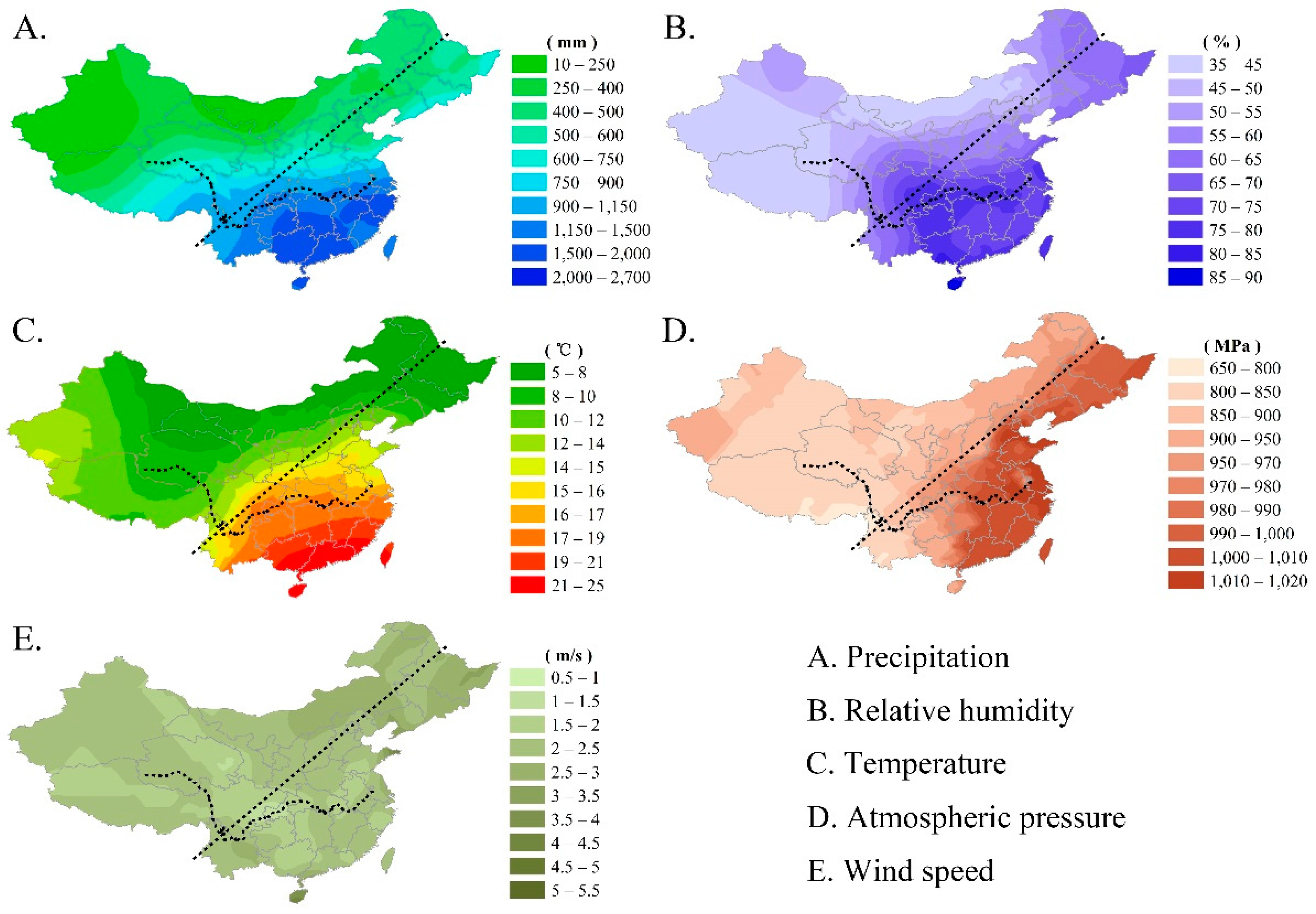
3.2. Similar Spatial Characteristics between PM and Meteorological Elements

It is interesting to investigate the potential drivers of PM in spatial distribution in China. It is also well known that there are various climatic zones and weather conditions which have obvious differences between regions in China. This informs us that the spatial distribution characteristics of PM may be partly caused by the spatial difference of meteorological conditions.
In the study, we found that temperature, relative humidity, wind speed, atmospheric pressure and precipitation presented a consistently significantly coherence with particulates (PM2.5 or PM10) in the spatial distribution through the annual average data. The spatial distribution characteristics of investigated meteorological factors can be clearly seen from Figure 6A–E. The spatial variations in precipitation and temperature were similar to that in PM10, and high precipitation and high temperatures appear south of the Yangtze River (SY). The spatial variations in atmospheric pressure were similar to that in PM2.5, and the region situated southeast of the Hu Line (SEH) had high pressure. The spatial variations in relative humidity were similar to those in both PM2.5 and PM10. The spatial variations in wind speed were similar to that in PM2.5, and high wind speed was located in northwest of the Hu Line (NWH) and south of the Yangtze River (SY).
In consideration of the nonlinear relationships among meteorological factors, further analysis was carried out through the boosted regression tree method. The correlation coefficients of verification and cross validation exhibited high similar degrees of association between particulates and meteorological factors (Figure 7), reaching to 0.938 (between PM2.5 and meteorological factors) and 0.917 (between PM10 and meteorological factors), respectively. Among these meteorological factors, temperature was the main contributor and had the largest contributions to both of PM2.5 and PM10, which were respectively 29.8% and 39.4%. This may be due to different temperature requires different energy demands for heating (or cooling). In addition, precipitation and atmospheric pressure played a significant role in the spatial distribution of PM2.5, accounting for 22.8% and 19.4%. In terms of the spatial distribution of PM10, relative humidity (35.1%) and precipitation (17.1%) had a great influence, to some extent.
In fact, in the spatial distribution, Hu Line is an important boundary line in the distribution of the Chinese population within mainland China [26]. According to a seminal theory [51], the formation of the Hu Line is the product of climate change. In the evolution of nearly a thousand years, climate change has resulted in fluctuation in the agricultural production potential in China; the population followed this change and formed the geographical boundary line of population distribution. Further, in the densely populated areas, large amounts of fossil fuel and biomass are consumed, and particulate pollution is generated. Thus, in spatial distribution characteristics of PM, meteorological elements are the direct or indirect contributors in China.

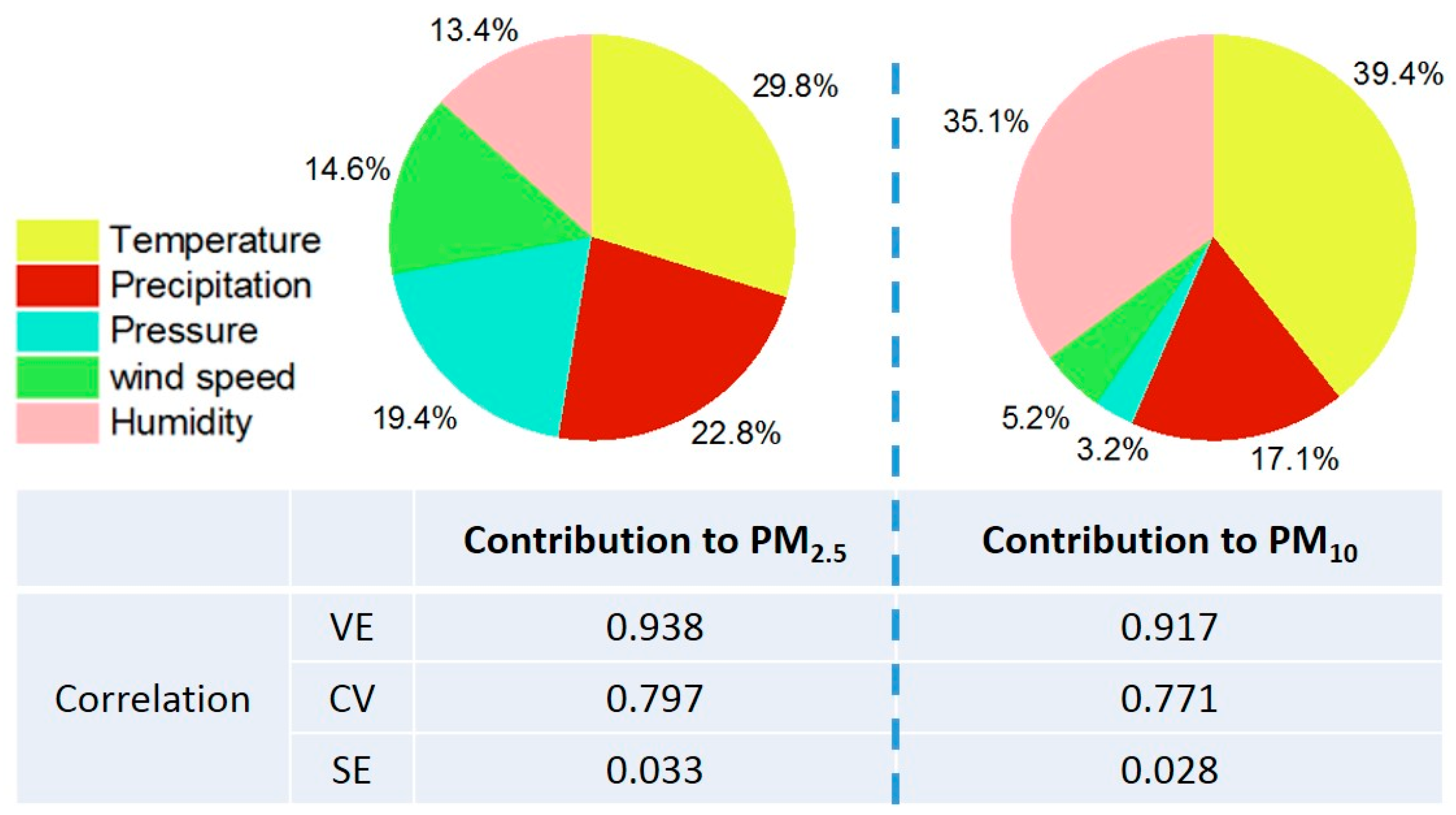
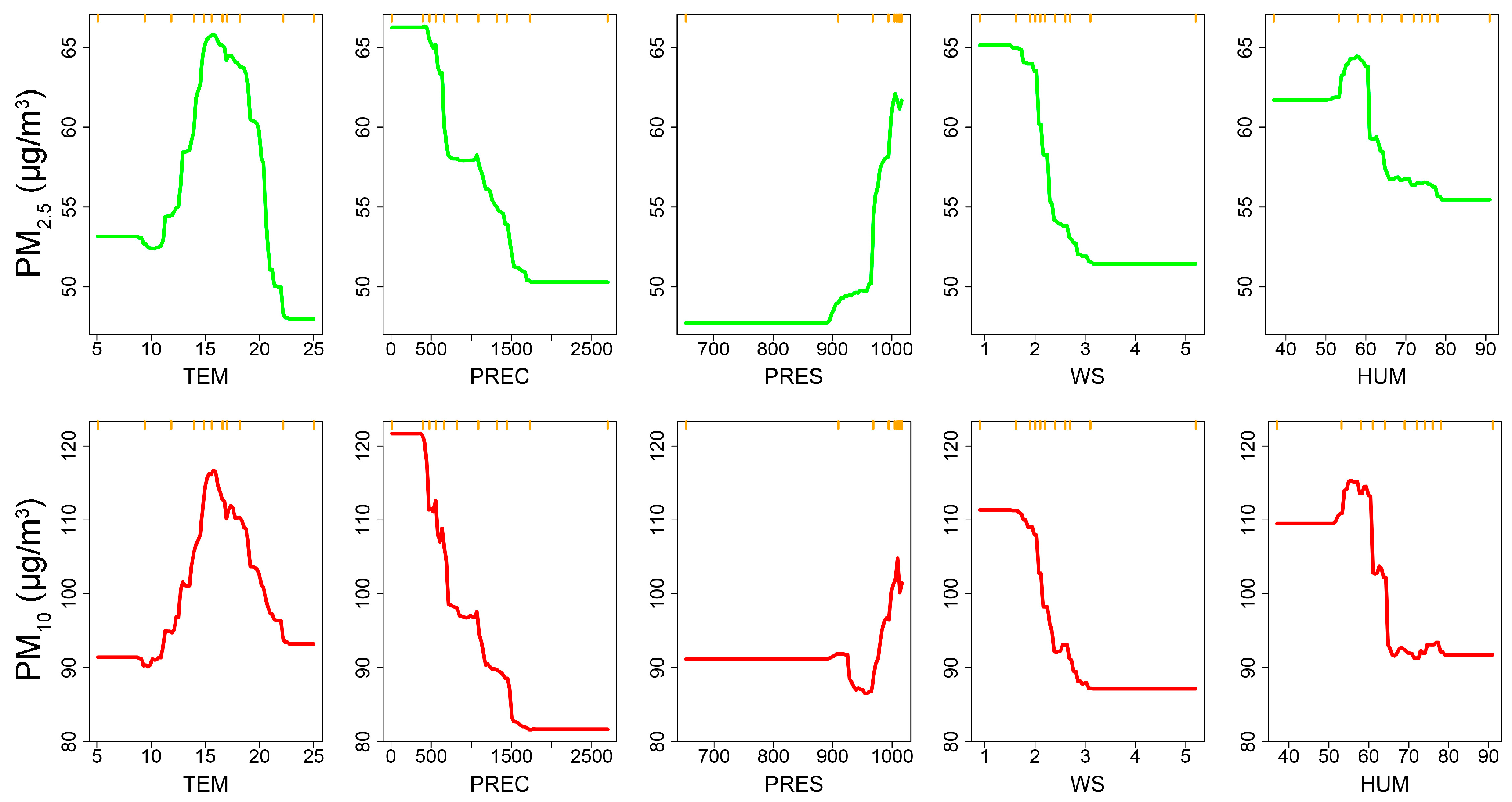
3.3. Correlation between Air PM and Meteorological Elements

The boosted regression tree model was used to quantify the spatial relationships between PM (including PM2.5 and PM10) and meteorological elements across China, as shown in Figure 8. It could be clearly observed that the relationship curves of PM2.5-meteorological factors were very similar to those of PM10-meteorological factors. The results indicated that the influence of meteorological factors on the spatial distribution of PM2.5 was the same as that of PM10. For this reason, PM2.5 and PM10 were subsequently considered the same, and denoted simply as PM.
There existed three threshold points on the PM–temperature curve. When the temperature was above 10 °C, PM concentrations were increasing until the second threshold point (approximately 15 °C), after which PM concentrations began to decrease. When the temperature approached 21 °C, the trend of the curve began to be flattened. In other words, the regions where temperature was 15 °C, such as Beijing–Tianjin–Hebei regions, had the highest PM concentrations. On the contrary, in the southeastern regions in China, where the temperature was above 15 °C, there was low PM concentrations. This is due to the fact that high temperature normally accompanies a higher boundary layer, and promotes the vertical dispersion of particles within the atmosphere [24].
The finding that precipitation was negatively correlated with PM concentrations until a threshold point (1500 mm), is in accordance with the fact that the air quality is better in rainy areas. The negative correlation indicates high precipitation can decrease the PM concentrations, due to its scavenging effects on polluted air.
In this study, the PM–atmospheric pressure curve did not increase until 900 hPa. When the atmospheric pressure was above 900 hPa, the trend of the curves began to rise. Generally, when an area has low atmospheric pressure, air converges and rises. Particulates in the near surface rise to higher altitudes, accelerating the dispersion and dilution of air pollutants. Conversely, when an area is controlled by a high atmospheric pressure, the air becomes stable in the vertical direction, which hinders pollutant dispersion [24]. What’s more, the contribution of atmospheric pressure to PM2.5 (19.4%) was larger than the contribution to PM10 (3.2%), as shown in Figure 7. Compared to coarse particulate (PM10), fine particulate (PM2.5), due to its lower gravity, may be more sensitive to the influence of atmospheric pressure, and can be transported by ascending gas flow. For the coarse particulate (PM10), however, it is opposite, due to its more gravity than PM2.5. Hence, the regions located northwest of the Hu Line (NWH), under the impact of low atmospheric pressure, are more polluted by PM10, not by PM2.5.
As with the relationship between PM and precipitation, PM and wind speed are negatively correlated until a threshold point around 3 m/s, which means high wind speed contributes to the dispersion of air PM. The regions situated NWH are controlled by high wind speed, so the air quality is better. For the cross region situated SEH and NY, particularly in the Beijing–Tian–Hebei region, though the wind speed is high, the PM pollution remains serious, which is mainly caused by the contribution of regional transport under the impact of high wind speed [52,53]. It could be clearly observed that the regions located NWH were polluted by PM10, not by PM2.5 (Figure 3). This is because PM10 mostly originates from the dust blown by the wind, especially from the surfaces without cement and asphalt. In the regions located NWH, the soil is drier and contains less water; as a result, dust is more easily blown into the air, and can cause sandstorms and result in high PM10 concentrations [48,49,50].
The PM–relative humidity curve had the trend of increasing when the relative humidity ranged 50–60%, and then decreased rapidly until a threshold point around 65%. Generally, the air quality was worse in the low relative humidity, and better in the high relative humidity. In the regions under the impact of high relative humidity, the air particulates absorb more water, increase in size and volume, and subside to the ground with the gravity [54]. Moreover, high relative humidity may also indicate more precipitation events, which results in lower PM concentrations [55]. In the spatial distribution, the southern regions in China had little particulate pollution, due to higher relative humidity, which is in accordance with the theory. In the Beijing–Tianjin–Hebei regions, because of the higher pollutant emission and lower relative humidity, the air quality is obviously worse than other regions. However, the regions northwest of Hu Line are not polluted by PM2.5, though the regions are controlled by the low relative humidity. This is mainly due to PM2.5 originating from fossil fuel combustion and biomass burning [56], but these regions have little pollutant emission because of the sparse population.
The study reveals that there are spacescale-dependent relationships between PM pollution and meteorological elements. The spacescale-dependent relationship informs us that the meteorological conditions influence PM concentrations in the spatial distribution. In summary, the regions with temperature (less than 10 °C or more than 21 °C), precipitation (above 1500 mm), atmospheric pressure (below 900 hPa), wind speed (above 3 m/s), and relative humidity (above 65%), have great air quality. In view of the constraints of reality, we selected the top three influential factors, namely, temperature (29.8–39.4%), relative humidity (13.4–35.1%), and precipitation (17.1–22.8%) as the filter conditions to evaluate the air quality in a certain area. Results indicate that the regions on the southeast coast of China may be the most appropriate for urban industrial production. Meanwhile, the air pollutants emitted by industrial production are easy to be scavenged.

4. Conclusions

This study showed the spatial characteristics of PM pollution and related meteorological elements. Using the boosted regression trees analysis, we quantified the spatial relationships between PM concentration and meteorological elements. Results indicated that climatic factors were important driving forces influencing the spatial agglomeration of PM concentrations, besides anthropogenic activities. The influence of temperature had similar inverted V-shaped characteristics, and the regions with annual temperature around 15 °C were most polluted by PM. The annual PM concentrations were negatively correlated with annual precipitation, wind speed, and relative humidity, but they were positively correlated with annual atmospheric pressure. According to our analysis, the ideal meteorological regions were defined by a combination of the following conditions: (a) temperature <10 °C or >21 °C; (b) precipitation >1500 mm; (c) atmospheric pressure <900 hPa; (d) wind speed >3 m/s; and (e) relative humidity >65%, where air pollutants are easily scavenged. Our study provides another explanation to the regional agglomeration phenomenon of PM pollution that climatic distribution greatly influences spatial characteristics of PM concentrations, just like anthropogenic activities.
However, there are some limitations to the present research. First, the study period was based on a one-year dataset from March 2014 to February 2015, which may be short for the exploration to the spatial relationships between PM pollution and weather conditions. Second, the PM pollution dataset was collected from urban regions, not including rural regions. The spatial characteristics of PM pollution could be overestimated. Third, the meteorological elements only include precipitation, relative humidity, temperature, atmospheric pressure, and wind speed. Maybe wind direction and cloud cover also have influence on the spatial distribution of PM, which can be considered together in further research.

Acknowledgments

This work was sponsored by National Nature Science Foundation of China (51579094, 51679082, 51521006 and 51479072).

Author Contributions

Xiaodong Li and Xuwu Chen conceived, designed and performed the research; Xuwu Chen wrote the paper; Xingzhong Yuan, Guangming Zeng, Tomás León, Jie Liang, Gaojie Chen and Xinliang Yuan analysed the data.

Conflicts of Interest

The authors declare no conflict of interest.

References

  1. Garcia-Menendez, F.; Saari, R.K.; Monier, E.; Selin, N.E. U.S. Air Quality and Health Benefits from Avoided Climate Change under Greenhouse Gas Mitigation. Environ. Sci. Technol. 2015, 49, 7580–7588. [Google Scholar] [CrossRef] [PubMed]
  2. Hirabayashi, S.; Nowak, D.J. Comprehensive national database of tree effects on air quality and human health in the United States. Environ. Pollut. 2016, 215, 48–57. [Google Scholar] [CrossRef] [PubMed]
  3. Sicard, P.; Augustaitis, A.; Belyazid, S.; Calfapietra, C.; de Marco, A.; Fenn, M.; Bytnerowicz, A.; Grulke, N.; He, S.; Matyssek, R.; et al. Global topics and novel approaches in the study of air pollution, climate change and forest ecosystems. Environ. Pollut. 2016, 213, 977–987. [Google Scholar] [CrossRef] [PubMed]
  4. Tambo, E.; Duo-Quan, W.; Zhou, X.N. Tackling air pollution and extreme climate changes in China: Implementing the Paris climate change agreement. Environ. Int. 2016, 95, 152–156. [Google Scholar] [CrossRef] [PubMed]
  5. Wu, Y.; Zhang, F.; Shi, Y.; Pilot, E.; Lin, L.; Fu, Y.; Krafft, T.; Wang, W. Spatiotemporal characteristics and health effects of air pollutants in Shenzhen. Atmos. Pollut. Res. 2016, 7, 58–65. [Google Scholar] [CrossRef]
  6. Zheng, J.; Jiang, P.; Qiao, W.; Zhu, Y.; Kennedy, E. Analysis of air pollution reduction and climate change mitigation in the industry sector of Yangtze River Delta in China. J. Clean. Prod. 2016, 114, 314–322. [Google Scholar] [CrossRef]
  7. Liang, J.; Feng, C.; Zeng, G.; Zhong, M.; Gao, X.; Li, X.; He, X.; Li, X.; Fang, Y.; Mo, D. Atmospheric deposition of mercury and cadmium impacts on topsoil in a typical coal mine city, Lianyuan, China. Chemosphere 2017, 189, 198–205. [Google Scholar] [CrossRef] [PubMed]
  8. Brauer, M.; Freedman, G.; Frostad, J.; van Donkelaar, A.; Martin, R.V.; Dentener, F.; van Dingenen, R.; Estep, K.; Amini, H.; Apte, J.S.; et al. Ambient Air Pollution Exposure Estimation for the Global Burden of Disease 2013. Environ. Sci. Technol. 2016, 50, 79–88. [Google Scholar] [CrossRef] [PubMed]
  9. Idris, I.B.; Ghazi, H.F.; Zhie, K.H.; Khairuman, K.A.; Yahya, S.K.; Abd Zaim, F.A.; Nam, C.W.; Abdul Rasid, H.Z.; Isa, Z.M. Environmental Air Pollutants as Risk Factors for Asthma Among Children Seen in Pediatric Clinics in UKMMC, Kuala Lumpur. Ann. Glob. Health 2016, 82, 202–208. [Google Scholar] [CrossRef] [PubMed]
  10. Jie, L.; Peng, Y.; Wensheng, L.; Agudamu, L. Comprehensive Assessment Grade of Air Pollutants based on Human Health Risk and ANN Method. Procedia Eng. 2014, 84, 715–720. [Google Scholar] [CrossRef]
  11. Xu, S.; Zhang, W.; Li, Q.; Zhao, B.; Wang, S.; Long, R. Decomposition Analysis of the Factors that Influence Energy Related Air Pollutant Emission Changes in China Using the SDA Method. Sustainability 2017, 9, 1742. [Google Scholar] [CrossRef]
  12. Xu, J.; Jiang, H.; Xiao, Z.; Wang, B.; Wu, J.; Lv, X. Estimating Air Particulate Matter Using MODIS Data and Analyzing Its Spatial and Temporal Pattern over the Yangtze Delta Region. Sustainability 2016, 8, 932. [Google Scholar] [CrossRef]
  13. Wu, L.; Zhong, Z.; Liu, C.; Wang, Z. Examining PM2.5 Emissions Embodied in China’s Supply Chain Using a Multiregional Input-Output Analysis. Sustainability 2017, 9, 727. [Google Scholar] [CrossRef]
  14. Huang, J.; Li, F.; Zeng, G.; Huang, X.; Liu, W.; Wu, H.; Li, X. Integrating hierarchical bioavailability and population distribution into potential eco-risk assessment of heavy metals in road dust: A case study in Xiandao District, Changsha city, China. Sci. Total Environ. 2016, 541, 969–976. [Google Scholar] [CrossRef] [PubMed]
  15. Li, F.; Zhang, J.; Jiang, W.; Liu, C.; Zhang, Z.; Zhang, C.; Zeng, G. Spatial health risk assessment and hierarchical risk management for mercury in soils from a typical contaminated site, China. Environ. Geochem. Health 2017, 39, 923–934. [Google Scholar] [CrossRef] [PubMed]
  16. Brauer, M.; Amann, M.; Burnett, R.T.; Cohen, A.; Dentener, F.; Ezzati, M.; Henderson, S.B.; Krzyzanowski, M.; Martin, R.V.; Van Dingenen, R.; et al. Exposure assessment for estimation of the global burden of disease attributable to outdoor air pollution. Environ. Sci. Technol. 2012, 46, 652–660. [Google Scholar] [CrossRef] [PubMed]
  17. Chan, C.K.; Yao, X. Air pollution in mega cities in China. Atmos. Environ. 2008, 42, 1–42. [Google Scholar] [CrossRef]
  18. Zhang, R.; Jing, J.; Tao, J.; Hsu, S.C.; Wang, G.; Cao, J.; Lee, C.S.L.; Zhu, L.; Chen, Z.; Zhao, Y.; et al. Chemical characterization and source apportionment of PM2.5 in Beijing: Seasonal perspective. Atmos. Chem. Phys. 2013, 13, 7053–7074. [Google Scholar] [CrossRef]
  19. Liu, J.; Li, J.; Zhang, Y.; Liu, D.; Ding, P.; Shen, C.; Shen, K.; He, Q.; Ding, X.; Wang, X.; et al. Source Apportionment Using Radiocarbon and Organic Tracers for PM2.5 Carbonaceous Aerosols in Guangzhou, South China: Contrasting Local- and Regional-Scale Haze Events. Environ. Sci. Technol. 2014, 48, 12002–12011. [Google Scholar] [CrossRef] [PubMed] [Green Version]
  20. Zhang, Q.H.; Zhang, J.P.; Xue, H.W. The challenge of improving visibility in Beijing. Atmos. Chem. Phys. 2010, 10, 7821–7827. [Google Scholar] [CrossRef] [Green Version]
  21. Hu, M.; Jia, L.; Wang, J.; Pan, Y. Spatial and temporal characteristics of particulate matter in Beijing, China using the Empirical Mode Decomposition method. Sci. Total Environ. 2013, 458–460, 70–80. [Google Scholar] [CrossRef] [PubMed]
  22. Zheng, G.J.; Duan, F.K.; Su, H.; Ma, Y.L.; Cheng, Y.; Zheng, B.; Zhang, Q.; Huang, T.; Kimoto, T.; Chang, D.; et al. Exploring the severe winter haze in Beijing: The impact of synoptic weather, regional transport and heterogeneous reactions. Atmos. Chem. Phys. 2015, 15, 2969–2983. [Google Scholar] [CrossRef]
  23. Fang, C.; Wang, Z.; Xu, G. Spatial-temporal characteristics of PM2.5 in China: A city-level perspective analysis. J. Geogr. Sci. 2016, 26, 1519–1532. [Google Scholar] [CrossRef]
  24. Li, L.; Qian, J.; Ou, C.Q.; Zhou, Y.X.; Guo, C.; Guo, Y. Spatial and temporal analysis of Air Pollution Index and its timescale-dependent relationship with meteorological factors in Guangzhou, China, 2001–2011. Environ. Pollut. 2014, 190, 75–81. [Google Scholar] [CrossRef] [PubMed]
  25. Tian, G.; Qiao, Z.; Xu, X. Characteristics of particulate matter (PM10) and its relationship with meteorological factors during 2001–2012 in Beijing. Environ. Pollut. 2014, 192, 266–274. [Google Scholar] [CrossRef] [PubMed]
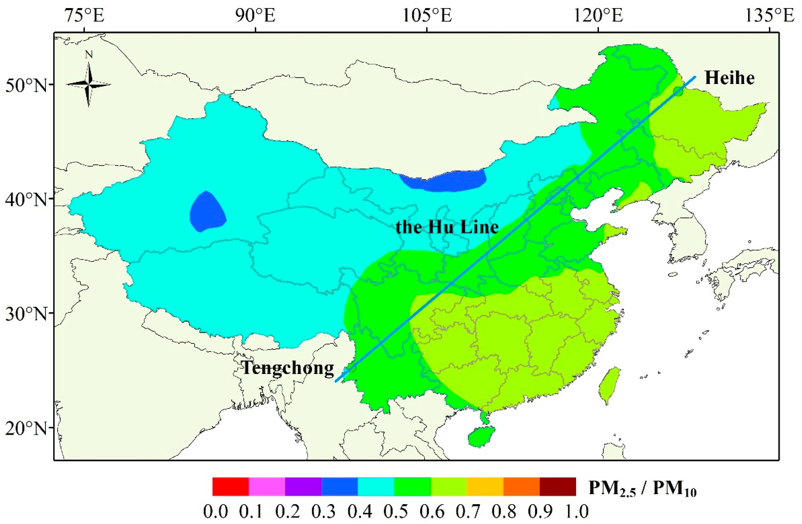
  26. Hu, H. The distribution of population in China. Acta Geogr. Sin. 1935, 2, 33–74. [Google Scholar]
  27. Wang, S.; Zhou, C.; Wang, Z.; Feng, K.; Hubacek, K. The characteristics and drivers of fine particulate matter (PM2.5) distribution in China. J. Clean. Prod. 2017, 142, 1800–1809. [Google Scholar] [CrossRef]
  28. Zhang, H.; Wang, Y.; Hu, J.; Ying, Q.; Hu, X.M. Relationships between meteorological parameters and criteria air pollutants in three megacities in China. Environ. Res. 2015, 140, 242–254. [Google Scholar] [CrossRef] [PubMed]
  29. Jian, L.; Zhao, Y.; Zhu, Y.P.; Zhang, M.B.; Bertolatti, D. An application of ARIMA model to predict submicron particle concentrations from meteorological factors at a busy roadside in Hangzhou, China. Sci. Total Environ. 2012, 426, 336–345. [Google Scholar] [CrossRef] [PubMed]
  30. Li, X.; Liu, W.; Chen, Z.; Zeng, G.; Hu, C.; León, T.; Liang, J.; Huang, G.; Gao, Z.; Li, Z.; et al. The application of semicircular-buffer-based land use regression models incorporating wind direction in predicting quarterly NO2 and PM10 concentrations. Atmos. Environ. 2015, 103, 18–24. [Google Scholar] [CrossRef]
  31. Qin, S.; Liu, F.; Wang, J.; Sun, B. Analysis and forecasting of the particulate matter (PM) concentration levels over four major cities of China using hybrid models. Atmos. Environ. 2014, 98, 665–675. [Google Scholar] [CrossRef]
  32. Price, D.T.; Mckenney, D.W.; Nalder, I.A.; Hutchinson, M.F.; Kesteven, J.L. A comparison of two statistical methods for spatial interpolation of Canadian monthly mean climate data. Agric. For. Meteorol. 2000, 101, 81–94. [Google Scholar] [CrossRef]
  33. Houghton, J.T. Climate change 1995: The science of climate change. Clim. Chang. 1996, 67, 1261. [Google Scholar]
  34. Atkinson, P.M.; Lloyd, C.D. Mapping precipitation in Switzerland with ordinary and indicator Kriging. J. Geogr. Inform. Decis. Anal. 1998, 2, 65–76. [Google Scholar]
  35. Liu, W.; Li, X.; Chen, Z.; Zeng, G.; León, T.; Liang, J.; Huang, G.; Gao, Z.; Jiao, S.; He, X.; et al. Land use regression models coupled with meteorology to model spatial and temporal variability of NO2 and PM10 in Changsha, China. Atmos. Environ. 2015, 116, 272–280. [Google Scholar] [CrossRef]
  36. Li, X.; Gao, Z.; Chen, Z.; Zeng, G.; León, T.; Liang, J.; Li, F.; Liu, W.; Wu, H.; Du, C.; et al. Eutrophication research of Dongting Lake: An integrated ML-SEM with neural network approach. Int. J. Environ. Pollut. 2017, 62, 31–52. [Google Scholar] [CrossRef]
  37. Elith, J.; Leathwick, J.R.; Hastie, T. A working guide to boosted regression trees. J. Anim. Ecol. 2008, 77, 802–813. [Google Scholar] [CrossRef] [PubMed]
  38. Zhang, W.; Du, Z.; Zhang, D.; Yu, S.; Hao, Y. Boosted regression tree model-based assessment of the impacts of meteorological drivers of hand, foot and mouth disease in Guangdong, China. Sci. Total Environ. 2016, 553, 366–371. [Google Scholar] [CrossRef] [PubMed]
  39. Ridgeway, G. Gbm: Generalized Boosted Regression Models. R Package Version 1.6-3.2. 2012. Available online: https://cran.r-project.org/ (accessed on 14 December 2017).
  40. Sayegh, A.; Tate, J.E.; Ropkins, K. Understanding how roadside concentrations of NOx are influenced by the background levels, traffic density, and meteorological conditions using Boosted Regression Trees. Atmos. Environ. 2016, 127, 163–175. [Google Scholar] [CrossRef]
  41. Carslaw, D.C.; Taylor, P.J. Analysis of air pollution data at a mixed source location using boosted regression trees. Atmos. Environ. 2009, 43, 3563–3570. [Google Scholar] [CrossRef]
  42. Wang, J.F.; Xu, C.D.; Tong, S.L.; Chen, H.Y.; Yang, W.Z. Spatial dynamic patterns of hand-foot-mouth disease in the People’s Republic of China. Geospat. Health 2013, 7, 381–390. [Google Scholar] [CrossRef] [PubMed]
  43. Zhang, W.; Du, Z.; Zhang, D.; Yu, S.; Hao, Y. Quantifying the adverse effect of excessive heat on children: An elevated risk of hand, foot and mouth disease in hot days. Sci. Total Environ. 2016, 541, 194–199. [Google Scholar] [CrossRef] [PubMed]
  44. Zhang, W.; Yuan, S.; Hu, N.; Lou, Y.; Wang, S. Predicting soil fauna effect on plant litter decomposition by using boosted regression trees. Soil Biol. Biochem. 2015, 82, 81–86. [Google Scholar] [CrossRef]
  45. Hastie, T.; Tibshirani, R.; Friedman, J. The Elements of Statistical Learning: Data Mining, Inference, and Prediction; Springer: New York, NY, USA, 2001. [Google Scholar]
  46. Ministry of Environmental Protection of the People’s Republic of China. Ambient Air Quality Standards (GB 3095-2012); Ministry of Environmental Protection of the People’s Republic of China: Beijing, China, 2012.
  47. Huang, R.J.; Zhang, Y.; Bozzetti, C.; Ho, K.F.; Cao, J.J.; Han, Y.; Daellenbach, K.R.; Slowik, J.G.; Platt, S.M.; Canonaco, F.; et al. High secondary aerosol contribution to particulate pollution during haze events in China. Nature 2014, 514, 218–222. [Google Scholar] [CrossRef] [PubMed] [Green Version]
  48. Cao, C.; Lee, X.; Liu, S.; Schultz, N.; Xiao, W.; Zhang, M.; Zhao, L. Urban heat islands in China enhanced by haze pollution. Nat. Commun. 2016, 7, 12509. [Google Scholar] [CrossRef] [PubMed]
  49. Yang, L.; Zhang, F.; Gao, Q.; Mao, R.; Liu, X. Impact of land-use types on soil nitrogen net mineralization in the sandstorm and water source area of Beijing, China. Catena 2010, 82, 15–22. [Google Scholar] [CrossRef]
  50. Zeng, X.; Zhang, W.; Cao, J.; Liu, X.; Shen, H.; Zhao, X. Changes in soil organic carbon, nitrogen, phosphorus, and bulk density after afforestation of the “Beijing–Tianjin Sandstorm Source Control” program in China. Catena 2014, 118, 186–194. [Google Scholar] [CrossRef]
  51. Wang, Z. The impacts of climate on the society of China during historical times. Acta Geogr. Sin. 1996, 51, 329–339. [Google Scholar]
  52. Hu, J.; Wu, L.; Zheng, B.; Zhang, Q.; He, K.; Chang, Q.; Li, X.; Yang, F.; Ying, Q.; Zhang, H. Source contributions and regional transport of primary particulate matter in China. Environ. Pollut. 2015, 207, 31–42. [Google Scholar] [CrossRef] [PubMed]
  53. Wang, Q.; Huang, R.-J.; Cao, J.; Tie, X.; Shen, Z.; Zhao, S.; Han, Y.; Li, G.; Li, Z.; Ni, H.; et al. Contribution of regional transport to the black carbon aerosol during winter haze period in Beijing. Atmos. Environ. 2016, 132, 11–18. [Google Scholar] [CrossRef]
  54. Zhang, X.Q.; McMurray, P.H.; Hering, S.V.; Casuccio, G.S. Mixing characteristics and water content of submicron aerosols measured in Los Angeles and at the grand canyon. Atmos. Environ. Part A Gen. Top. 1993, 27, 1593–1607. [Google Scholar] [CrossRef]
  55. Kasper, A.; Puxbaum, H. Seasonal variation of SO2, HNO3, NH3 and selected aerosol components at Sonnblick (3106 m a.s.l.). Atmos. Environ. 1998, 32, 3925–3939. [Google Scholar] [CrossRef]
  56. Yu, L.; Wang, G.; Zhang, R.; Zhang, L.; Song, Y.; Wu, B.; Li, X.; An, K.; Chu, J. Characterization and Source Apportionment of PM2.5 in an Urban Environment in Beijing. Aerosol Air Qual. Res. 2013, 13, 574–583. [Google Scholar] [CrossRef]
Figure 1. Locations of the 173 monitored cities in China.
Sustainability 09 02330 g001
Figure 2. Box plot of five meteorological elements. A Box-and-Whisker Plot includes such parts: the mean (denoted by a square), the median (denoted by a horizontal bar in the box), the 25th percentile (denoted by the bottom edge of the box), the 75th percentile (denoted by the top edge of the box), the 5 percentiles (denoted by the bottom edge of the whisker), the 95 percentiles (denoted by the top edge of the whisker), and the dots denote the data distribution.
Sustainability 09 02330 g002
Figure 3. Maps of the spatial change in the annual average of PM2.5 and PM10 concentrations in China. The left sloping blue line marks the Hu Line, which is a boundary line of the distribution of Chinese population on the map of China. The right blue curve line marks the Yangtze River, which is the third longest river in the world.
Sustainability 09 02330 g003
Figure 4. Statistical difference of PM2.5 and PM10 divided respectively by the Hu Line and the Yangtze River. Note: SEH represents the cities situated southeast of the Hu Line, NWH represents the cities situated northwest of the Hu Line, NY represents the cities located north of the Yangtze River and SY represents the cities located south of the Yangtze River. A Box-and-Whisker Plot details the mean (denoted by a square), the median (denoted by a horizontal bar in the box), the 25th percentile (denoted by the bottom edge of the box), the 75th percentile (denoted by the top edge of the box), the 5 percentiles (denoted by the bottom edge of the whisker), the 95 percentiles (denoted by the top edge of the whisker), and the dots denote the data distribution.
Sustainability 09 02330 g004
Figure 5. Ratio of annual average PM2.5 concentrations to annual average PM10 concentrations in China.
Sustainability 09 02330 g005
Figure 6. Maps of spatial distribution in the considered meteorological factors: precipitation, relative humidity, temperature, pressure, and wind speed. Precipitation is the total amount over an entire year. The remaining meteorological factors are the calculated annual average values.
Sustainability 09 02330 g006
Figure 7. Relative contributions of each meteorological variable to the spatial distribution of PM2.5 and PM10 by the boosted regression tree analysis. Note: VE, verification; CV, cross validation; SE, standard error.
Sustainability 09 02330 g007
Figure 8. Relationships between PM with meteorological elements based on the spatial characteristics. Rug plots at inside top of plots indicate distribution of sites across that variable, in deciles. In the plots, TEM, PREC, PRES, WS, and HUM indicate temperature, precipitation, pressure, wind speed, and relative humidity, respectively.
Sustainability 09 02330 g008

