A Hybrid Local Search Algorithm for the Sequence Dependent Setup Times Flowshop Scheduling Problem with Makespan Criterion


1
School of Information and Science Technology, Northeast Normal University, Changchun 130117, China
2
Department of Computer Science, College of Humanities & Sciences of Northeast Normal University, Changchun 130117, China
*
Authors to whom correspondence should be addressed.
Sustainability 2017, 9(12), 2318; https://doi.org/10.3390/su9122318
Submission received: 25 October 2017
/
Revised: 7 December 2017
/
Accepted: 9 December 2017
/
Published: 14 December 2017
Abstract
:This paper focuses on the flowshop scheduling problem with sequence dependent setup times (FSSP-SDST), which has been an investigated object for decades as one of the most popular scheduling problems in manufacturing systems. A novel hybrid local search algorithm called HLS is presented to solve the flowshop scheduling problem with sequence dependent setup times with the criterion of minimizing the makespan. Firstly, the population is initialized by the Nawaz-Enscore-Hoam based problem-specific method (NEHBPS) to generate high quality individuals of the current population. Then, a global search embedded with a light perturbation is designed to produce a new population. After that, to improve the quality of individuals in the current population, a single insertion-based local search is applied. Meanwhile, a further local search strategy based on the insertion-based local search is used to find better solutions for the individuals which are non-improved. Finally, the heavy perturbation is used to explore potential solutions in the neighbor region. To validate the performance of HLS, we compare our proposed algorithm with other competitive algorithms on Taillard benchmark problems. From the experimental results, it can be concluded that the proposed algorithm outperforms the benchmark algorithms.
1. Introduction
Permutation flowshop scheduling is one of the classical combinatorial optimization problems since the seminal work of Johnson Seminal [1], which is widely applied in real life, such as computer work, industrial engineering, mathematics. In particular, the permutation flowshop scheduling problem with sequence dependent setup times has attracted the attention of many researchers. For this problem, the sequence dependent means that the setup times of the processing jobs depend both on the preceding job and the job to be processed. It is different from the sequence independent which depends only on the job to be processed [2,3]. Meanwhile, the setup time is regarded as negligible in a lot of cases thus it is often ignored or dealt with a part of processing time [4,5,6,7].
Recently, many heuristic methods have been introduced to solve this problem since exact methods [8] may take too much computation cost. However, the exact methods are applied widely in the hybridization algorithms for many combinational optimization problems. Such as, Nishi and Hiranaka employed the Lagrangian relaxation and cut generation technique for solving sequence-dependent setup time flowshop scheduling problems to minimise the total weighted tardiness effectively [9], and in the book about the use of metaheuristics in optimization [10], the chapters [11,12] surveyed the integer linear programming techniques and metaheuristics derived from branch and bound for the combinatorial optimization respectively. Furthermore, Andreagiovanni and Nardin [13] proposed an improved ant-colony algorithm for designing sensor networks in 2015, where linear programming relaxations were employed to take better variable fixing decisions. Andreagiovanni and et al. also raised a very effective and fast algorithm [14] integrated an ant colony-like algorithm with an approximation algorithm and linear relaxations for solving multiperiod network design. Besides, Gambardella and et al. [15] presented how ant colony algorithms combined with solution improvement phases following some simple but effective rules can lead to good improvements in the quality of obtained solutions. In terms of the heuristic algorithms, the advantage of them is that some excellent solutions can be gained quickly, contrarily the disadvantage is that the quality of the solutions can not be guaranteed in general. There are three types of heuristics including constructive heuristic, meta-heuristic and hybrid heuristic respectively to deal with FSSP-SDST in the literature. A constructive heuristic comprises a stochastic construction and a greedy construction, and constructs feasible solutions by adding jobs one by one to the partial permutation. NEH algorithm was proposed by Nawaz et al. [16] and proved effective in finding the good solution for FSSP-SDST. Based on it, Rios-Mercado and Bard [17] proposed an extension constructive deterministic heuristic (NEHT_RMB) with high effectiveness for FSSP-SDST with the makespan objective. Meanwhile, a greedy randomized adaptive search procedure (GRASP) was also presented to improve the fitness of solutions. Ruiz et al. [18] used two algorithms namely a novel genetic algorithm (GA) and a memetic algorithm (MA) based on the classical genetic algorithm and they performed better than that of Rios-Mercado and Bard [19]. Rajendran and Ziegler [20] proposed an ant colony optimization (PACO) to enhance the solutions for FSSP-SDST with the objective of makespan and total flowtime of jobs respectively using NEHT_RMB method. Another ant colony optimization algorithm (ACO) was developed by Gajpal et al. [21] for FSSP-SDST with makespan criterion. Tseng et al. [22] presented an inventive heuristic algorithm and compared it with an existing index heuristic algorithm. The migrating birds optimization meta-heuristic was proposed by Benkalai et al. [23] and its good performance was proved by related experiments. The last but not least type of the heuristic is the hybrid algorithm; it also contains many algorithms blended with local search methods. Rios-Mercado and Bard [19] developed a heuristic algorithm called the hybrid algorithm which was the modification of the four heuristics compared with three benchmarks presented by Simons [24]. Besides, a new heuristic method called iterative greedy algorithm (IG) was proposed by Jacobs and Brusco [25], which was applied widely in other heuristics and had shown better performance for FSSP-SDST in the algorithm developed by Ruiz et al. [26]. Based on the basic IG (IG_RS), an effective local search was added to it in the destruction and construction phases for FSSP-SDST. In the same way, that effective local search was also added to the original MA which was called MA to solve the same problem. By the experiments, it has to be noted that the above two hybrid algorithms, IG_RS and MA, outperformed others including earlier heuristics and that of Rajendran and Ziegler [27] in getting better solutions. In addition, another effective iterated local search algorithm (ILS) developed by Wang et al. was shown its high efficiency with the objective of makespan in FSSP-SDST [28]. However, most of the above algorithms still cannot find solutions with high quality in a reasonable computational time. In this paper, we propose a hybrid local search algorithm for the sequence dependent setup times flowshop scheduling problem with makespan criterion. The difference of our proposed algorithm is that in most of the above algorithms, the initial individuals are generated randomly to keep the diversity of the population and most of them are not of high quality and this leads to solutions of low quality in next generations. In HLS, a NEH based problem-specific method is applied to guarantee the diversity and quality of the initial solutions at the same time. Besides, some of the above methods only focus on the global search capability and on contrary close attention to the local search ability is paid in some algorithms such as ILS and ACO. Hence, we combine the global search with the local search to enhance the solution quality in HLS. Furthermore, without effective perturbation methods, some algorithms such as IG_RS and IG_RS, are easy to be trapped into a local optimum after a number of iterations of local search without improving the quality of solutions further. Thus, in HLS, an efficient perturbation method is carried out to guide the search towards another area of the solutions and achieve better exploration.
Based on the above analyses, the hybrid local search algorithm can be summarized as follows: first of all, an overall framework of HLS based on local search and perturbation operators is presented to solve FSSP-SDST. During the search, the NEH based problem-specific method is used to initialize the population. Then to improve the performance of current population, a global search with a perturbation is applied. Next, we use an insertion-based local search to enhance the solutions for FSSP-SDST. What’s more, a further local search method is used to exploit neighbors with good quality if the individuals cannot be improved by single local search method. At last, an update method is applied to update the current population. In order to show the performance of our proposed algorithm, six state-of-the-art algorithms namely GA, MA, MA, IG_RS, IG_RS and PACO are compared to test its high effectiveness. For the purpose of experimentation, we use the Taillard benchmark problems for FSSP-SDST at four levels including SDST10, SDST50, SDST100 and SDST125 with 12 sizes of data to analyze the performance of all the above seven algorithms. The statistical results show the high efficiency and competitive performance of HLS.
The rest of this paper is organized as follows: Section 2 describes the flowshop scheduling problem with sequence dependent setup times. The detail of the proposed algorithm is given in Section 3. In Section 4, the computational experiments are conducted. Finally, we draw the conclusion and the future work in Section 5.
2. The Flowshop Scheduling Problem with Sequence Dependent Setup Times
For the flowshop scheduling problem with sequence dependent setup times, a set of n jobs or tasks in J = {1, 2, 3, …, n} has to be processed on a set M = {1, 2, 3, …, m} of m machines sequentially, such as first on machine 1, then on machine 2, till the end on machine m. The objective of this problem is to find a processing sequence with the minimized makespan ). For all the machines, the operating order of each processing sequence is identical. For a job permutation sequence , the value of the setup times depends on the current job processing on the certain machine and the next job in the same permutation. Each job can be processed on one machine every time and meanwhile each machine can process only one job. All operations are non-preemptive and none of them on each machine has the priority. The definition of the flowshop scheduling problem with sequence dependent setup times can be described as follows:
where is denoted as the setup time when producing job on the machine j after having processed job . denotes the processing time of job on machine j. The is the complete time of job on machine j. In this paper, we assume that , and .
3. A Hybrid Local Search Algorithm
3.1. Overall Framework
In this section, the hybrid local search framework for solving FSSP-SDST with the objective of makespan is proposed by integrating some problem-specific methods. Each operator plays an important role in improving the efficiency of HLS.
At the beginning of the proposed algorithm, a NEH based problem-specific heuristic is utilized to initialize the population with N individuals. In other words, N permutation sequences for FSSP-SDST are formed. Then an improved population with good neighbor individuals is developed by the global search method. In addition, an effective single insertion-based local search method is applied to each individual for exploiting good individuals around it. If a better individual is found, the previous one will be updated. Otherwise, the multiple insertion-based local search is executed deeply as a further search regarding the individuals that are trapped into the local optima. Then, the solution will be stored in PotentialInd to maintain the good individual completely. In order to explore individuals transversely, the heavy perturbation approach is used to partly guide the trend of search. At last, we apply an effective update method to update the current population. The detail schemes of HLS are given in Algorithm 1.
| Algorithm 1 HLS. |
| Input: |
| The population size N. |
| The number of jobs n. |
| The maximum times of further search FSNum. |
| Output: |
The best individual .
|
3.2. Initialization
Regarding the initialization stage, it is divided into three parts including the population initialization, PotentialInd initialization and the initialization of . First, for the population initialization, it is generated randomly. Then, in order to produce some high quality solutions, the NEH based problem-specific method is applied to initialize the population which is composed of N random individuals. After that, HLS can provide some high quality solutions at the beginning of the search process. NEH method can be presented as follows in detail:
- (1)
- Select a solution s from randomly, the first two jobs are extracted and two partial possible schedules with these two jobs are evaluated. The better one based on makespan is chosen as the current sequence.
- (2)
- For each unscheduled job j in s, put it into all the possible positions of the current scheduled sequence to generate all the possible partial sequences. The best one is selected as the current sequence for scheduling the next job.
- (3)
- A new individual is formed after scheduling all jobs, if is better than s, then it will replace s.
With respect to NEHBPS, for N times of iterations, a random individual is chosen to carry out NEH. Not all the individuals are processed by NEH, hence, the diversity of the initial population can be ensured. In summary, a population is generated with the feature of quality and diversity.
Secondly, HLS will initialize PotentialInd by assigning it a determinate sequence to store some problem-specific heuristic information. It is promised that a good individual is stored completely to get ready for finding the best individual during the search process.
Lastly, we initialize using the first individual in the population. This individual is updated via the iterations of search process in HLS. At the end of HLS, will be outputted with the minimum makespan for FSSP-SDST.
3.3. Global Search Method
The goal of this method is to gain an improved population by perturbing the good individuals and then updating them. In this subsection, the top 25% individuals are chosen as a new elite population to carry out the light perturbation. This setting aims to explore large search space using the appropriate solutions. Furthermore, we update the current population by using the individual which has undergone the light perturbation for enhancing the fitness of the population overall. The framework of GlobalSearch is shown in Algorithm 2.
| Algorithm 2 GlobalSearch. |
| Input: |
| The number of jobs n. |
| The current population . |
| The maximal number of GlobalSearch GSNum. |
| The mutation probability . |
| Output: |
The improved population .
|
This method allows the perturbed solution to maintain some characteristics of the previous solution and find other characteristics in new solutions for improving the diversity of the population. It also helps HLS to find other optimal solutions in the neighborhoods. The light perturbation strength is so sufficient to lead the search trajectory to another neighbor region which can result in a different solution. In conclusion, GlobalSearch can both enhance the diversity of the population and improve the convergence rate of HLS.
3.4. Update Method
In this section, two algorithms, namely Algorithms 3 and 4, are presented. In Algorithm 3, we use the specified individual to update the individual randomly in the current population. At the same time, the update population method is presented in Algorithm 4. After achieving it, an elite population including some individuals with top fitness has acquired.
| Algorithm 3 UpdateInds. |
| Input: |
| The current population . |
| An individual to be used for updating s. |
| Output: |
The current population with updated individuals .
|
| Algorithm 4 UpdateP. |
| Input: |
| The population size N. |
| Each individual in the current population . |
| The maximal update number UpdateNum. |
| Output: |
The updated population .
|
Except for the above two update methods, another update method is used for PotentialInd. As Algorithm 1 dedicates, if the current solution has improved successfully in the single insertion-based local search or the further search section, PotentialInd will be updated.
3.5. Perturbation and Local Search Methods
In the single insertion-based local search and the further search, if the current individual has been replaced with a better individual, then the better one is stored. Otherwise, it means that this solution has been trapped into a local optimum, the heavy perturbation will be employed to the current solution. Compared with the light perturbation, the heavy perturbation has larger interference strength to provide enough perturbation for the high quality solutions. The heavy perturbation is used to obtain some characteristics of the previous solution, but it isn’t apt for all the local search methods. Such as in GlobalSearch, the light perturbation method is more suitable as it has a better result for disturbing the good solution with the relatively fitting strength. The light perturbation and the heavy perturbation operations can be defined as follows:
- The heavy perturbation:
- (1)
- Input a solution s. Three different positions of s are randomly selected, where .
- (2)
- Let represent the partial sequence between and and denote the other partial sequence between and (not including ), then exchange and to generate a new solution to be outputted.
- The light perturbation:
- (1)
- Input a solution s. Two different positions of s are randomly selected, where .
- (2)
- Let S represent the partial sequence between and (not including ), then move the job in position behind S to generate a new solution to be outputted.
On the first phase, a single insertion-based local search is employed to HLS for exploring better solutions. In [29,30,31,32,33,34,35,36,37], this local search has shown its high effectiveness in obtaining the better quality solutions than the local search based on swap operators. The curial idea of this method is to compare the previous makespan with the new makespan of the sequence, which has inserted a job into all positions of the sequence. Then the better one will be accepted. But if a solution cannot be improved, it will experience the further search to make it rope out of the local optimum on the second phase. Moreover, the further search with the purpose of exploiting good individuals in the neighborhood can increase the convergence speed of HLS. The effective insertion-based local search is described as follows:
- (1)
- Input a solution s and a position r.
- (2)
- Let the job j be a job in the position r. Put j into each of the left possible positions of s to generate neighborhood solutions.
- (3)
- Let be the best solution based on the minimal makespan among the neighborhood solutions.
- (4)
- Output .
3.6. How to Balance between Exploitation and Exploration
For designing the hybrid heuristic algorithm, it is known to all that diversity and convergence are the two basic issues. In terms of diversity, exploitation is executed in HLS for improving the convergence rate. Otherwise, explorations to other search directions on breadth is applied to HLS for maintaining or enhancing the diversity of the population. HLS can trade off the convergence and diversity efficiently where the diversity is pursued by the exploration and the convergence is increased in the manner of the exploitation.
- (1)
- Regarding the exploitation: It means that a further search in the large and deep search space can be executed. For the purpose of searching better solutions, firstly we have used the single insertion-based local search to begin the evolution of population. Furthermore, if the current individual cannot be replaced with the new one after carrying out the single local search, thus secondly we choose the further search based on the insertion-based local search to search the solutions deeply. After above methods, the rate of convergence can be improved quickly.
- (2)
- Regarding the exploration: In other words, the central idea of it is to maintain the diversity of the population. In the search process, we have applied the heavy perturbation method to the individuals which are trapped in the local optima. This way effectively avoids the current population being trapped into the local optima and urges that population to an anticipant direction for next generation. It is particularly worth mentioning here that the light perturbation in GlobalSearch keeps the diversity of the improved population, which has a high convergence for searching good solutions at the same time.
As we expect, a good population with high quality and diversity will be formed. Moreover, at the foundation of the above analyses, HLS can balance the exploitation with exploration in the search process successfully.
4. Experimental Results
4.1. Environmental Setup
HLS is performed on a PC with 4 GB RAM and a CPU of 3.40 GHz on Windows 7 OS. It is programmed in C++ by Microsoft Visual Studio 2013. It is obviously known that the algorithm with the more running time can bring out the better result. To compare with other algorithms fairly, the stop criterion of HLS is CPU time limit given by milliseconds. Besides, f is set as 30, 60, 90 respectively, which is the same as Ruiz used in [38].
4.2. Benchmark Problem Instances and Benchmark Algorithms
To verify the performance of the proposed algorithm, Taillard-based sets from Vallada et al. (2003) including 4 sets and 480 benchmark instances are used. The instances in each set range from 20 jobs with 5 machines to 500 jobs with 20 machines, consisting of 20 × 5, 20 × 10, 20 × 20, 50 × 5, 50 × 10, 50 × 20, 100 × 5, 100 × 10, 100 × 20, 200 × 10, 200 × 20 and 500 × 20 respectively. Besides, each size has 10 specific examples. It’s remarkable that each set is different in processing times and setup times. The first two sets are SDST10 and SDST50, in which the setup times are 10% and 50% of the average processing times . In other words, the setup times are generated equably from the distribution ranges [1, 9] and [1, 49] because in this benchmark are uniformly generated in the distribution range [0, 99]. Similarly, the last two sets are SDST100 and SDST125, in which the setup times are generated uniformly from the distribution ranges [1, 99] and [1, 124], respectively 100% and 125% of .
Then, to show the effectiveness of HLS, six efficient algorithms including GA, MA, MA, PACO, IG_RS, and IG_RS on FSSP-SDST [18,38] are used to compare with our proposed algorithm. Furthermore, a response variable called the relative percentage deviation (RPD) is applied to show the increase between a specific solution produced from a certain algorithm and the best bound found in http://soa.iti.es/problem-instances.
4.3. Experimental Parameter Settings
HLS has five control parameters, comprised of N, , GSNum, UpdateNum and FSNum. Instances Ta071–Ta080 () in SDST50 are used to calibrate the parameters as the base case due to space limitations in the following experiments. Each experiment runs ten times independently with CPU time equaling to . The good results relatively are marked in bold.
4.3.1. The Influence of the Population Size N
It is obvious that the population size is an essential parameter to heuristic algorithms. Selecting an appropriate size has been known as a challenging and puzzling task. If the size is too small, it is easy for the algorithm to have a fast convergence which leads to local optima prematurely. However, using too large size will bring about additional computation costs. To get the influence of the population size on the search performance distinctly, the population size has been varied from 10 to 40 with the RPD results summarized in Table 3.
From the average results of RPD in Table 3, the population size 20 can provide better average RPD (ARPD) in some instances including Ta071, Ta075, Ta078 and Ta080. In Ta078, a population size 10 provides the same least ARPD as a population size 20 with the value of 0.41. Besides a population size 10 and 30 can bring out the same least ARPD (0.56) in Ta079. Moreover, HLS with a population size 30 can gain a better RPD in instances Ta074, Ta077 and Ta079. Figure 2 gives an empirical insight of influence on each population size using the confidence intervals at the 95% confidence level of ARPD for Ta071–Ta080 and it is observed that the population size 20 beats other settings with the best ARPD. Therefore, it is concluded that the population size 20 outperforms other settings in producing better ARPD results.
4.3.2. The Influence of the Maximal Number of GlobalSearch GSNum
In this experiment, we will discuss the effect of GSNum. In GlobalSearch, GSNum indicates the maximum number of iterations that conduct the search on the selected individuals who can be further interfered. To demonstrate the effect of GSNum on the proposed algorithm, Ta071–Ta080 are also applied to present the performance measured as RPD with GSNum chosen from set {3, 4, 5, 6}. Other parameters temporarily set as the previous experiment in this experiment. Table 4 summaries RPD results of each GSNum.
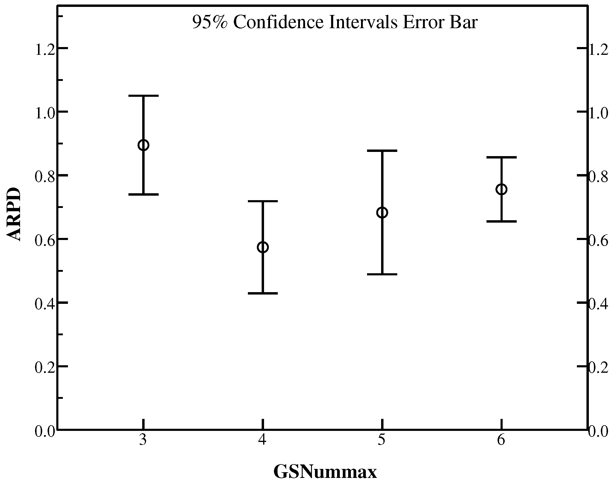
From Table 4, it is easily observed that GSNum = 3 gains only one best result in Ta071, while GSNum = 4 can perform better in Ta075, Ta076, Ta078, Ta079 and Ta080. What’s more, GSNum = 5 provides better results on three instances including Ta073, Ta074 and Ta077, however only in Ta072, GSNum = 6 beats other settings. In general, GSNum = 4 gives the best average RPD on instance set Ta071–Ta080.
Figure 3 provides the 95% confidence interval error graph in terms of ARPD for Ta071–Ta080 with different GSNum. We can find that GSNum = 4 has a strong adaptability with higher convergence ability and it is good in solving FSSP-SDST with the best ARPD among all the settings. Based on the above analyses, it is summarized that GSNum = 4 results in the better performance for most instances in terms of RPD. Therefore, GSNum = 4 is the best choice for HLS.
4.3.3. The Effect of the Mutation Probability
As HLS introduced before, in GlobalSearch, a mutation probability was used to control iteration times to implement the perturbation and update process. It is so important that too large will bring a move at angles to the space with better results and small values of will guide the search to the parallel axes in the exploring space. Hence, a set of ranging from 0.1 to 0.4 is used to present the relative performance in getting better results with Ta071–Ta080. Table 5 details the results with different values of .
It is shown in Table 5 that = 0.1 can gain best RPD only in Ta075, while = 0.2 provides better RPD in instances set Ta071, Ta074. Besides, = 0.3 can give better results in most of the instances including Ta072, Ta073, Ta076, Ta079 and Ta080 with the smallest average RPD. For Ta077 and Ta078, = 0.4 performs better results among all the settings. ARPD concluded in average 95% CI is presented in Figure 4. Generally speaking, the experiments implies that = 0.3 might be a good setting to solve FSSP-SDST with the better ARPD.
4.3.4. The Influence of the Maximal Number of Update UpdateNum
In the update method UpdateP of HLS, we use UpdateNum to present the maximal iteration number of update taking advantage of an individual separately. To maintain the diversity of the population, the value of it can’t be too large and it should be less than the population size N according to the framework of UpdateP, however if it was too small, the update method has little effect on gaining better result in the search space. A certain number is not apt for all instances. Here UpdateNum is set as 4, 6, 8, 10 to test its suitability. Other settings are as the preliminary experiments. Table 6 shows the detail results.
From Table 6, UpdateNum = 4 is suitable for Ta072, Ta073, Ta079 and Ta080. For Ta071, Ta074 and Ta077, UpdateNum = 6 beats others in getting better RPD. By the same way, Ta072 and Ta075 can give better results when UpdateNum = 8 while UpdateNum = 10 provides better RPD in instances Ta076 and Ta078. Herein UpdateNum = 4 and UpdateNum = 8 present the same results in Ta072. As can be seen in the average RPD, UpdateNum = 6 outperforms other numbers of UpdateNum. It can be found in Figure 5, an average RPD plot with the confidence intervals at the 95% confidence level is shown and it is easy to find out that UpdateNum = 6 performs best among all the settings. There can be concluded that different numbers of UpdateNum will affect the performance of the proposed algorithm variously and we set UpdateNum to 6 for its good achivement.
4.3.5. The Effect of the Maximum Number of Further Search FSNum
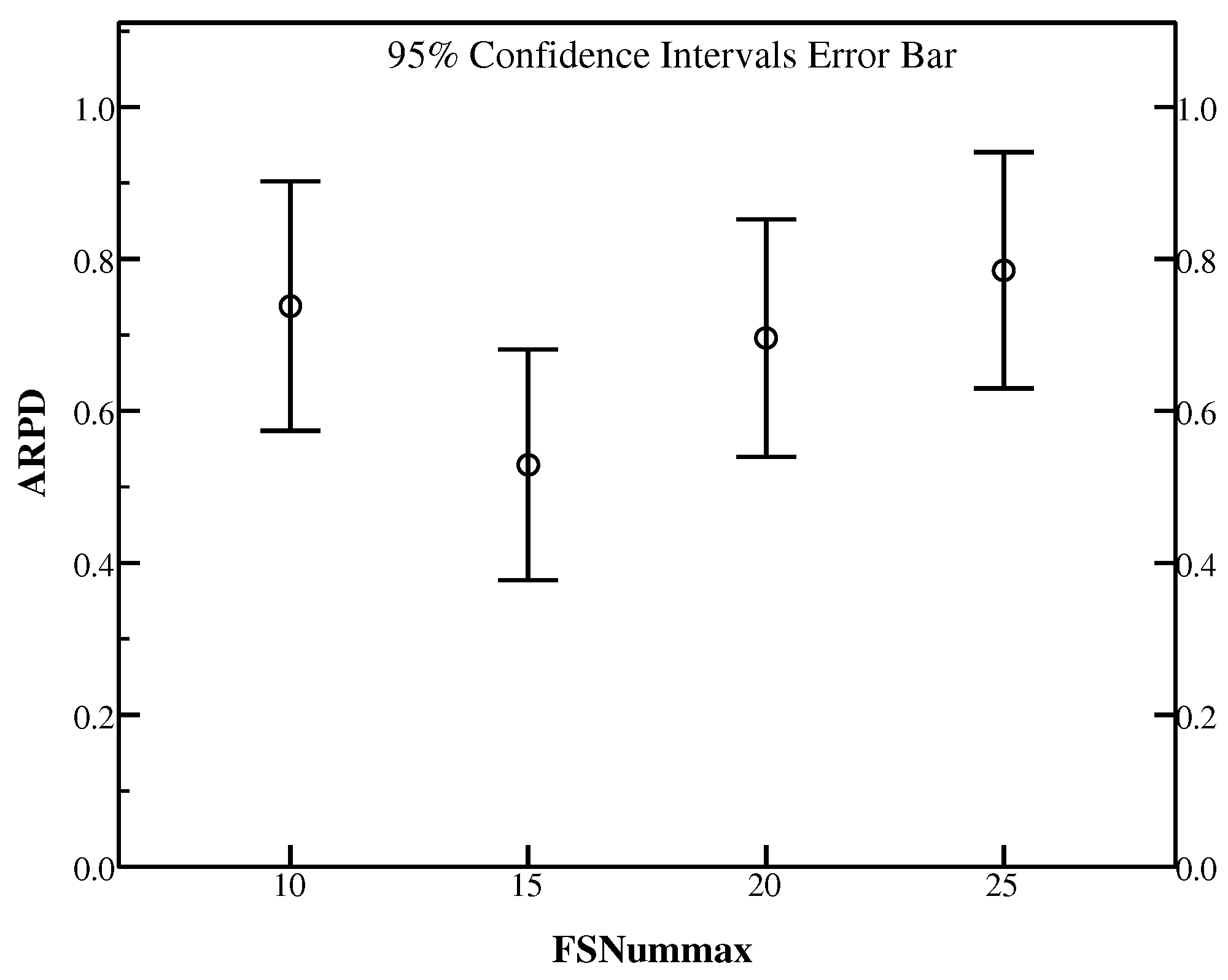
If some individuals cannot be improved in the single insertion-based local search, then a further search method will be applied to them. In this section, the effect of FSNum used to define the maximal number of the further exploitation will be discussed. We have taken advantage of Ta071–Ta080 measured as RPD to present the effect. The value of it varies through the set {10, 15, 20, 25} and other parameter settings are the same as the previous experiments. The results of the settings are summarized in Table 7.
From Table 7, FSNum = 10 provides good RPD on Ta072, however for Ta078 and Ta073, FSNum = 20 and FSNum = 25 perform better than other settings respectively. For the rest instances including Ta071, Ta074, Ta075, Ta076, Ta077, Ta079 and Ta080, FSNum = 15 is a good setting beating other values in gaining better RPD. It is obvious that FSNum = 15 outperforms others on most of the instances. Besides, Figure 6 demonstrates ARPD with 95% confidence interval of all the ten instances. It can be easily seen that FSNum = 15 has the best result for solving the instances in HLS.
4.4. Effect of NEH Based Problem-Specific Heuristic
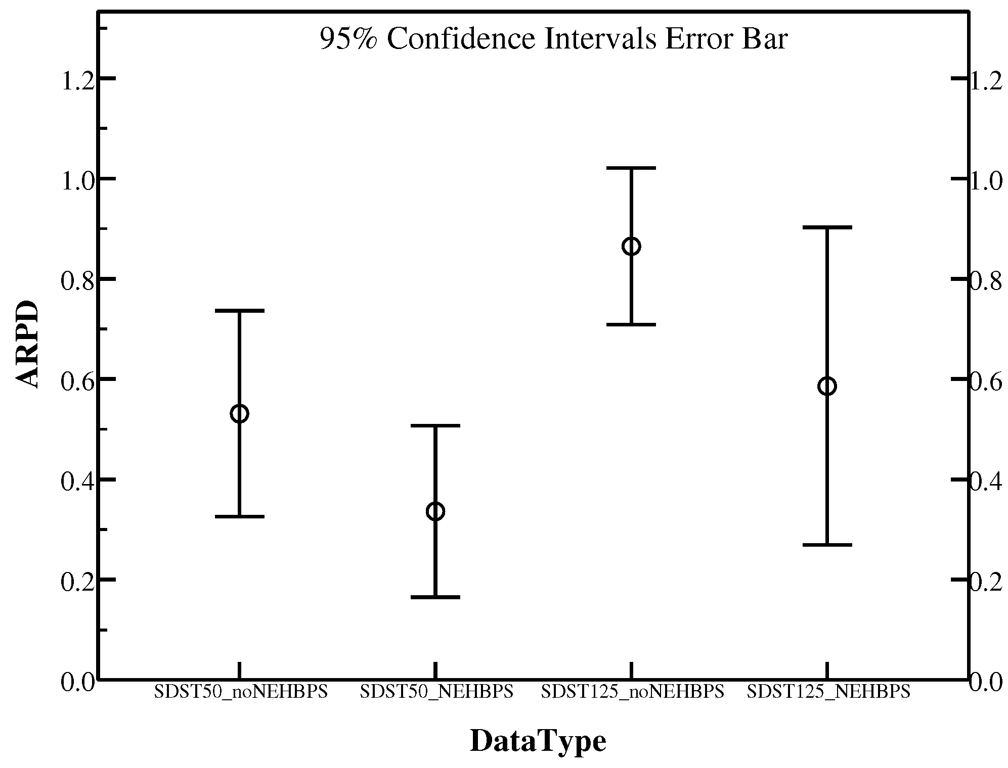
In the initial stage of the proposed algorithm, a NEH based problem-specific heuristic method is used to initialize the population which is produced by a random method. It plays an important part in enhancing the results of the algorithm. Without it, the search of getting good individuals will spread out in a quite broad direction. We respectively use the instances Ta071–Ta080 () in SDST50 and SDST125 ran ten times to demonstrate the vital effect of it. Besides, the rest frameworks are the same in order to compare fairly. Table 8 shows the results of instances in SDST50 and SDST125 clearly. The better RPD results are marked in bold.
From Table 8, with the exception of Ta071, RPD of other instances in SDST50 using the method with NEHBPS are all better than those without NEHBPS. Besides NEHBPS on all the instances of SDST125 behaves the same as that on SDST50 except for Ta073. It means that RPD of the instances in SDST125 taking advantage of the method with NEHBPS outperforms the method without NEHBPS except Ta071 and Ta073. ARPD plot with 95% confidence interval of SDST50 and SDST125 is directly shown in Figure 7. It has demonstrated that if NEHBPS is not adopted, the performance of HLS seriously degrades. In summary, the NEH based problem-specific heuristic method has affected the proposed algorithm to a great extent. HLS that making use of it to initialize the population is a great strategy.
4.5. Effect of Different Perturbation Operators
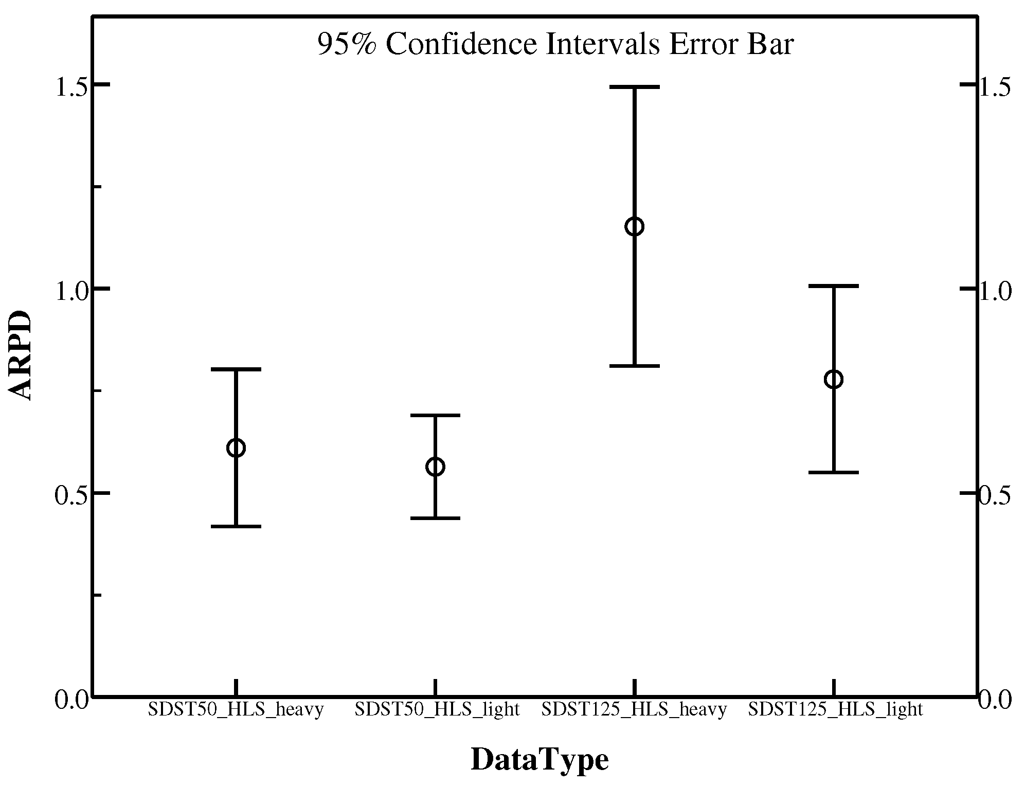
In GlobalSearch, a perturbation has applied to disturb some individuals which trapped in local optima of the current population in terms of balancing the exploration and exploitation. It has an important role in finding individuals with high quality and reducing the further local search. However, there are many kinds of perturbation operators with different effects on the proposed algorithm. Here, two operators consisting of light and heavy perturbation mentioned before are compared by the experiments using instances Ta071–Ta080 in SDST50 and SDST125. In order to compare fairly, it is necessary to make sure the rest frameworks are the same. The effect of the two perturbations details in Table 9 which the better results are marked in bold.
From Table 9, for the instances in SDST50, the heavy perturbation method performs better in Ta072, Ta074, Ta078 and Ta080. In contrast, the light perturbation behaves better in the other seven instances. In terms of the instances in SDST125, the light perturbation also performs better in most of the instances including Ta072, Ta073, Ta074, Ta075, Ta076, Ta077, Ta078 and Ta080. However, the heavy perturbation beats the light one only in instances Ta071 and Ta079. Figure 8 can provide the direct comparison between the two methods. It is proved that the light perturbation exhibits the superior performance in gaining better overall ARPD compared with the heavy perturbation. To conclude, the heavy perturbation is a quite efficient method to help the individuals quit the local optimal condition.
4.6. Effectiveness Evaluation of Different Local Search Operators
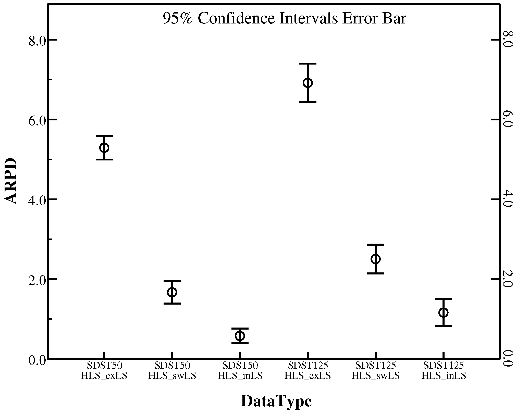
In the beginning search process and the further search of the proposed algorithm, an insertion-based local search local search was executed to find individuals with better fitness in the neighbour search space. Different types of local search can guide the individuals to different directions no matter they are good or bad. In this section, two other local search operators are used to compare with the effective insertion-based local search by instances from Ta071 to Ta080 () in SDST50 and SDST125 running ten times. The compared two operators can be described as follows.
- (1)
- exchange_based local search: For the positions ranging from 1 to of the scheduling permutation, exchange the job in it with the job in the adjacent next position.
- (2)
- swap_based local search: For every position of the scheduling permutation (from 1 to n), swap the job in it with the job in the given position.
It is noted that the other frameworks are the same in this comparison to make the comparison fair. Table 10 demonstrates the details of the three operators. The better results are marked in bold. There are definite differences among these three local search operators. For the standard deviation (SD) of these instances in SDST50 and SDST125, the insertion-based local search has the smallest standard deviation 0.26 and 0.47 respectively among these local search methods. It means that the insertion-based local search is much stabler in getting high-qualified solutions. Furthermore, ARPD that obtained by the insertion-based local search of HLS is much smaller. Hence, it is obvious that the insertion-based local search which can generate high quality solutions performs better than other two methods on all the instances in SDST50 and SDST125. Figure 9 demonstrates that the insertion-based local search in the proposed algorithm can yield better overall mean namely ARPD. In conclusion, the insertion-based local search exhibits its superior performance with high efficiency in the proposed algorithm.
4.7. Comparison Results with Some State-Of-The-Art Approaches
In this subsection, the proposed algorithm with the best algorithm settings yielded from preceding sections is tested with six compared benchmark algorithms containing GA, MA, MA, IG_RS, IG_RS and PACO which can be found in the literature [38] to present a comprehensive performance comparison. Among them IG_RS and MA are integrated IG_RS and MA respectively with an effective local search. To examine the relative ranking of all the algorithms which are dependent on the computation time with the comparative performances, three series of experiments setting the f aforesaid at 30, 60 and 90 are carried out. For each benchmark instance in the following experiments, HLS runs independently ten times and thirty times. HLS(10) denotes the running time of HLS is ten, while HLS(30) represents that HLS is running thirty times. RPD is calculated to compare the performance of different algorithms for each instance. Besides, the standard deviations for each type of instances are calculated to show the robustness of the compared algorithms. The comparative results are shown from Table 11, Table 12, Table 13, Table 14, Table 15 and Table 16 grouped by instances type and size. Because of the limitation of space, only the average RPD of problems in 12 different scales is presented in the sets including SDST10, SDST50, SDST100 and SDST125. It means that ARPD values for each scale with 10 instances, ARPD and SD of all the scales in each type of instance sets are shown in the corresponding tables. The best results of ARPD for the specific algorithm are marked at bold. Besides the negative values represent that the results found by HLS are better than the current best solution provided in http://soa.iti.es/problem-instances. It has to be noted that in the following analyses the ARPDs are achieving by HLS running ten times and the improvement of ARPD means the decrease of that value compared with a certain value because the lower value of ARPD represents the better performance of the algorithm.
From ARPD through Table 11, which the computation time is , the algorithms except for HLS, the best cross ARPD are all gained by IG_RS. It is said that the IG_RS owns the optimal performance in the compared algorithms. In SDST10, HLS can provide slightly better results for instances in the scales from 20 × 5 to 200 × 20 than the algorithm IG_RS. Among them, the maximum improvement compared with IG_RS is 0.41 in the scale of 100 × 20 and the minimum improvement is 0.01 for the scale of 20 × 10. As for the instances in large scale 500 × 20, IG_RS gives a better result of ARPD which is 0.46 than the ARPD of our proposed algorithm 0.72. For the rest algorithms, HLS performs better than all of them in obtaining better ARPD which has the lower value. Overall HLS is better than IG_RS that is the suboptimal algorithm with an ARPD improvement of 0.17. In SDST50, the promotion of ARPD which is developed by HLS has a bit improvement than the type of SDST10. Except for the scale of 500 × 20, HLS presents the best performance on each scale among all the algorithms. But in terms of ARPD in the scale 500 × 20, HLS is just next to IG_RS and is superior to the rest algorithms owing the second-best performance. The least improvement of ARPD is 0.04 and the most improvement is 0.99 compared with the suboptimal RPD obtained by IG_RS. To the overall ARPD, HLS beats all the other algorithms on average with the value of 0.45, better than ARPD 1.00 of IG_RS. The ranking order of the algorithms as the best performing to the worst performing are HLS, IG_RS, MA, MA, IG_RS, PACO and GA.
From Table 12, for the large sets SDST100 and SDST125, HLS can generate better results compared to the small sets including SDST10 and SDST50. For SDST100, the least difference which is better than IG_RS is 0.19 which is the difference between 0.27 and 0.08 in the scale of 20 × 20. The above data records the most difference is 1.30. The values of ARPD in each scale of instances gaining by HLS are all the best with the exception of the scale 500 × 20. Considering the cross average in this table, the ranking of HLS is best. For SDST125, the least and the most difference which are improved compared with IG_RS are 0.19 and 1.58 respectively. Seen from the overall ARPD, there is an ARPD 0.62 developed by HLS better than the other algorithms and it has the value of 0.82 in terms of the improvement compared with the suboptimal ARPD in the algorithm IG_RS. It is noted that it has a much higher average percentage promotion than other five algorithms. It also implies that HLS can provide better performance with the increase of ratio between the setup times and the processing times.
From Table 13 and Table 14, which are ARPD results of all the types in all the instances when we set the computation time as , the same pattern are obtained in the four data sets. With the exception of the instances in 500 × 20, all other ARPD are improved rather better gradually with the increase of the setup times in the range of SDST10, SDST50, SDST100 and SDST125. It is clear that HLS exceeds all other algorithms because of its good performance on the least overall ARPD.
It is the same as Table 15 and Table 16 when the computation time is . For SDST50, except for the scale of 500 × 20, ARPD of each algorithm in each scale decreases as the order of GA, PACO, IG_RS, MA, MA, IG_RS, HLS, which shows the best performance of HLS among all the compared algorithms. For SDST100 and SDST125, it is shown the same pattern. However, the tendency of increasing softens in SDST10 with the exceptions of ARPD in the scale of 20 × 10 and 500 × 20. For brevity, the remaining analyses of the minimum and maximum of ARPD between the relatively good two algorithms which are HLS and IG_RS in each scale are omitted. But the trend of performance for each algorithm is the same as the previous tables has shown. As we can see from the overall ARPD, it is evident that there is the least ARPD in HLS which surpasses by other algorithms attributed to the high effectiveness of each component in HLS. Furthermore, via the standard deviations from Table 11, Table 12, Table 13, Table 14, Table 15 and Table 16 of each compared algorithm, it is demonstrated that the high stability of HLS in gaining good solutions.
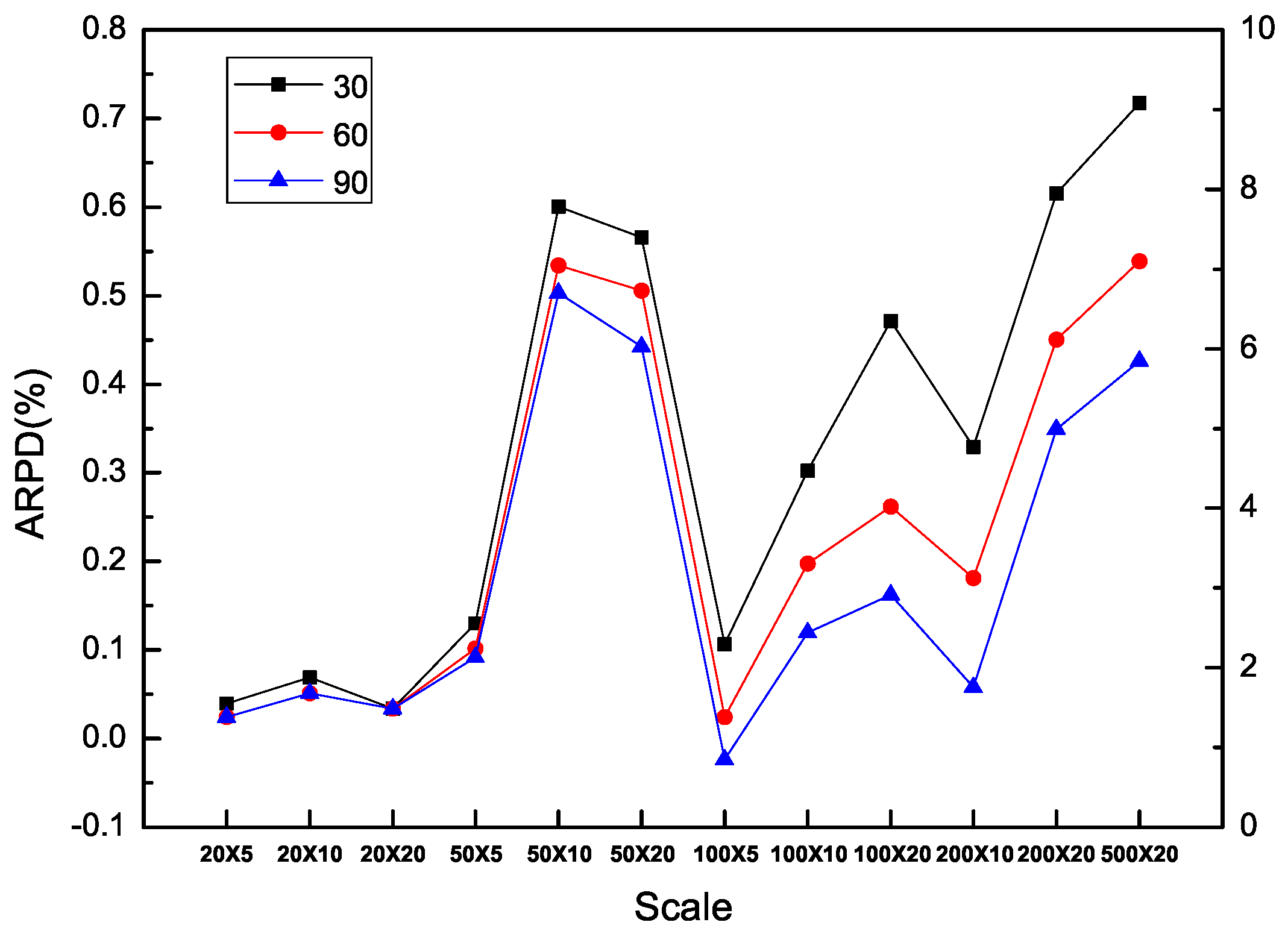
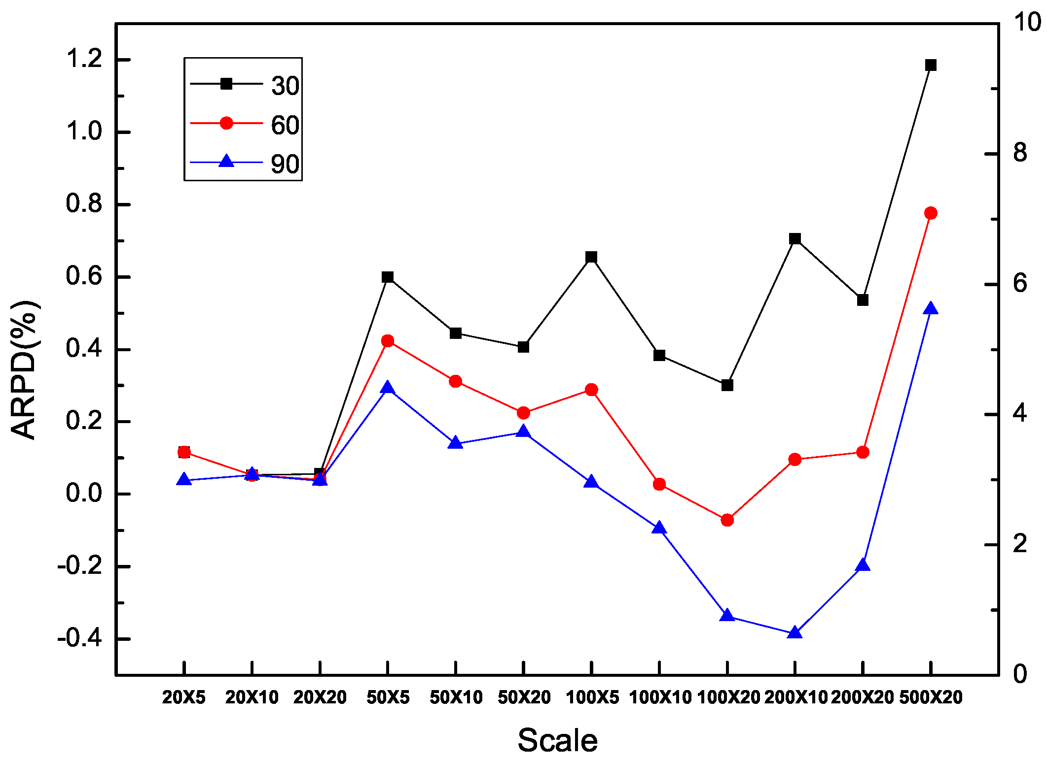
In addition, it is obvious that each algorithm is benefited from additional computation time in all the types of instances including SDST10, SDST50, SDST100 and SDST125. Figure 10, Figure 11, Figure 12 and Figure 13 are used to prove the importance of the computation time in different scales of instances by ARPD evaluated with HLS running ten times. The trajectory of each curse in the figure overall declines and becomes closer to the X axis along with the increase of f which represents the better cross ARPD. Besides, it is also found that the average RPD shows an increasing trend because the increase of the instance size in the number of machines classified by the number of jobs including 20, 50, 100, 200 and 500. Via the above figures, what can be summarized is that the value of the cross ARPD is decreasing and becomes better clearly with the increase of f regardless of the instance type and instance size.
Besides, the interactions between the ratio of the setup times in the processing times and the scales have to be studied to verify the effectiveness of HLS. It is shown in Figure 14, Figure 15 and Figure 16 to present the different types of instances segregated by f = 30, 60 and 90 for HLS running ten times respectively. As a matter of fact, the average RPD has reduced rather more acutely with a larger difference in each algorithm for the large type of SDST100 and SDST125 compared with the type sets of SDST10 and SDST50. Moreover, the trend of each curve in Figure 15 and Figure 16 demonstrates the performance ranking of these compared algorithms are as the ascendent order of GA, PACO, IG_RS, MA, MA, IG_RS, HLS visually. However, Figure 14 has presented the descendent performance order of algorithms is HLS, IG_RS, MA, IG_RS, MA, PACO and GA. It is summarized that HLS gives higher priority to the increase of the computation time and the increase ratio between the setup time and the processing time.
The next tables from Table 17, Table 18, Table 19, Table 20, Table 21, Table 22 and Table 23 present the newbounds of makespan discovered by HLS running ten times and the aforementioned best-known bounds grouped by different scales in different types of instances. The differences between the two values are presented in the tables which shows the high effectiveness in getting high-qualified solutions of HLS. Besides, they become larger as the increase of the ratio of the setup times in the processing times and the scales of instances. By the same pattern, the number of newbounds has raised progressively. For an example, in the scale 50 × 5, the difference in Ta039 of SDST10 is −2, but for Ta038 of SDST100, the difference is −27. Table 18 provides the newbounds, the best-known bounds and the differences between them for the instances in the scale 50 × 10. Hence, it is evident that the differences are bigger in SDST50 and SDST100 overall which mean that HLS is much more effective. The tables are shown that HLS is statistically superior to other well-performing algorithms. For the illustration purpose, what follows it is Table 24 that shows some permutations of jobs chosen from the scale 50 × 5 in the instances of SDST10 and SDST100 because of space limitations. The permutation sequence begins from 0 and ends in 49 in each instance which is the best solution with the newbound of makespan developed by HLS.
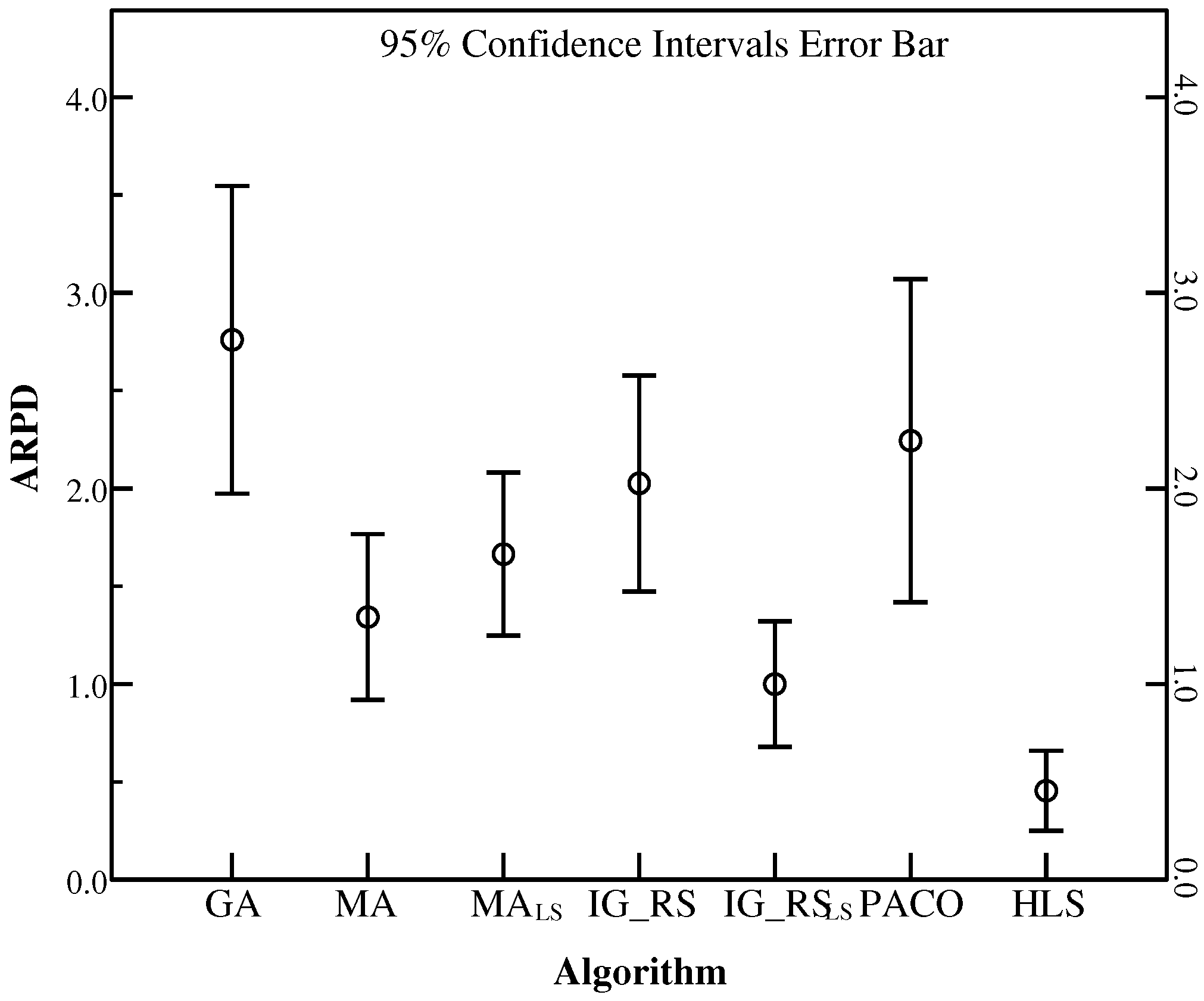
To illustrate the robustness of HLS, the instances in the set SDST50 are chosen to be the base examples. Besides, Figure 17, Figure 18 and Figure 19 use ARPD in confidence intervals at the 95% confidence level taking the CPU time of , and respectively to analyse the robustness. The ARPDs here are developed by HLS running ten times. The length of the error bar represents the stability degree of each algorithm. It means if the length of the bar for one algorithm is short, then the algorithm gives the better robustness. It is clearly shown that HLS has the strongest robustness with the shortest interval among all the compared algorithms no matter how long the CPU time is. The robustness order of other algorithms are PACO, GA, IG_RS, MA, MA, IG_RS from worst to best as the above figures have provided. Moreover, the above figures have presented the best effectiveness of HLS with a smallest value of the average RPD. As a result, the average RPD also shows that the effectiveness ranking of other algorithms is GA, PACO, IG_RS, MA, MA, IG_RS from the last rank to the first rank. Although PACO has the better effectiveness which has a lower ARPD compared with GA, in terms of robustness GA is stabler than PACO. Through synthetical consideration of the effectiveness and the robustness for each algorithm, HLS is resulted to the best algorithm in all the compared algorithms.
As we can see from the above tables and figures, it can be concluded that it is GA, PACO, IG_RS, MA, MA, IG_RS, HLS from the worst to the best performance for the comprehensive consideration particularly because ARPD of all the 480 instances is decreasing in line. Although in the instances of the scale 500 × 20, IG_RS can provide a better ARPD, HLS can present a better overall ARPD regardless of instance type. Besides, HLS performs much better as the increase ratio of the setup times in the processing times. Based on the above results, it can be said that HLS performs better than other six algorithms. It is verified that HLS is an effective and robust algorithm for solving the flowshop scheduling problem with sequence dependent setup times.
4.8. Comparison Results with Some Recent Algorithms
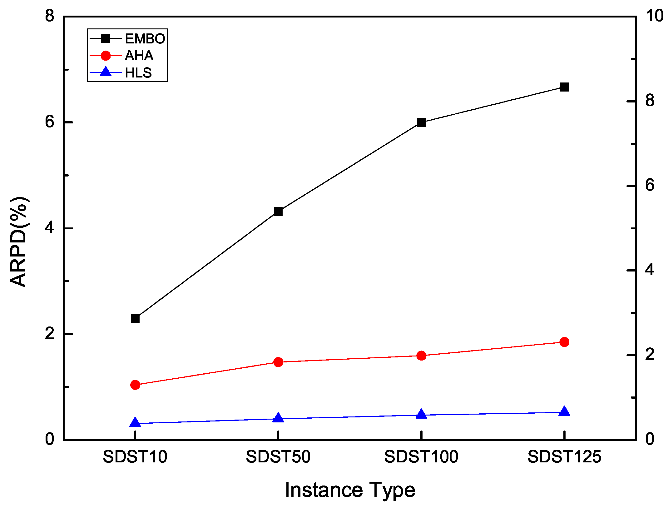
In order to further illustrate the effectiveness of the proposed algorithm, we reconstruct an experiment to compare with two recent algorithms, namely the adaptive hybrid algorithm (AHA) [39], and the enhanced migrating birds optimization (EMBO) [40] for FSSP-SDST with the makespan criterion.
In AHA, each job is assigned an inheriting factor. For dynamically updating the factor, a novel operator is constructed. Therefore, both good and bad genes can be explored. A new crossover operator is proposed by inheriting good genes to the offspring and destroying the bad genes with a high probability. Hence, the offspring is integrated with more and more good genes generation after some generations. It helps to improve the effectiveness of AHA in obtaining high-qualified solutions. The algorithm AHA is chosen to compare with HLS. Besides, for the migrating birds optimization (MBO) [41], it is a metaheuristic inspired from the flight of migrating birds. To save the energy, the known V-flight shape3 is developed. Thereafter, a basic migrating birds optimization (BMBO) [23] is proposed to solve FSSP-SDST with the makespan criterion. In terms of EMBO, since the performance of BMBO keeps decreasing with the increase in the size of instances, EMBO is based on the BMBO with an or-opt neighbourhood which was designed for the travelling salesman problem (TSP) first and the well-known heuristics to generate its leader bird. The or-opt neighbourhood operator is moving a block of one, two, three jobs or four jobs and inserting it elsewhere in the sequence.
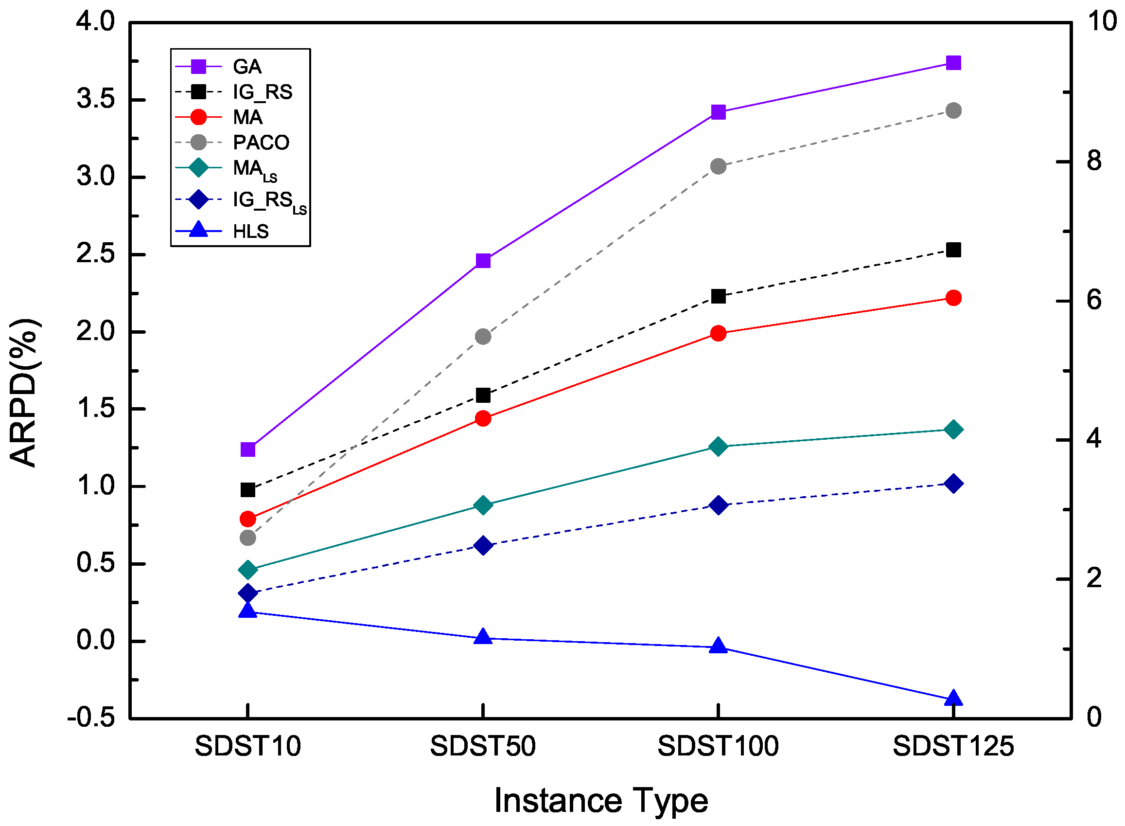
HLS runs 30 times to compare with the above algorithms. The RPD results for each scale data in SDST10, SDST50, SDST100, SDST125 of each compared algorithm is presented in Table 25. The relatively good results are marked in bold. From Table 25, it is seen that HLS is more suitable than the other compared algorithms for achieving good results. In detail, HLS has the best values of ARPD 0.31 and 0.40 in SDST10 and SDST50 respectively among the ARPDs gaining by the compared algorithms. For SDST100 and SDST125, the values of the overall ARPD are 0.47 and 0.52 which are clearly better than the other ARPD values of EMBO and AHA. In addition, Figure 20 is presented to show the good effectiveness of HLS in obtaining high-qualified results intuitively.
In conclusion, HLS is very competitive to the good performing algorithms for solving FSSP-SDST with makespan criterion.
5. Conclusions and Future Work
In this paper, the flowshop scheduling problem with sequence dependent setup times is addressed with minimizing the makespan. A hybrid local search algorithm based on novel local search methods is presented to deal with this problem. First, to initialize the population, we apply an effective NEH based problem-specific method to the initialize the population. Second, the global search embedded with a light perturbation is used to generate the better population. Then, to find good individuals in the current population, the insertion-based local search is adopted. Next, a further local search is applied to individuals which are trapped into local optima. Last, a heavy perturbation is used to explore better neighbours in the new research regions.
In order to demonstrate the performance of the proposed algorithm, extensive experiments are conducted on all the 120 instances of four different scales. It is obviously shown in the compared experiments that HLS gives better results than other six state-of-the-art algorithms, including GA, MA, MA, IG_RS, IG_RS and PACO. The experimental results confirm that it is appropriate in using the combination of local search and perturbation methods in HLS.
In the future, the proposed HLS algorithm is expected to be used to solve other combinational problems such as no-wait flowshop scheduling problems (NWFSSP), hybrid flowshop scheduling problems (HFSSP), blocking flowshop scheduling problems (BFSSP) under makespan criterion. Different values of parameters for HLS can be experimented comprehensively to enhance the solution quality. In addition, different neighbourhood structures can be developed for improving the effectiveness of HLS. Meanwhile, the interactions between the exploitation and the exploration strategies should be investigated in depth. In other words, other techniques on different ways of local search and perturbation which is more suitable for FSSP-SDST can be studied to guide the search to other extensive spaces and enhance the performance of HLS. Moreover, it helps to construct other metaheuristics with some effective ingredients adding to the basic HLS. For example, the restart strategy that a new population is generated randomly with the current best individual not improving after a given number of iterations and the elite strategy that keeps some elite individuals in current population for a number of iterations.
Furthermore, we can integrate HLS with other heuristics, such as the variable neighbourhood search and the tabu search. This would be more effective to keep balance between the intensification and the diversification and improve the quality of solutions.
Acknowledgments
The authors would like to thank all anonymous reviewers for their constructive comments, which have helped improve the study in numerous ways. This research is supported by the National Natural Science Foundation of China under Grant No. 61603087 and also funded by the Natural Science Foundation of Jilin Province under Grant No. 20160101253JC. Meanwhile, this research is also supported by the Fundamental Research Funds for the Central Universities No. 2412017FZ026.
Author Contributions
Yunhe Wang operated the experiments and drafted the manuscript. Xiangtao Li designed the research and Zhiqiang Ma checked the manuscript.
Conflicts of Interest
The authors declare no conflict of interest.
Abbreviations
The following abbreviations are used in this manuscript:
| FSSP-SDST | The flowshop scheduling problem with sequence dependent setup times |
| HLS | Hybrid local search algorithm |
| NEHBPS | Nawaz-Enscore-Hoam based problem-specific method |
| RPD | Relatively percentage deviation |
References
- Johnson, S.M. Optimal two- and three-stage production schedules with setup times included. Nav. Res. Logist. Q. 1954, 1, 61–68. [Google Scholar] [CrossRef]
- Cheng, T.C.E.; Gupta, J.N.D.; Wang, G. A review of flowshop scheduling reasearch with setup times. Prod. Oper. Manag. 2000, 9, 262–282. [Google Scholar] [CrossRef]
- Vanchipura, R.; Sridharan, R. Development and analysis of constructive heuristic algorithms for flow shop scheduling problems with sequence-dependent setup times. Int. J. Adv. Manuf. Technol. 2013, 67, 1337–1353. [Google Scholar] [CrossRef]
- Kheirkhah, A.; Navidi, H.; Bidgoli, M.M. Dynamic facility layout problem: A new bilevel formulation and some metaheuristic solution methods. IEEE Trans. Eng. Manag. 2015, 62, 396–410. [Google Scholar] [CrossRef]
- Balouka, N.; Cohen, I.; Shtub, A. Extending the Multimode Resource-Constrained Project Scheduling Problem by Including Value Considerations. IEEE Trans. Eng. Manag. 2016, 63, 4–15. [Google Scholar] [CrossRef]
- Li, S.; Wang, N.; Jia, T.; He, Z.; Liang, H. Multiobjective Optimization for Multiperiod Reverse Logistics Network Design. IEEE Trans. Eng. Manag. 2016, 63, 223–236. [Google Scholar] [CrossRef]
- Kheirkhah, A.; Navidi, H.; Bidgoli, M.M. An Improved Benders Decomposition Algorithm for an Arc Interdiction Vehicle Routing Problem. IEEE Trans. Eng. Manag. 2016, 63, 259–273. [Google Scholar] [CrossRef]
- Rios-Mercado, R.Z.; Bard, J.F. The flow shop scheduling polyhedron with setup times. J. Comb. Optim. 2003, 7, 291–318. [Google Scholar] [CrossRef]
- Nishi, T.; Hiranaka, Y. Lagrangian relaxation and cut generation for sequence-dependent setup time flowshop scheduling problems to minimise the total weighted tardiness. Int. J. Prod. Res. 2013, 51, 4778–4796. [Google Scholar] [CrossRef]
- Christian, B.; Andrea, R.; Michael, S. Hybrid Metaheuristics: An Emerging Approach to Optimization; Studies in Computational Intelligence; Springer: Berlin, Germany, 2008; Volume 114. [Google Scholar]
- Raidl, G.R.; Puchinger, J. Combining (Integer) Linear Programming Techniques and Metaheuristics for Combinatorial Optimization. Hybrid Metaheuristics 2008, 114, 31–62. [Google Scholar]
- Blum, C.; Cotta, C.; Fernandez, A.; Sampels, M. Hybridizations of metaheuristics with branch & bound derivates. Hybrid Metaheuristics 2008, 114, 85–116. [Google Scholar]
- D’Andreagiovanni, F.; Nardin, A. Towards the fast and robust optimal design of wireless body area networks. Appl. Soft Comput. 2015, 37, 971–982. [Google Scholar] [CrossRef]
- D’Andreagiovanni, F.; Krolikowski, J.; Pulaj, J. A fast hybrid primal heuristic for multiband robust capacitated network design with multiple time periods. Appl. Soft Comput. 2015, 26, 497–507. [Google Scholar] [CrossRef]
- Gambardella, L.M.; Montemanni, R.; Weyland, D. Coupling ant colony systems with strong local searches. Eur. J. Oper. Res. 2012, 220, 831–843. [Google Scholar] [CrossRef]
- Nawaz, M.; Enscore, E.E.; Ham, I. A heuristic algorithm for the m-machine, n-job flow-shop sequencing problem. Omega 1983, 11, 91–95. [Google Scholar] [CrossRef]
- Rios-Mercado, R.Z.; Bard, J.F. Heuristics for the flow line problem with setup costs. Eur. J. Oper. Res. 1998, 110, 76–98. [Google Scholar] [CrossRef]
- Ruiz, R.; Maroto, C.; Alcaraz, J. Solving the flowshop scheduling problem with sequence dependent setup times using advanced metaheuristics. Eur. J. Oper. Res. 2005, 165, 34–54. [Google Scholar] [CrossRef]
- Rios-Mercado, R.Z.; Bard, J.F. An Enhanced TSP-Based Heuristic for Makespan Minimization in a Flow Shop with Setup Times. J. Heuristics 1999, 5, 53–70. [Google Scholar] [CrossRef]
- Rajendran, C.; Ziegler, H. Ant-colony algorithms for permutation flowshop scheduling to minimize makespan/total flowtime of jobs. Eur. J. Oper. Res. 2004, 155, 426–438. [Google Scholar] [CrossRef]
- Gajpal, Y.; Rajendran, C.; Ziegler, H. An ant colony algorithm for scheduling in flowshops with sequence-dependent setup times of jobs. Int. J. Adv. Manuf. Technol. 2006, 30, 416–424. [Google Scholar] [CrossRef]
- Tseng, F.T.; Gupta, J.N.D.; Stafford, E.F. A penalty-based heuristic algorithm for the permutation flowshop scheduling problem with sequence-dependent set-up times. J. Oper. Res. Soc. 2006, 57, 541–551. [Google Scholar] [CrossRef]
- Benkalai, I.; Rebaine, D.; Gagne, C.; Baptiste, P. The migrating birds optimization metaheuristic for the permutation flow shop with sequence dependent setup times. IFAC PapersOnLine 2016, 49, 408–413. [Google Scholar] [CrossRef]
- Simons, J.V. Heuristics in flow shop scheduling with sequence dependent setup times. Omega 1992, 20, 215–225. [Google Scholar] [CrossRef]
- Jacobs, L.W.; Brusco, M.J. Note: A local-search heuristic for large set-covering problems. Nav. Res. Logist. 1995, 42, 1129–1140. [Google Scholar] [CrossRef]
- Ruizab, R. A simple and effective iterated greedy algorithm for the permutation flowshop scheduling problem. Eur. J. Oper. Res. 2007, 177, 2033–2049. [Google Scholar]
- Rajendran, C.; Ziegler, H. A heuristic for scheduling to minimize the sum of weighted flowtime of jobs in a flowshop with sequence-dependent setup times of jobs. Comput. Ind. Eng. 1997, 33, 281–284. [Google Scholar] [CrossRef]
- Wang, Y.; Dong, X.; Chen, P.; Lin, Y. Iterated Local Search Algorithms for the Sequence-Dependent Setup Times Flow Shop Scheduling Problem Minimizing Makespan. In Foundations of Intelligent Systems; Springer: Berlin/Heidelberg, Germany, 2014; pp. 329–338. [Google Scholar]
- Li, X.; Yin, M. An opposition-based differential evolution algorithm for permutation flow shop scheduling based on diversity measure. Adv. Eng. Softw. 2013, 55, 10–31. [Google Scholar] [CrossRef]
- Li, X.; Yin, M. A hybrid cuckoo search via Levy flights for the permutation flow shop scheduling problem. Int. J. Prod. Res. 2013, 51, 4732–4754. [Google Scholar] [CrossRef]
- Li, X.; Yin, M. A discrete artificial bee colony algorithm with composite mutation strategies for permutation flow shop scheduling problem. Sci. Iran. 2012, 19, 1921–1935. [Google Scholar] [CrossRef]
- Wang, L.; Fang, C. A hybrid estimation of distribution algorithm for solving the resource-constrained project scheduling problem. Expert Syst. Appl. 2012, 39, 2451–2460. [Google Scholar] [CrossRef]
- Fang, C.; Wang, L. An effective shuffled frog-leaping algorithm for resource-constrained project scheduling problem. Inf. Sci. 2011, 181, 4804–4822. [Google Scholar] [CrossRef]
- Pan, Q.K.; Wang, L. Effective heuristics for the blocking flowshop scheduling problem with makespan minimization. Omega 2012, 40, 218–229. [Google Scholar] [CrossRef]
- Li, X.; Wang, Q.; Wu, C. Efficient composite heuristics for total flowtime minimization in permutation flow shops. Omega 2009, 37, 155–164. [Google Scholar] [CrossRef]
- Li, X.; Ma, S. Multi-Objective Memetic Search Algorithm for Multi-Objective Permutation Flow Shop Scheduling Problem. IEEE Access 2017, 4, 2154–2165. [Google Scholar] [CrossRef]
- Li, X.; Li, M. Multiobjective Local Search Algorithm-Based Decomposition for Multiobjective Permutation Flow Shop Scheduling Problem. IEEE Trans. Eng. Manag. 2015, 62, 544–557. [Google Scholar] [CrossRef]
- Ruizab, R. An Iterated Greedy heuristic for the sequence dependent setup times flowshop problem with makespan and weighted tardiness objectives. Eur. J. Oper. Res. 2008, 187, 1143–1159. [Google Scholar]
- Li, X.; Zhang, Y. Adaptive hybrid algorithms for the sequence-dependent setup time permutation flow shop scheduling problem. IEEE Trans. Autom. Sci. Eng. 2012, 9, 578–595. [Google Scholar] [CrossRef]
- Benkalai, I.; Rebaine, D.; Gagne, C.; Baptiste, P. Improving the migrating birds optimization metaheuristic for the permutation flow shop with sequence-dependent set-up times. Int. J. Prod. Res. 2017, 1–13. [Google Scholar] [CrossRef]
- Duman, E.; Uysal, M.; Alkaya, A.F. Migrating Birds Optimization: A new metaheuristic approach and its performance on quadratic assignment problem. Inf. Sci. 2012, 217, 65–77. [Google Scholar] [CrossRef]
Figure 1.
Gratt chart for -- to the example problem.
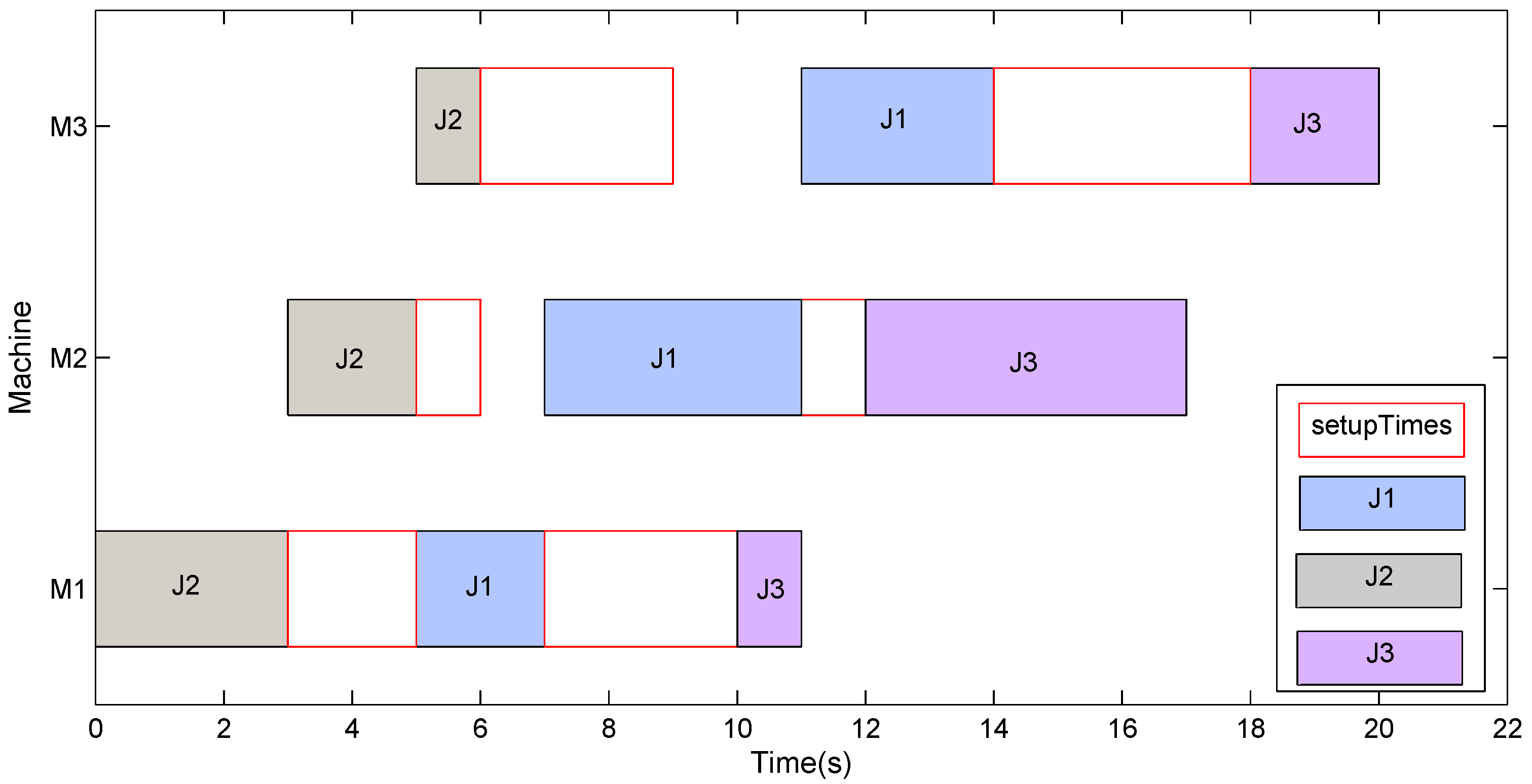
Figure 2.
ARPD plot for Ta071–Ta080 with different numbers of N.
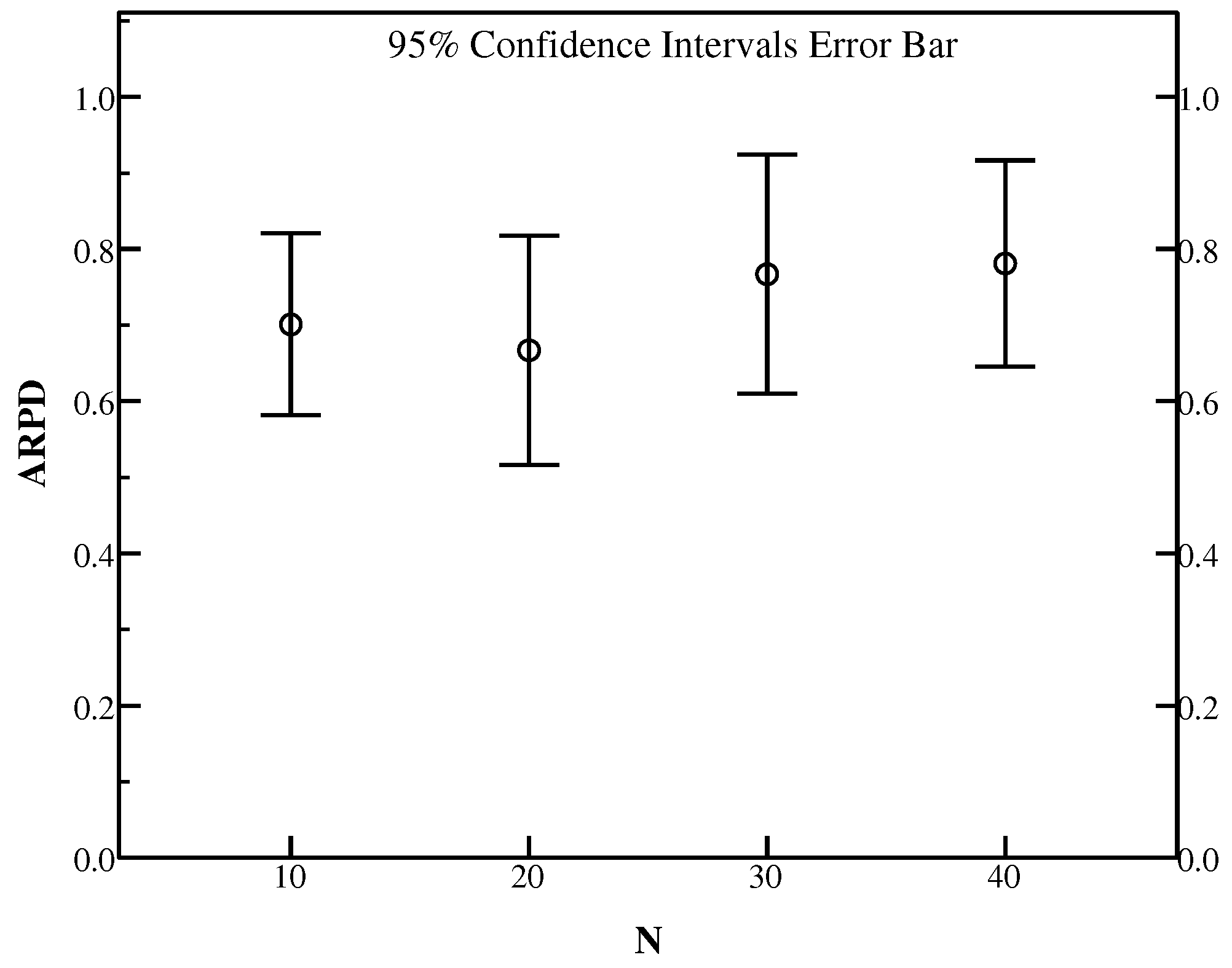
Figure 3.
ARPD plot for Ta071–Ta080 with different numbers of GSNum.

Figure 4.
ARPD plot for Ta071–Ta080 with different numbers of .
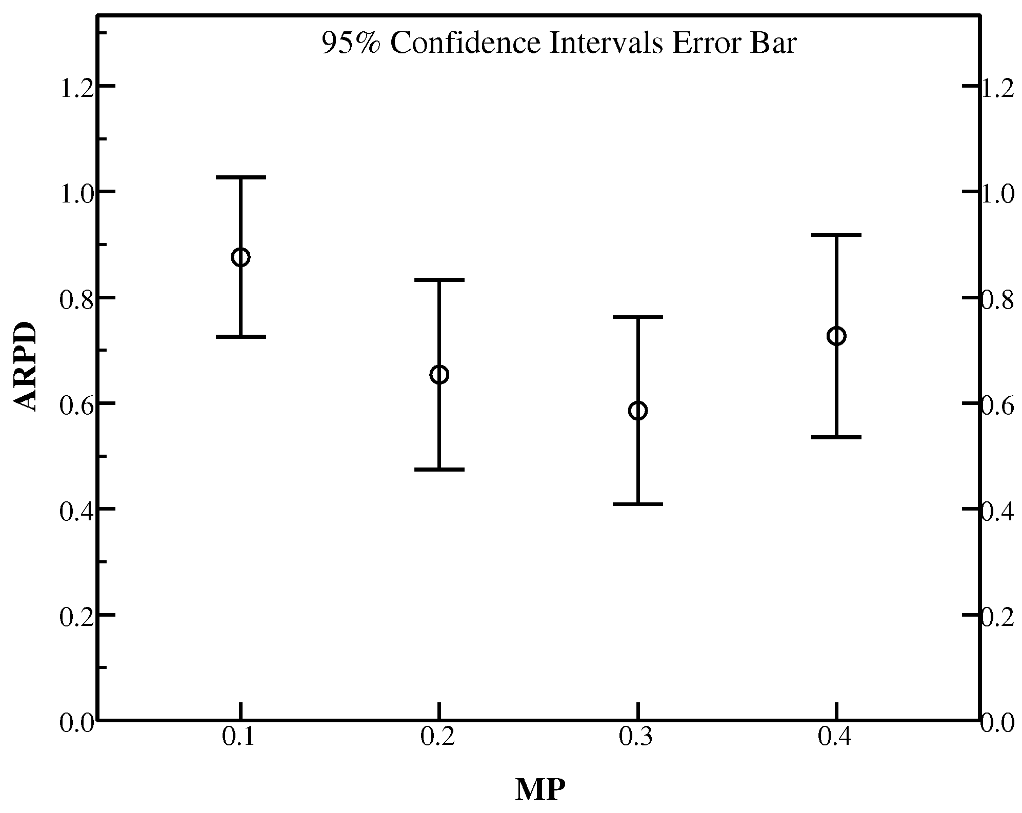
Figure 5.
ARPD plot for Ta071–Ta080 with different numbers of UpdateNum.
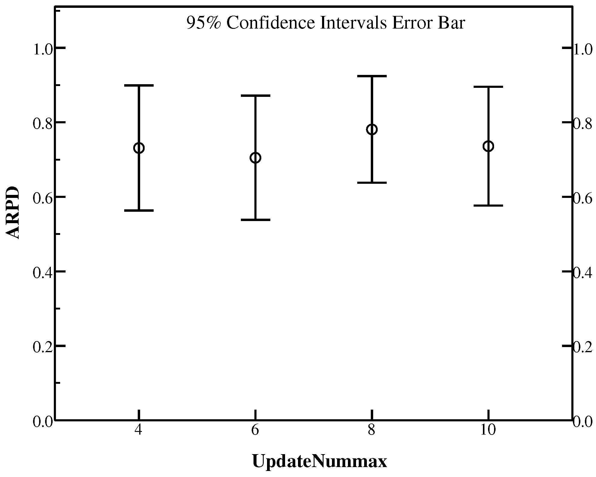
Figure 6.
ARPD plot for Ta071–Ta080 with different numbers of FSNum.

Figure 7.
ARPD plot for SDST50 and SDST125 with or without NEHBPS.

Figure 8.
ARPD plot for SDST50 and SDST125 with different types of local search.

Figure 9.
ARPD plot for SDST50 and SDST125 with different types of local search.

Figure 10.
ARPD plot for SDST10 with the different values of f.

Figure 11.
ARPD plot for SDST50 with the different values of f.

Figure 12.
ARPD plot for SDST100 with the different values of f.
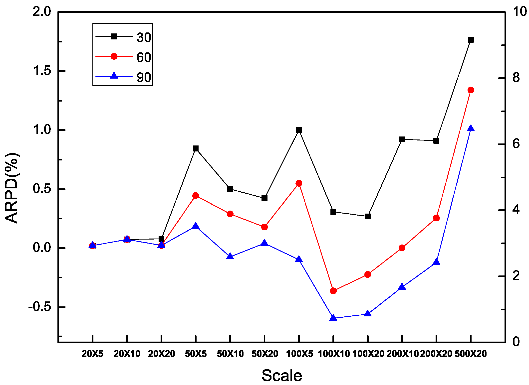
Figure 13.
ARPD plot for SDST125 with the different values of f.
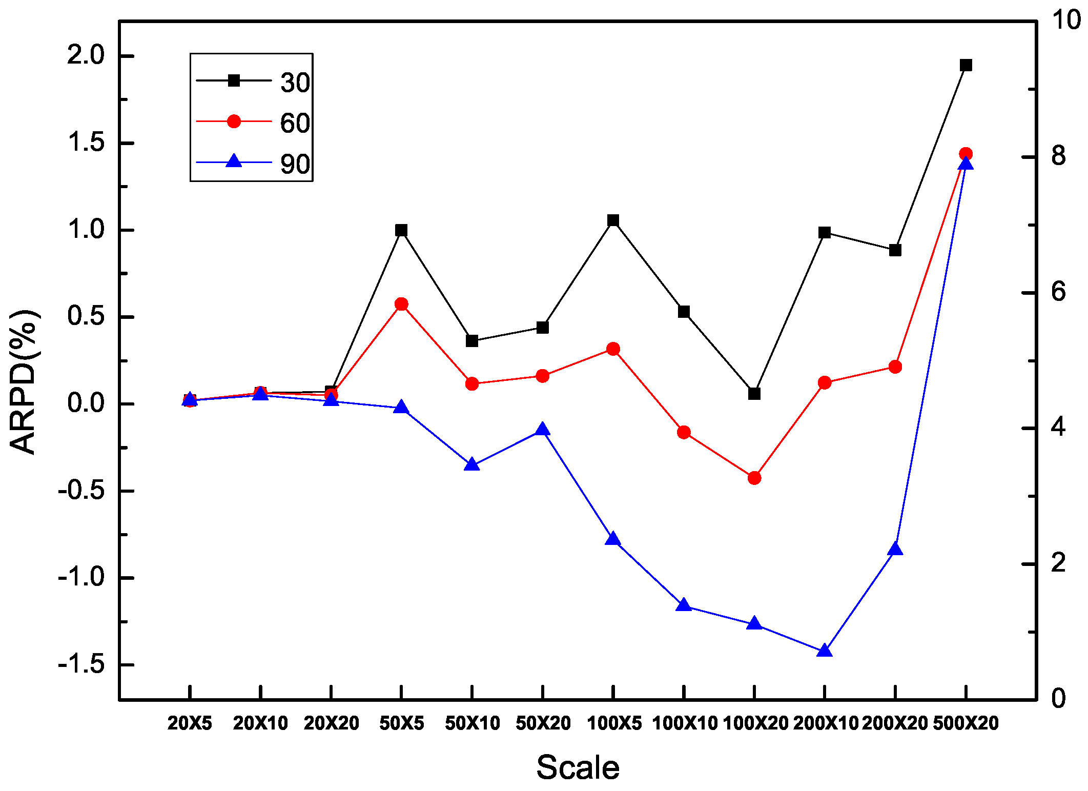
Figure 14.
ARPD comparison of different methods on different types of instances (f = 30).
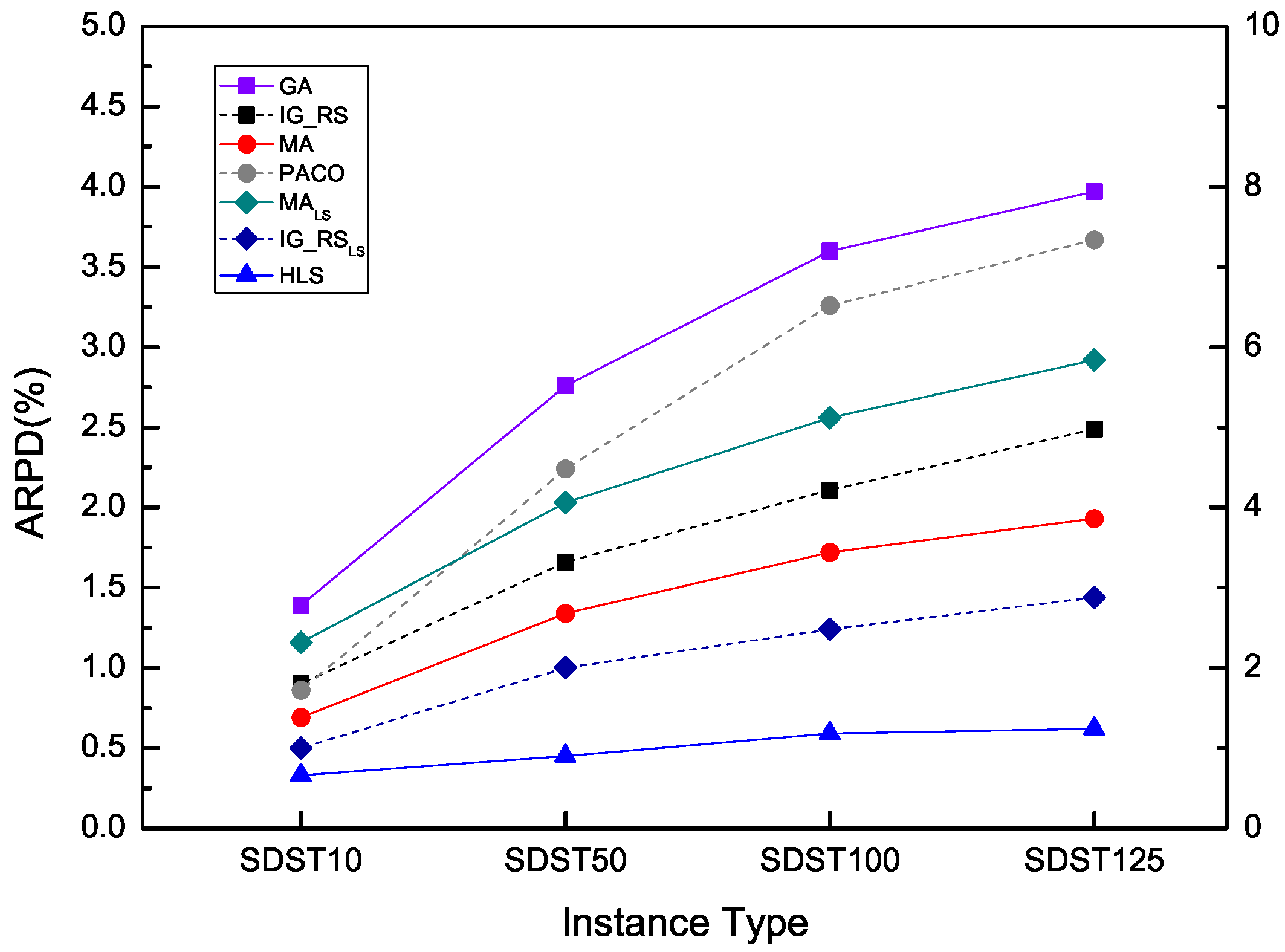
Figure 15.
ARPD comparison of different methods on different types of instances (f = 60).
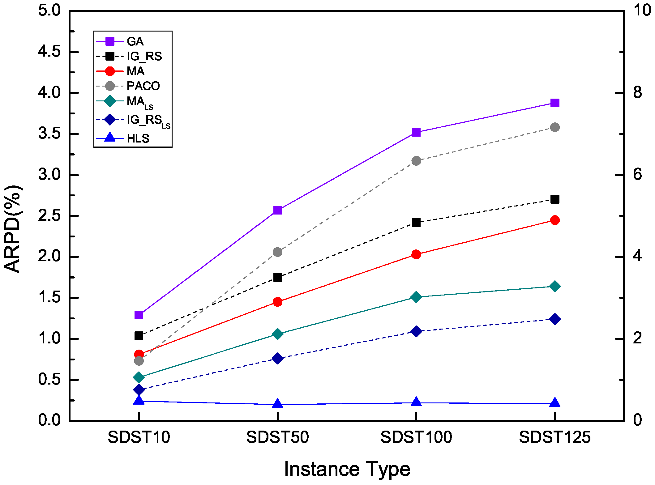
Figure 16.
ARPD comparison of different methods on different types of instances (f = 90).

Figure 17.
ARPD in 95% CI for each algorithm in SDST50 (f = 30).

Figure 18.
ARPD in 95% CI for each algorithm in SDST50 (f = 60).
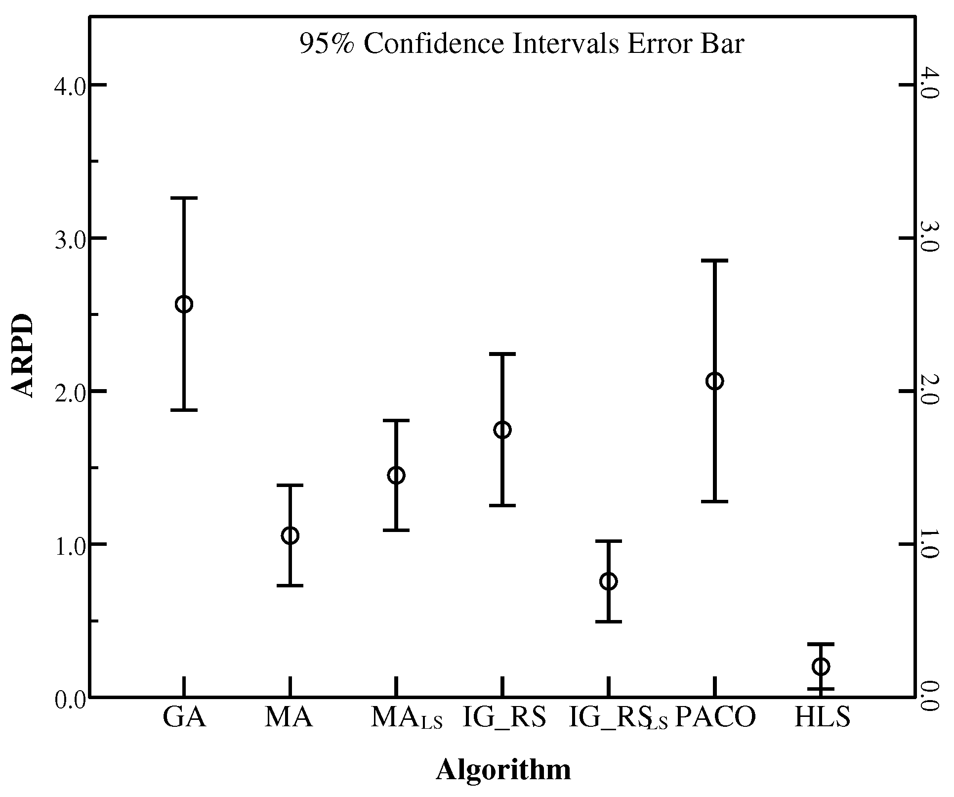
Figure 19.
ARPD in 95% CI for each algorithm in SDST50 (f = 90).
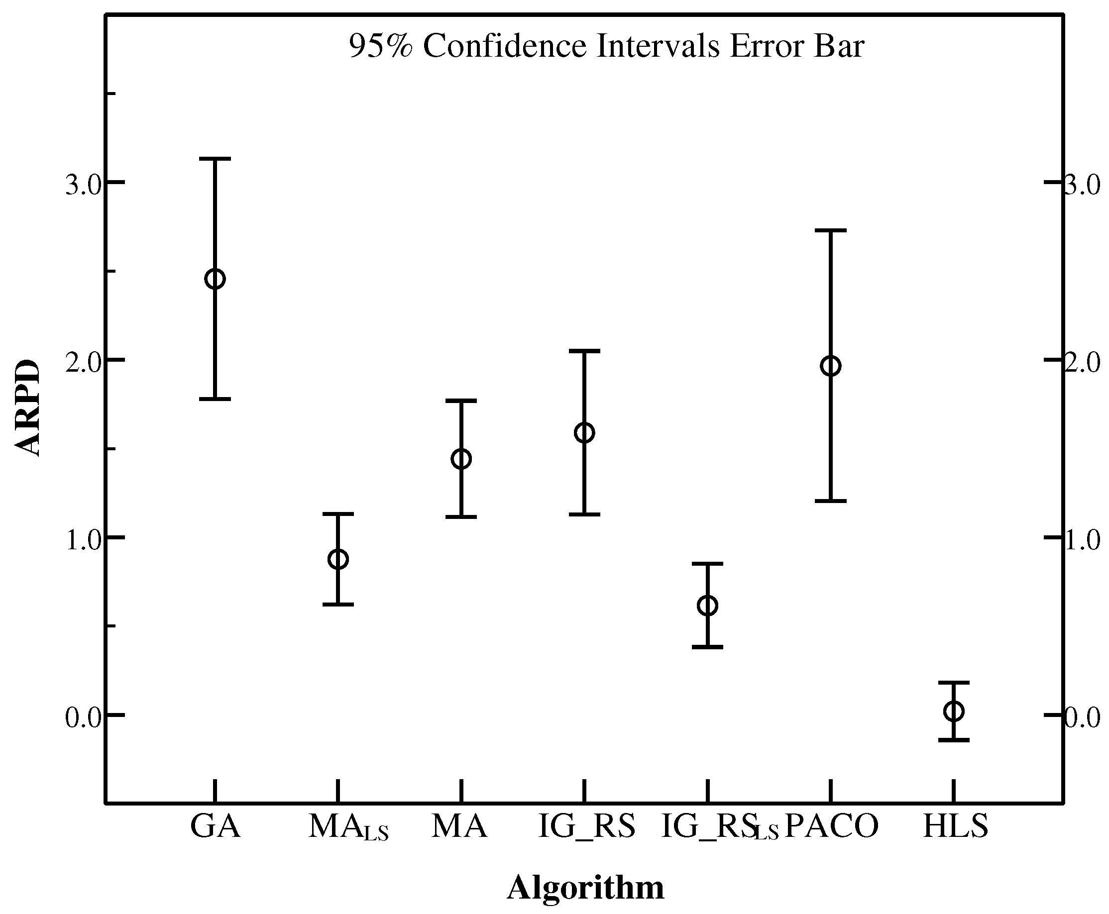
Figure 20.
ARPD comparison for methods on different types of instances.

Table 1.
Processing times of jobs on each machine.
| J1 | J2 | J3 | |
|---|---|---|---|
| M1 | 2 | 3 | 1 |
| M2 | 4 | 2 | 5 |
| M3 | 3 | 1 | 2 |
Table 2.
Sequence dependent setup times of jobs on each machine.
| M1 | M2 | M3 | |||||||||
|---|---|---|---|---|---|---|---|---|---|---|---|
| J1 | J2 | J3 | J1 | J2 | J3 | J1 | J2 | J3 | |||
| J1 | – | 2 | 3 | J1 | – | 3 | 1 | J1 | – | 2 | 4 |
| J2 | 2 | – | 4 | J2 | 1 | – | 3 | J2 | 3 | – | 8 |
| J3 | 3 | 4 | – | J3 | 3 | 2 | – | J3 | 6 | 7 | – |
Table 3.
The RPD of different numbers of N. The bold numbers are the relatively good ARPD results.
| DataNo. | 10 | 20 | 30 | 40 |
|---|---|---|---|---|
| Ta071 | 0.72 | 0.47 | 0.54 | 0.50 |
| Ta072 | 0.80 | 0.81 | 0.94 | 1.17 |
| Ta073 | 0.65 | 0.58 | 0.59 | 0.56 |
| Ta074 | 0.62 | 0.68 | 0.58 | 0.89 |
| Ta075 | 0.70 | 0.46 | 0.77 | 0.76 |
| Ta076 | 0.67 | 1.11 | 1.13 | 0.78 |
| Ta077 | 0.86 | 0.65 | 0.63 | 0.66 |
| Ta078 | 0.41 | 0.41 | 0.88 | 0.80 |
| Ta079 | 0.56 | 0.67 | 0.56 | 0.78 |
| Ta080 | 1.02 | 0.83 | 1.05 | 0.91 |
| Average | 0.70 | 0.67 | 0.77 | 0.78 |
Table 4.
The RPD of different numbers of GSNum. The bold numbers are the relatively good ARPD results.
Table 4.
The RPD of different numbers of GSNum. The bold numbers are the relatively good ARPD results.
| DataNo. | 3 | 4 | 5 | 6 |
|---|---|---|---|---|
| Ta071 | 0.42 | 0.55 | 0.62 | 0.60 |
| Ta072 | 1.22 | 0.91 | 0.94 | 0.90 |
| Ta073 | 0.76 | 0.73 | 0.59 | 0.65 |
| Ta074 | 1.10 | 0.65 | 0.23 | 0.83 |
| Ta075 | 0.86 | 0.22 | 0.77 | 0.62 |
| Ta076 | 0.92 | 0.62 | 1.05 | 0.86 |
| Ta077 | 0.87 | 0.69 | 0.63 | 0.91 |
| Ta078 | 0.82 | 0.29 | 0.40 | 0.55 |
| Ta079 | 0.93 | 0.54 | 0.55 | 0.74 |
| Ta080 | 1.05 | 0.54 | 1.05 | 0.90 |
| Average | 0.89 | 0.57 | 0.68 | 0.76 |
Table 5.
The RPD of different numbers of . The bold numbers are the relatively good ARPD results.
| DataNo. | 0.1 | 0.2 | 0.3 | 0.4 |
|---|---|---|---|---|
| Ta071 | 0.77 | 0.46 | 0.63 | 0.85 |
| Ta072 | 0.94 | 0.90 | 0.55 | 1.02 |
| Ta073 | 0.63 | 0.62 | 0.58 | 0.81 |
| Ta074 | 0.94 | 0.46 | 0.57 | 0.56 |
| Ta075 | 0.51 | 0.91 | 0.72 | 0.72 |
| Ta076 | 1.19 | 0.82 | 0.75 | 0.79 |
| Ta077 | 1.16 | 1.08 | 1.08 | 0.93 |
| Ta078 | 0.93 | 0.43 | 0.48 | 0.21 |
| Ta079 | 0.82 | 0.47 | 0.35 | 0.38 |
| Ta080 | 0.87 | 0.39 | 0.15 | 1.00 |
| Average | 0.88 | 0.65 | 0.59 | 0.73 |
Table 6.
The RPD of different numbers of UpdateNum. The bold numbers are the relatively good ARPD results.
Table 6.
The RPD of different numbers of UpdateNum. The bold numbers are the relatively good ARPD results.
| DataNo. | 4 | 6 | 8 | 10 |
|---|---|---|---|---|
| Ta071 | 0.67 | 0.54 | 0.83 | 0.66 |
| Ta072 | 0.78 | 0.80 | 0.78 | 0.91 |
| Ta073 | 0.33 | 0.59 | 0.37 | 0.39 |
| Ta074 | 0.94 | 0.58 | 0.74 | 0.99 |
| Ta075 | 0.79 | 0.77 | 0.64 | 0.68 |
| Ta076 | 0.92 | 1.13 | 0.78 | 0.69 |
| Ta077 | 1.08 | 0.63 | 1.18 | 0.97 |
| Ta078 | 0.78 | 0.40 | 0.82 | 0.37 |
| Ta079 | 0.40 | 0.56 | 0.81 | 0.79 |
| Ta080 | 0.62 | 1.05 | 0.86 | 0.91 |
| Average | 0.73 | 0.71 | 0.78 | 0.74 |
Table 7.
The RPD of different numbers of FSNum. The bold numbers are the relatively good ARPD results.
Table 7.
The RPD of different numbers of FSNum. The bold numbers are the relatively good ARPD results.
| DataNo. | 10 | 15 | 20 | 25 |
|---|---|---|---|---|
| Ta071 | 0.71 | 0.28 | 0.54 | 0.78 |
| Ta072 | 0.67 | 0.84 | 0.80 | 0.95 |
| Ta073 | 0.39 | 0.41 | 0.59 | 0.32 |
| Ta074 | 0.83 | 0.56 | 0.58 | 0.64 |
| Ta075 | 0.52 | 0.22 | 0.77 | 0.76 |
| Ta076 | 1.21 | 0.62 | 1.05 | 0.88 |
| Ta077 | 0.91 | 0.49 | 0.63 | 0.86 |
| Ta078 | 0.86 | 0.88 | 0.40 | 1.08 |
| Ta079 | 0.59 | 0.50 | 0.55 | 0.62 |
| Ta080 | 0.69 | 0.49 | 1.05 | 0.96 |
| Average | 0.74 | 0.53 | 0.70 | 0.78 |
Table 8.
The RPD for SDST50 and SDST125 with or without NEHBPS. The bold numbers are the relatively good ARPD results.
Table 8.
The RPD for SDST50 and SDST125 with or without NEHBPS. The bold numbers are the relatively good ARPD results.
| DataNo. | HLS_noNEHBPS | HLS_NEHBPS | ||
|---|---|---|---|---|
| SDST50 | SDST125 | SDST50 | SDST125 | |
| Ta071 | 0.08 | 0.43 | 0.59 | 0.55 |
| Ta072 | 0.80 | 0.86 | 0.38 | 0.60 |
| Ta073 | 0.29 | 1.05 | 0.14 | 1.41 |
| Ta074 | 0.60 | 0.99 | 0.52 | 0.70 |
| Ta075 | 0.33 | 0.90 | 0.15 | 0.41 |
| Ta076 | 0.42 | 1.09 | 0.23 | 0.78 |
| Ta077 | 0.90 | 1.13 | 0.21 | 0.79 |
| Ta078 | 0.77 | 0.78 | 0.47 | 0.42 |
| Ta079 | 0.28 | 0.63 | −0.05 | 0.58 |
| Ta080 | 0.84 | 0.79 | 0.72 | −0.38 |
| Average | 0.53 | 0.87 | 0.34 | 0.59 |
Table 9.
The RPD of different perturbation operators in SDST50 and SDST125. The bold numbers are the relatively good ARPD results.
Table 9.
The RPD of different perturbation operators in SDST50 and SDST125. The bold numbers are the relatively good ARPD results.
| DataNo. | HLS_heavy | HLS_light | ||
|---|---|---|---|---|
| SDST50 | SDST125 | SDST50 | SDST125 | |
| Ta071 | 0.63 | 0.59 | 0.59 | 0.75 |
| Ta072 | 0.55 | 1.61 | 0.64 | 0.60 |
| Ta073 | 0.84 | 1.85 | 0.48 | 1.41 |
| Ta074 | 0.57 | 0.92 | 0.74 | 0.73 |
| Ta075 | 0.72 | 1.78 | 0.64 | 0.69 |
| Ta076 | 0.75 | 1.30 | 0.69 | 1.00 |
| Ta077 | 1.11 | 1.14 | 0.28 | 1.07 |
| Ta078 | 0.43 | 0.92 | 0.58 | 0.42 |
| Ta079 | 0.35 | 0.46 | 0.25 | 0.79 |
| Ta080 | 0.15 | 0.95 | 0.75 | 0.32 |
| Average | 0.61 | 1.15 | 0.56 | 0.78 |
Table 10.
The RPD and SD of different local search operators for instances in SDST50 and SDST125. The bold numbers are the relatively good ARPD results.
Table 10.
The RPD and SD of different local search operators for instances in SDST50 and SDST125. The bold numbers are the relatively good ARPD results.
| DataNo. | HLS_exLS | HLS_swLS | HLS_inLS | |||
|---|---|---|---|---|---|---|
| SDST50 | SDST125 | SDST50 | SDST125 | SDST50 | SDST125 | |
| Ta071 | 4.89 | 6.64 | 1.02 | 1.93 | 0.63 | 0.59 |
| Ta072 | 5.69 | 7.67 | 2.29 | 2.58 | 0.55 | 1.61 |
| Ta073 | 5.11 | 7.60 | 1.39 | 3.21 | 0.58 | 1.85 |
| Ta074 | 4.82 | 6.78 | 2.05 | 2.03 | 0.57 | 0.92 |
| Ta075 | 4.94 | 6.22 | 1.59 | 2.67 | 0.72 | 1.78 |
| Ta076 | 5.60 | 7.69 | 1.95 | 3.16 | 0.75 | 1.30 |
| Ta077 | 5.85 | 7.24 | 2.06 | 1.66 | 1.11 | 1.14 |
| Ta078 | 4.83 | 5.74 | 1.55 | 2.68 | 0.43 | 1.05 |
| Ta079 | 5.69 | 7.19 | 1.44 | 2.48 | 0.31 | 0.46 |
| Ta080 | 5.50 | 6.42 | 1.40 | 2.65 | 0.15 | 0.95 |
| SD | 0.41 | 0.67 | 0.40 | 0.50 | 0.26 | 0.47 |
| Average | 5.29 | 6.92 | 1.67 | 2.50 | 0.58 | 1.16 |
Table 11.
ARPD and SD for each algorithm in SDST10 and SDST50 setting f at 30; HLS(10) denotes the experimental results of running 10 times; HLS(30) denotes the experimental results of running 30 times. The bold numbers are the relatively good ARPD results for each type of algorithms.
Table 11.
ARPD and SD for each algorithm in SDST10 and SDST50 setting f at 30; HLS(10) denotes the experimental results of running 10 times; HLS(30) denotes the experimental results of running 30 times. The bold numbers are the relatively good ARPD results for each type of algorithms.
| DataSet | GA | MA | MA | PACO | IG_RS | IG_RS | HLS(10) | HLS(30) | ||
|---|---|---|---|---|---|---|---|---|---|---|
| SDST10 | 20 × 5 | Ta001–Ta010 | 0.43 | 0.49 | 0.12 | 0.18 | 0.21 | 0.08 | 0.04 | 0.04 |
| 20 × 10 | Ta011–Ta020 | 0.59 | 0.55 | 0.13 | 0.33 | 0.28 | 0.08 | 0.07 | 0.06 | |
| 20 × 20 | Ta021–Ta030 | 0.44 | 0.59 | 0.14 | 0.20 | 0.30 | 0.07 | 0.03 | 0.02 | |
| 50 × 5 | Ta031–Ta040 | 1.04 | 0.77 | 0.43 | 0.53 | 1.00 | 0.37 | 0.13 | 0.12 | |
| 50 × 10 | Ta041–Ta050 | 2.10 | 1.21 | 1.12 | 1.23 | 1.58 | 0.76 | 0.60 | 0.57 | |
| 50 × 20 | Ta051–Ta060 | 2.23 | 1.38 | 1.16 | 1.27 | 1.85 | 0.91 | 0.57 | 0.49 | |
| 100 × 5 | Ta061–Ta070 | 1.28 | 0.76 | 0.54 | 0.87 | 1.44 | 0.43 | 0.11 | 0.12 | |
| 100 × 10 | Ta071–Ta080 | 1.48 | 0.91 | 0.78 | 0.99 | 1.49 | 0.61 | 0.30 | 0.25 | |
| 100 × 20 | Ta081–Ta090 | 2.07 | 1.49 | 1.27 | 1.49 | 1.75 | 0.88 | 0.47 | 0.46 | |
| 200 × 10 | Ta091–Ta100 | 1.63 | 0.81 | 0.79 | 1.04 | 1.50 | 0.58 | 0.33 | 0.30 | |
| 200 × 20 | Ta101–Ta110 | 2.00 | 1.14 | 1.11 | 1.31 | 1.45 | 0.79 | 0.61 | 0.59 | |
| 500 × 20 | Ta111–Ta120 | 1.38 | 0.74 | 0.69 | 0.82 | 1.01 | 0.46 | 0.72 | 0.69 | |
| SD | 0.65 | 0.33 | 0.42 | 0.45 | 0.59 | 0.31 | 0.25 | 0.24 | ||
| ARPD | 1.39 | 0.90 | 0.69 | 0.86 | 1.16 | 0.50 | 0.33 | 0.31 | ||
| SDST50 | 20 × 5 | Ta001–Ta010 | 1.34 | 0.44 | 0.37 | 0.58 | 0.83 | 0.26 | 0.12 | 0.09 |
| 20 × 10 | Ta011–Ta020 | 1.21 | 0.92 | 0.41 | 0.49 | 0.66 | 0.28 | 0.05 | 0.03 | |
| 20 × 20 | Ta021–Ta030 | 0.57 | 0.87 | 0.20 | 0.35 | 0.60 | 0.10 | 0.06 | 0.05 | |
| 50 × 5 | Ta031–Ta040 | 3.85 | 2.27 | 1.79 | 2.52 | 2.99 | 1.41 | 0.60 | 0.48 | |
| 50 × 10 | Ta041–Ta050 | 3.24 | 1.81 | 1.49 | 2.15 | 2.44 | 1.33 | 0.44 | 0.40 | |
| 50 × 20 | Ta051–Ta060 | 2.57 | 1.93 | 1.33 | 1.65 | 2.34 | 1.16 | 0.41 | 0.32 | |
| 100 × 5 | Ta061–Ta070 | 4.64 | 2.64 | 2.23 | 4.37 | 2.93 | 1.51 | 0.66 | 0.63 | |
| 100 × 10 | Ta071–Ta080 | 3.61 | 2.20 | 1.84 | 3.44 | 2.69 | 1.37 | 0.38 | 0.22 | |
| 100 × 20 | Ta081–Ta090 | 2.96 | 2.00 | 1.73 | 2.87 | 2.38 | 1.29 | 0.30 | 0.12 | |
| 200 × 10 | Ta091–Ta100 | 3.95 | 1.98 | 1.88 | 3.62 | 2.59 | 1.33 | 0.71 | 0.54 | |
| 200 × 20 | Ta101–Ta110 | 3.04 | 1.62 | 1.61 | 2.89 | 2.07 | 1.10 | 0.54 | 0.65 | |
| 500 × 20 | Ta111–Ta120 | 2.14 | 1.29 | 1.23 | 2.00 | 1.79 | 0.86 | 1.19 | 1.28 | |
| SD | 1.24 | 0.66 | 0.67 | 1.30 | 0.87 | 0.50 | 0.32 | 0.36 | ||
| ARPD | 2.76 | 1.66 | 1.34 | 2.24 | 2.03 | 1.00 | 0.45 | 0.40 | ||
Table 12.
ARPD and SD for each algorithm in SDST100 and SDST125 setting f at 30; HLS(10) denotes the experimental results of running 10 times; HLS(30) denotes the experimental results of running 30 times. The bold numbers are the relatively good ARPD results for each type of algorithms.
Table 12.
ARPD and SD for each algorithm in SDST100 and SDST125 setting f at 30; HLS(10) denotes the experimental results of running 10 times; HLS(30) denotes the experimental results of running 30 times. The bold numbers are the relatively good ARPD results for each type of algorithms.
| DataSet | GA | MA | MA | PACO | IG_RS | IG_RS | HLS(10) | HLS(30) | ||
|---|---|---|---|---|---|---|---|---|---|---|
| SDST100 | 20 × 5 | Ta001–Ta010 | 2.01 | 1.29 | 0.43 | 0.82 | 1.53 | 0.30 | 0.02 | 0.02 |
| 20 × 10 | Ta011–Ta020 | 1.48 | 0.87 | 0.31 | 0.66 | 1.42 | 0.35 | 0.07 | 0.07 | |
| 20 × 20 | Ta021–Ta030 | 1.08 | 0.62 | 0.29 | 0.52 | 0.95 | 0.27 | 0.08 | 0.05 | |
| 50 × 5 | Ta031–Ta040 | 5.00 | 3.12 | 2.37 | 3.79 | 3.83 | 1.95 | 0.85 | 0.73 | |
| 50 × 10 | Ta041–Ta050 | 4.19 | 2.59 | 1.98 | 3.05 | 3.10 | 1.57 | 0.50 | 0.44 | |
| 50 × 20 | Ta051–Ta060 | 3.39 | 1.78 | 1.66 | 2.51 | 2.76 | 1.41 | 0.42 | 0.40 | |
| 100 × 5 | Ta061–Ta070 | 6.49 | 3.63 | 3.20 | 6.86 | 3.93 | 2.16 | 1.00 | 0.88 | |
| 100 × 10 | Ta071–Ta080 | 4.58 | 3.03 | 2.26 | 5.14 | 3.28 | 1.61 | 0.31 | 0.13 | |
| 100 × 20 | Ta081–Ta090 | 3.73 | 2.37 | 2.12 | 4.04 | 2.76 | 1.41 | 0.27 | 0.17 | |
| 200 × 10 | Ta091–Ta100 | 5.12 | 2.56 | 2.53 | 5.48 | 2.98 | 1.67 | 0.92 | 0.71 | |
| 200 × 20 | Ta101–Ta110 | 3.59 | 1.99 | 1.93 | 3.70 | 2.27 | 1.26 | 0.91 | 0.57 | |
| 500 × 20 | Ta111–Ta120 | 2.50 | 1.53 | 1.53 | 2.50 | 1.87 | 0.96 | 1.77 | 1.45 | |
| SD | 1.61 | 0.93 | 0.93 | 2.00 | 0.96 | 0.64 | 0.51 | 0.43 | ||
| ARPD | 3.60 | 2.11 | 1.72 | 3.26 | 2.56 | 1.24 | 0.59 | 0.47 | ||
| SDST125 | 20 × 5 | Ta001–Ta010 | 2.06 | 1.69 | 0.67 | 0.88 | 1.96 | 0.46 | 0.02 | 0.02 |
| 20 × 10 | Ta011–Ta020 | 1.74 | 1.02 | 0.51 | 0.85 | 1.62 | 0.53 | 0.07 | 0.04 | |
| 20 × 20 | Ta021–Ta030 | 1.06 | 1.37 | 0.28 | 0.47 | 0.94 | 0.26 | 0.07 | 0.04 | |
| 50 × 5 | Ta031–Ta040 | 6.09 | 3.71 | 2.97 | 4.59 | 4.57 | 2.37 | 1.00 | 0.80 | |
| 50 × 10 | Ta041–Ta050 | 4.64 | 3.14 | 2.07 | 3.60 | 3.95 | 1.94 | 0.36 | 0.22 | |
| 50 × 20 | Ta051–Ta060 | 3.32 | 2.16 | 1.59 | 2.55 | 2.77 | 1.42 | 0.44 | 0.21 | |
| 100 × 5 | Ta061–Ta070 | 7.33 | 4.38 | 3.55 | 8.19 | 4.70 | 2.41 | 1.06 | 1.00 | |
| 100 × 10 | Ta071–Ta080 | 5.33 | 3.24 | 2.78 | 6.02 | 3.66 | 2.07 | 0.53 | 0.34 | |
| 100 × 20 | Ta081–Ta090 | 3.99 | 2.56 | 2.31 | 4.37 | 2.91 | 1.52 | 0.06 | −0.07 | |
| 200 × 10 | Ta091–Ta100 | 5.53 | 2.81 | 2.73 | 5.80 | 3.33 | 1.79 | 0.99 | 0.98 | |
| 200 × 20 | Ta101–Ta110 | 3.86 | 2.08 | 2.04 | 3.93 | 2.51 | 1.38 | 0.89 | 0.77 | |
| 500 × 20 | Ta111–Ta120 | 2.71 | 1.71 | 1.70 | 2.77 | 2.13 | 1.08 | 1.95 | 1.92 | |
| SD | 1.90 | 1.00 | 1.03 | 2.33 | 1.17 | 0.73 | 0.58 | 0.59 | ||
| ARPD | 3.97 | 2.49 | 1.93 | 3.67 | 2.92 | 1.44 | 0.62 | 0.52 | ||
Table 13.
ARPD and SD for each algorithm in SDST10 and SDST50 setting f at 60; HLS(10) denotes the experimental results of running 10 times; HLS(30) denotes the experimental results of running 30 times. The bold numbers are the relatively good ARPD results for each type of algorithms.
Table 13.
ARPD and SD for each algorithm in SDST10 and SDST50 setting f at 60; HLS(10) denotes the experimental results of running 10 times; HLS(30) denotes the experimental results of running 30 times. The bold numbers are the relatively good ARPD results for each type of algorithms.
| DataSet | GA | MA | MA | PACO | IG_RS | IG_RS | HLS(10) | HLS(30) | ||
|---|---|---|---|---|---|---|---|---|---|---|
| SDST10 | 20 × 5 | Ta001–Ta010 | 0.46 | 0.90 | 0.10 | 0.21 | 0.19 | 0.05 | 0.02 | 0.02 |
| 20 × 10 | Ta011–Ta020 | 0.57 | 0.28 | 0.13 | 0.26 | 0.22 | 0.05 | 0.05 | 0.05 | |
| 20 × 20 | Ta021–Ta030 | 0.37 | 0.52 | 0.09 | 0.16 | 0.22 | 0.05 | 0.03 | 0.02 | |
| 50 × 5 | Ta031–Ta040 | 0.93 | 0.57 | 0.31 | 0.44 | 0.88 | 0.32 | 0.10 | 0.07 | |
| 50 × 10 | Ta041–Ta050 | 2.07 | 1.38 | 0.83 | 1.02 | 1.58 | 0.60 | 0.53 | 0.49 | |
| 50 × 20 | Ta051–Ta060 | 2.18 | 1.21 | 0.96 | 1.06 | 1.70 | 0.64 | 0.51 | 0.42 | |
| 100 × 5 | Ta061–Ta070 | 1.10 | 0.70 | 0.40 | 0.80 | 1.36 | 0.38 | 0.02 | 0.01 | |
| 100 × 10 | Ta071–Ta080 | 1.39 | 0.81 | 0.60 | 0.84 | 1.37 | 0.44 | 0.20 | 0.13 | |
| 100 × 20 | Ta081–Ta090 | 1.93 | 1.11 | 0.97 | 1.25 | 1.48 | 0.71 | 0.26 | 0.24 | |
| 200 × 10 | Ta091–Ta100 | 1.42 | 0.73 | 0.61 | 0.94 | 1.39 | 0.43 | 0.18 | 0.17 | |
| 200 × 20 | Ta101–Ta110 | 1.79 | 0.93 | 0.87 | 1.10 | 1.25 | 0.53 | 0.45 | 0.39 | |
| 500 × 20 | Ta111–Ta120 | 1.31 | 0.54 | 0.54 | 0.69 | 0.88 | 0.31 | 0.54 | 0.52 | |
| SD | 0.63 | 0.32 | 0.33 | 0.38 | 0.56 | 0.23 | 0.21 | 0.19 | ||
| ARPD | 1.29 | 0.81 | 0.53 | 0.73 | 1.04 | 0.38 | 0.24 | 0.21 | ||
| SDST50 | 20 × 5 | Ta001–Ta010 | 1.30 | 1.21 | 0.35 | 0.53 | 0.69 | 0.18 | 0.12 | 0.05 |
| 20 × 10 | Ta011–Ta020 | 1.16 | 0.87 | 0.31 | 0.43 | 0.62 | 0.20 | 0.05 | 0.03 | |
| 20 × 20 | Ta021–Ta030 | 0.57 | 0.23 | 0.16 | 0.32 | 0.41 | 0.09 | 0.04 | 0.04 | |
| 50 × 5 | Ta031–Ta040 | 3.57 | 1.65 | 1.39 | 2.05 | 2.61 | 1.13 | 0.42 | 0.30 | |
| 50 × 10 | Ta041–Ta050 | 3.15 | 1.96 | 1.24 | 1.81 | 2.23 | 1.17 | 0.31 | 0.19 | |
| 50 × 20 | Ta051–Ta060 | 2.49 | 1.61 | 1.07 | 1.42 | 2.06 | 0.93 | 0.23 | 0.12 | |
| 100 × 5 | Ta061–Ta070 | 4.06 | 2.35 | 1.72 | 4.11 | 2.67 | 1.27 | 0.29 | 0.24 | |
| 100 × 10 | Ta071–Ta080 | 3.24 | 1.82 | 1.53 | 3.19 | 2.23 | 1.04 | 0.03 | −0.10 | |
| 100 × 20 | Ta081–Ta090 | 2.71 | 1.66 | 1.35 | 2.66 | 2.01 | 0.96 | −0.07 | −0.22 | |
| 200 × 10 | Ta091–Ta100 | 3.64 | 1.71 | 1.43 | 3.48 | 2.19 | 0.88 | 0.10 | 0.00 | |
| 200 × 20 | Ta101–Ta110 | 2.82 | 1.34 | 1.17 | 2.78 | 1.77 | 0.74 | 0.12 | 0.15 | |
| 500 × 20 | Ta111–Ta120 | 2.09 | 0.99 | 0.96 | 2.00 | 1.47 | 0.50 | 0.78 | 0.89 | |
| SD | 1.09 | 0.56 | 0.51 | 1.24 | 0.78 | 0.41 | 0.23 | 0.28 | ||
| ARPD | 2.57 | 1.45 | 1.06 | 2.06 | 1.75 | 0.76 | 0.20 | 0.14 | ||
Table 14.
ARPD and SD for each algorithm in SDST100 and SDST125 setting f at 60; HLS(10) denotes the experimental results of running 10 times; HLS(30) denotes the experimental results of running 30 times. The bold numbers are the relatively good ARPD results for each type of algorithms.
Table 14.
ARPD and SD for each algorithm in SDST100 and SDST125 setting f at 60; HLS(10) denotes the experimental results of running 10 times; HLS(30) denotes the experimental results of running 30 times. The bold numbers are the relatively good ARPD results for each type of algorithms.
| DataSet | GA | MA | MA | PACO | IG_RS | IG_RS | HLS(10) | HLS(30) | ||
|---|---|---|---|---|---|---|---|---|---|---|
| SDST100 | 20 × 5 | Ta001–Ta010 | 1.88 | 1.73 | 0.37 | 0.71 | 1.48 | 0.25 | 0.02 | 0.02 |
| 20 × 10 | Ta011–Ta020 | 1.26 | 0.88 | 0.28 | 0.47 | 1.01 | 0.25 | 0.07 | 0.07 | |
| 20 × 20 | Ta021–Ta030 | 1.00 | 0.28 | 0.26 | 0.41 | 0.92 | 0.18 | 0.02 | 0.02 | |
| 50 × 5 | Ta031–Ta040 | 5.35 | 2.65 | 2.24 | 3.40 | 3.89 | 1.95 | 0.44 | 0.31 | |
| 50 × 10 | Ta041–Ta050 | 4.21 | 2.72 | 1.66 | 2.73 | 3.09 | 1.48 | 0.29 | 0.10 | |
| 50 × 20 | Ta051–Ta060 | 3.23 | 2.11 | 1.35 | 2.14 | 2.58 | 1.28 | 0.18 | 0.10 | |
| 100 × 5 | Ta061–Ta070 | 5.99 | 3.50 | 2.69 | 6.89 | 3.82 | 1.95 | 0.55 | 0.23 | |
| 100 × 10 | Ta071–Ta080 | 4.39 | 2.67 | 2.01 | 4.96 | 2.95 | 1.44 | −0.36 | −0.48 | |
| 100 × 20 | Ta081–Ta090 | 3.67 | 2.31 | 2.03 | 4.04 | 2.65 | 1.35 | −0.22 | −0.36 | |
| 200 × 10 | Ta091–Ta100 | 4.95 | 2.31 | 2.19 | 5.62 | 2.86 | 1.25 | 0.00 | −0.13 | |
| 200 × 20 | Ta101–Ta110 | 3.65 | 1.81 | 1.68 | 3.87 | 2.08 | 0.93 | 0.25 | −0.06 | |
| 500 × 20 | Ta111–Ta120 | 2.66 | 1.44 | 1.35 | 2.75 | 1.70 | 0.73 | 1.34 | 0.94 | |
| SD | 1.59 | 0.88 | 0.82 | 2.06 | 0.99 | 0.62 | 0.44 | 0.36 | ||
| ARPD | 3.52 | 2.03 | 1.51 | 3.17 | 2.42 | 1.09 | 0.22 | 0.06 | ||
| SDST125 | 20 × 5 | Ta001–Ta010 | 1.80 | 2.05 | 0.34 | 0.64 | 1.40 | 0.35 | 0.02 | 0.02 |
| 20 × 10 | Ta011–Ta020 | 1.66 | 1.48 | 0.42 | 0.68 | 1.39 | 0.41 | 0.07 | 0.04 | |
| 20 × 20 | Ta021–Ta030 | 0.97 | 0.96 | 0.22 | 0.39 | 0.84 | 0.22 | 0.05 | 0.03 | |
| 50 × 5 | Ta031–Ta040 | 5.83 | 3.97 | 2.47 | 4.07 | 4.25 | 2.18 | 0.57 | 0.47 | |
| 50 × 10 | Ta041–Ta050 | 4.73 | 2.13 | 1.78 | 3.16 | 3.60 | 1.67 | 0.12 | 0.02 | |
| 50 × 20 | Ta051–Ta060 | 3.41 | 2.50 | 1.43 | 2.43 | 2.71 | 1.45 | 0.16 | −0.03 | |
| 100 × 5 | Ta061–Ta070 | 6.86 | 4.45 | 3.02 | 7.89 | 4.58 | 2.27 | 0.32 | 0.18 | |
| 100 × 10 | Ta071–Ta080 | 5.14 | 3.10 | 2.37 | 5.89 | 3.43 | 1.65 | −0.16 | −0.31 | |
| 100 × 20 | Ta081–Ta090 | 3.79 | 2.40 | 1.80 | 4.32 | 2.69 | 1.22 | −0.42 | −0.55 | |
| 200 × 10 | Ta091–Ta100 | 5.65 | 2.76 | 2.51 | 6.27 | 3.17 | 1.60 | 0.12 | 0.08 | |
| 200 × 20 | Ta101–Ta110 | 3.88 | 1.94 | 1.74 | 4.20 | 2.40 | 1.06 | 0.21 | 0.12 | |
| 500 × 20 | Ta111–Ta120 | 2.89 | 1.66 | 1.53 | 3.03 | 1.91 | 0.83 | 1.44 | 1.39 | |
| SD | 1.84 | 1.01 | 0.91 | 2.36 | 1.17 | 0.69 | 0.46 | 0.47 | ||
| ARPD | 3.88 | 2.45 | 1.64 | 3.58 | 2.70 | 1.24 | 0.21 | 0.12 | ||
Table 15.
ARPD and SD for each algorithm in SDST10 and SDST50 setting f at 90; HLS(10) denotes the experimental results of running 10 times; HLS(30) denotes the experimental results of running 30 times. The bold numbers are the relatively good ARPD results for each type of algorithms.
Table 15.
ARPD and SD for each algorithm in SDST10 and SDST50 setting f at 90; HLS(10) denotes the experimental results of running 10 times; HLS(30) denotes the experimental results of running 30 times. The bold numbers are the relatively good ARPD results for each type of algorithms.
| DataSet | GA | MA | MA | PACO | IG_RS | IG_RS | HLS(10) | HLS(30) | ||
|---|---|---|---|---|---|---|---|---|---|---|
| SDST10 | 20 × 5 | Ta001–Ta010 | 0.41 | 0.70 | 0.08 | 0.18 | 0.14 | 0.04 | 0.02 | 0.02 |
| 20 × 10 | Ta011–Ta020 | 0.56 | 0.36 | 0.13 | 0.22 | 0.24 | 0.04 | 0.05 | 0.05 | |
| 20 × 20 | Ta021–Ta030 | 0.39 | 0.56 | 0.10 | 0.12 | 0.19 | 0.04 | 0.03 | 0.02 | |
| 50 × 5 | Ta031–Ta040 | 0.92 | 0.77 | 0.30 | 0.42 | 0.84 | 0.27 | 0.09 | 0.04 | |
| 50 × 10 | Ta041–Ta050 | 2.01 | 1.26 | 0.81 | 1.06 | 1.43 | 0.53 | 0.50 | 0.44 | |
| 50 × 20 | Ta051–Ta060 | 2.10 | 1.28 | 0.82 | 1.01 | 1.54 | 0.60 | 0.44 | 0.36 | |
| 100 × 5 | Ta061–Ta070 | 1.03 | 0.63 | 0.31 | 0.76 | 1.34 | 0.33 | −0.02 | −0.04 | |
| 100 × 10 | Ta071–Ta080 | 1.33 | 0.90 | 0.48 | 0.77 | 1.32 | 0.38 | 0.12 | 0.05 | |
| 100 × 20 | Ta081–Ta090 | 1.83 | 1.06 | 0.82 | 1.12 | 1.47 | 0.54 | 0.16 | 0.16 | |
| 200 × 10 | Ta091–Ta100 | 1.32 | 0.65 | 0.48 | 0.85 | 1.33 | 0.32 | 0.06 | 0.06 | |
| 200 × 20 | Ta101–Ta110 | 1.71 | 0.87 | 0.76 | 0.95 | 1.12 | 0.38 | 0.35 | 0.29 | |
| 500 × 20 | Ta111–Ta120 | 1.27 | 0.48 | 0.43 | 0.61 | 0.82 | 0.21 | 0.43 | 0.40 | |
| SD | 0.60 | 0.29 | 0.29 | 0.36 | 0.53 | 0.20 | 0.19 | 0.17 | ||
| ARPD | 1.24 | 0.79 | 0.46 | 0.67 | 0.98 | 0.31 | 0.19 | 0.15 | ||
| SDST50 | 20 × 5 | Ta001–Ta010 | 1.15 | 1.50 | 0.30 | 0.51 | 0.58 | 0.10 | 0.04 | 0.02 |
| 20 × 10 | Ta011–Ta020 | 1.17 | 0.77 | 0.32 | 0.44 | 0.58 | 0.19 | 0.05 | 0.03 | |
| 20 × 20 | Ta021–Ta030 | 0.49 | 0.78 | 0.16 | 0.25 | 0.37 | 0.07 | 0.04 | 0.03 | |
| 50 × 5 | Ta031–Ta040 | 3.43 | 2.18 | 1.13 | 1.98 | 2.42 | 1.04 | 0.29 | 0.22 | |
| 50 × 10 | Ta041–Ta050 | 3.01 | 1.68 | 1.08 | 1.62 | 2.12 | 0.92 | 0.14 | 0.07 | |
| 50 × 20 | Ta051–Ta060 | 2.43 | 1.69 | 0.89 | 1.28 | 2.03 | 0.82 | 0.17 | 0.07 | |
| 100 × 5 | Ta061–Ta070 | 3.98 | 2.34 | 1.38 | 3.95 | 2.33 | 1.09 | 0.03 | 0.00 | |
| 100 × 10 | Ta071–Ta080 | 3.07 | 1.52 | 1.21 | 3.10 | 2.13 | 0.88 | −0.10 | −0.25 | |
| 100 × 20 | Ta081–Ta090 | 2.51 | 1.54 | 1.03 | 2.45 | 1.82 | 0.81 | −0.34 | −0.42 | |
| 200 × 10 | Ta091–Ta100 | 3.49 | 1.35 | 1.21 | 3.37 | 1.90 | 0.63 | −0.39 | −0.40 | |
| 200 × 20 | Ta101–Ta110 | 2.67 | 1.19 | 1.02 | 2.64 | 1.51 | 0.53 | −0.20 | −0.12 | |
| 500 × 20 | Ta111–Ta120 | 2.07 | 0.76 | 0.79 | 2.00 | 1.28 | 0.31 | 0.51 | 0.65 | |
| SD | 1.06 | 0.51 | 0.40 | 1.20 | 0.73 | 0.37 | 0.25 | 0.29 | ||
| ARPD | 2.46 | 1.44 | 0.88 | 1.97 | 1.59 | 0.62 | 0.02 | −0.01 | ||
Table 16.
ARPD and SD for each algorithm in SDST100 and SDST125 setting f at 90; HLS(10) denotes the experimental results of running 10 times; HLS(30) denotes the experimental results of running 30 times. The bold numbers are the relatively good ARPD results for each type of algorithms.
Table 16.
ARPD and SD for each algorithm in SDST100 and SDST125 setting f at 90; HLS(10) denotes the experimental results of running 10 times; HLS(30) denotes the experimental results of running 30 times. The bold numbers are the relatively good ARPD results for each type of algorithms.
| DataSet | GA | MA | MA | PACO | IG_RS | IG_RS | HLS(10) | HLS(30) | ||
|---|---|---|---|---|---|---|---|---|---|---|
| SDST100 | 20 × 5 | Ta001–Ta010 | 1.82 | 1.43 | 0.39 | 0.61 | 1.24 | 0.17 | 0.02 | 0.02 |
| 20 × 10 | Ta011–Ta020 | 1.27 | 1.09 | 0.29 | 0.48 | 1.03 | 0.18 | 0.07 | 0.07 | |
| 20 × 20 | Ta021–Ta030 | 0.94 | 1.14 | 0.17 | 0.48 | 0.74 | 0.17 | 0.02 | 0.02 | |
| 50 × 5 | Ta031–Ta040 | 5.26 | 3.02 | 1.99 | 3.31 | 3.70 | 1.82 | 0.18 | 0.09 | |
| 50 × 10 | Ta041–Ta050 | 4.18 | 2.55 | 1.50 | 2.49 | 2.99 | 1.30 | −0.07 | −0.14 | |
| 50 × 20 | Ta051–Ta060 | 3.11 | 1.77 | 1.18 | 1.98 | 2.40 | 1.11 | 0.04 | −0.06 | |
| 100 × 5 | Ta061–Ta070 | 6.00 | 3.04 | 2.16 | 6.65 | 3.48 | 1.63 | −0.10 | −0.2 | |
| 100 × 10 | Ta071–Ta080 | 4.15 | 2.45 | 1.61 | 4.89 | 2.77 | 1.02 | −0.60 | −0.68 | |
| 100 × 20 | Ta081–Ta090 | 3.49 | 2.39 | 1.53 | 3.91 | 2.46 | 1.05 | −0.56 | −0.61 | |
| 200 × 10 | Ta091–Ta100 | 4.71 | 2.19 | 1.77 | 5.53 | 2.49 | 0.92 | −0.33 | −0.5 | |
| 200 × 20 | Ta101–Ta110 | 3.48 | 1.68 | 1.40 | 3.82 | 1.92 | 0.76 | −0.12 | −0.39 | |
| 500 × 20 | Ta111–Ta120 | 2.64 | 1.16 | 1.14 | 2.75 | 1.50 | 0.46 | 1.01 | 0.61 | |
| SD | 1.56 | 0.71 | 0.66 | 2.01 | 0.95 | 0.56 | 0.41 | 0.36 | ||
| Average | 3.42 | 1.99 | 1.26 | 3.07 | 2.23 | 0.88 | −0.04 | −0.15 | ||
| SDST125 | 20 × 5 | Ta001–Ta010 | 1.90 | 1.40 | 0.32 | 0.65 | 1.24 | 0.30 | 0.02 | 0.02 |
| 20 × 10 | Ta011–Ta020 | 1.52 | 1.24 | 0.37 | 0.56 | 1.44 | 0.36 | 0.05 | 0.03 | |
| 20 × 20 | Ta021–Ta030 | 0.95 | 1.21 | 0.24 | 0.39 | 0.81 | 0.19 | 0.02 | 0.02 | |
| 50 × 5 | Ta031–Ta040 | 5.63 | 3.48 | 1.97 | 3.67 | 4.00 | 2.01 | −0.02 | 0.04 | |
| 50 × 10 | Ta041–Ta050 | 4.59 | 3.35 | 1.50 | 2.96 | 3.47 | 1.54 | −0.35 | −0.34 | |
| 50 × 20 | Ta051–Ta060 | 3.25 | 1.63 | 1.26 | 2.06 | 2.59 | 1.18 | −0.15 | -0.16 | |
| 100 × 5 | Ta061–Ta070 | 6.82 | 3.65 | 2.52 | 7.75 | 4.14 | 1.91 | −0.78 | −0.28 | |
| 100 × 10 | Ta071–Ta080 | 4.80 | 2.84 | 1.94 | 5.61 | 3.26 | 1.34 | −1.16 | −0.85 | |
| 100 × 20 | Ta081–Ta090 | 3.50 | 2.16 | 1.50 | 4.15 | 2.60 | 1.00 | −1.27 | −1.05 | |
| 200 × 10 | Ta091–Ta100 | 5.37 | 2.63 | 2.14 | 6.20 | 2.94 | 1.17 | −1.42 | −0.84 | |
| 200 × 20 | Ta101–Ta110 | 3.69 | 1.69 | 1.49 | 4.16 | 2.24 | 0.76 | −0.84 | −0.55 | |
| 500 × 20 | Ta111–Ta120 | 2.83 | 1.36 | 1.23 | 3.02 | 1.64 | 0.52 | 1.37 | 1.15 | |
| SD | 1.78 | 0.93 | 0.74 | 2.33 | 1.09 | 0.61 | 0.78 | 0.58 | ||
| Average | 3.74 | 2.22 | 1.37 | 3.43 | 2.53 | 1.02 | −0.38 | −0.23 | ||
Table 17.
NewBounds for instances with scale 50 × 5.
| Scale | Instances | NewBound | Best-Known_Bound | Difference |
|---|---|---|---|---|
| 50 × 5 | SDST10 | |||
| Ta031 | 2813 | 2814 | −1 | |
| Ta039 | 2671 | 2673 | −2 | |
| SDST100 | ||||
| Ta034 | 4019 | 4020 | −1 | |
| Ta037 | 3995 | 3999 | −4 | |
| Ta038 | 3939 | 3966 | −27 | |
| SDST125 | ||||
| Ta031 | 4212 | 4226 | −14 | |
| Ta034 | 4348 | 4356 | −8 | |
| Ta035 | 4340 | 4342 | −2 | |
| Ta039 | 4117 | 4145 | −28 | |
Table 18.
NewBounds for instances with scale 50 × 10.
| Scale | Instances | NewBound | Best-Known_Bound | Difference |
|---|---|---|---|---|
| 50 × 10 | SDST50 | |||
| Ta045 | 3932 | 3939 | −7 | |
| Ta048 | 3942 | 3950 | −8 | |
| Ta050 | 3981 | 3983 | −2 | |
| SDST100 | ||||
| Ta041 | 4796 | 4812 | −16 | |
| Ta044 | 4813 | 4830 | −17 | |
| Ta045 | 4787 | 4812 | −25 | |
| Ta046 | 4809 | 4816 | −7 | |
| Ta047 | 4889 | 4898 | −9 | |
| Ta048 | 4839 | 4849 | −10 | |
| SDST125 | ||||
| Ta041 | 5215 | 5275 | −60 | |
| Ta042 | 5145 | 5177 | −32 | |
| Ta043 | 5164 | 5193 | −29 | |
| Ta044 | 5269 | 5286 | −17 | |
| Ta047 | 5309 | 5340 | −31 | |
| Ta048 | 5315 | 5317 | −2 | |
| Ta049 | 5173 | 5194 | −21 | |
| Ta050 | 5325 | 5334 | −9 | |
Table 19.
NewBounds for instances with scale 100 × 5.
| Scale | Instances | NewBound | Best-Known_Bound | Difference |
|---|---|---|---|---|
| 100 × 5 | SDST10 | |||
| Ta061 | 5645 | 5647 | −2 | |
| Ta062 | 5463 | 5465 | −2 | |
| Ta063 | 5405 | 5406 | −1 | |
| Ta064 | 5208 | 5213 | −5 | |
| Ta065 | 5463 | 5466 | −3 | |
| Ta069 | 5636 | 5641 | −5 | |
| Ta070 | 5536 | 5537 | −1 | |
| SDST50 | ||||
| Ta061 | 6525 | 6542 | −17 | |
| Ta064 | 6175 | 6182 | −7 | |
| Ta066 | 6248 | 6270 | −22 | |
| Ta067 | 6385 | 6390 | −5 | |
| Ta069 | 6556 | 6576 | −20 | |
| SDST100 | ||||
| Ta061 | 7697 | 7714 | −17 | |
| Ta062 | 7591 | 7610 | −19 | |
| Ta063 | 7497 | 7539 | −42 | |
| Ta070 | 7664 | 7735 | −71 | |
| SDST125 | ||||
| Ta061 | 8246 | 8339 | −93 | |
| Ta062 | 8121 | 8230 | −109 | |
| Ta063 | 8085 | 8168 | −83 | |
| Ta064 | 7995 | 8005 | −10 | |
| Ta065 | 8197 | 8231 | −34 | |
| Ta066 | 8009 | 8082 | −73 | |
| Ta067 | 8188 | 8267 | −79 | |
| Ta068 | 7959 | 7993 | −34 | |
| Ta069 | 8324 | 8393 | −69 | |
| Ta070 | 8232 | 8290 | −58 | |
Table 20.
NewBounds for instances with scale 100 × 10.
| Scale | Instances | NewBound | Best-Known_Bound | Difference |
|---|---|---|---|---|
| 100 × 10 | SDST10 | |||
| Ta072 | 5675 | 5683 | −8 | |
| Ta076 | 5606 | 5607 | −1 | |
| SDST50 | ||||
| Ta071 | 7442 | 7450 | −8 | |
| Ta072 | 7011 | 7033 | −22 | |
| Ta073 | 7254 | 7262 | −8 | |
| Ta074 | 7518 | 7549 | −31 | |
| Ta075 | 7232 | 7240 | −8 | |
| Ta076 | 6955 | 6964 | −9 | |
| Ta078 | 7273 | 7290 | −17 | |
| Ta079 | 7443 | 7452 | −9 | |
| SDST100 | ||||
| Ta071 | 9138 | 9201 | −63 | |
| Ta072 | 8758 | 8794 | −36 | |
| Ta073 | 8937 | 9004 | −67 | |
| Ta074 | 9186 | 9276 | −90 | |
| Ta075 | 8954 | 9002 | −48 | |
| Ta076 | 8671 | 8689 | −18 | |
| Ta077 | 8811 | 8858 | −47 | |
| Ta078 | 8948 | 9028 | −80 | |
| Ta079 | 9082 | 9133 | −51 | |
| Ta080 | 9075 | 9114 | −39 | |
| SDST125 | ||||
| Ta071 | 9930 | 10070 | −140 | |
| Ta072 | 9511 | 9631 | −120 | |
| Ta073 | 9772 | 9808 | −36 | |
| Ta074 | 10040 | 10168 | −128 | |
| Ta075 | 9770 | 9852 | −82 | |
| Ta076 | 9426 | 9529 | −103 | |
| Ta077 | 9580 | 9696 | −116 | |
| Ta078 | 9737 | 9891 | −154 | |
| Ta079 | 9885 | 10004 | −119 | |
| Ta080 | 9864 | 10013 | −149 | |
Table 21.
NewBounds for instances with scale 100 × 20.
| Scale | Instances | NewBound | Best-Known_Bound | Difference |
|---|---|---|---|---|
| 100 × 20 | SDST50 | |||
| Ta081 | 8415 | 8437 | −22 | |
| Ta082 | 8364 | 8387 | −23 | |
| Ta084 | 8303 | 8389 | −86 | |
| Ta085 | 8431 | 8471 | −40 | |
| Ta086 | 8520 | 8548 | −28 | |
| Ta087 | 8457 | 8482 | −25 | |
| Ta088 | 8622 | 8662 | −40 | |
| Ta089 | 8464 | 8473 | −9 | |
| Ta090 | 8505 | 8519 | −14 | |
| SDST100 | ||||
| Ta081 | 10513 | 10578 | −65 | |
| Ta082 | 10492 | 10535 | −43 | |
| Ta083 | 10528 | 10552 | −24 | |
| Ta084 | 10451 | 10479 | −28 | |
| Ta085 | 10499 | 10539 | −40 | |
| Ta086 | 10600 | 10679 | −79 | |
| Ta087 | 10580 | 10645 | −65 | |
| Ta088 | 10694 | 10794 | −100 | |
| Ta089 | 10508 | 10612 | −104 | |
| Ta090 | 10605 | 10651 | −46 | |
| SDST125 | ||||
| Ta081 | 11572 | 11694 | −122 | |
| Ta082 | 11539 | 11679 | −140 | |
| Ta083 | 11566 | 11701 | −135 | |
| Ta084 | 11450 | 11634 | −184 | |
| Ta085 | 11489 | 11675 | −186 | |
| Ta086 | 11631 | 11740 | −109 | |
| Ta087 | 11630 | 11784 | −154 | |
| Ta088 | 11713 | 11883 | −170 | |
| Ta089 | 11581 | 11731 | −150 | |
| Ta090 | 11617 | 11753 | −136 | |
Table 22.
NewBounds for instances with scale 200 × 10.
| Scale | Instances | NewBound | Best-Known_Bound | Difference |
|---|---|---|---|---|
| 200 × 10 | SDST10 | |||
| Ta095 | 11195 | 11207 | −12 | |
| Ta100 | 11276 | 11284 | −8 | |
| SDST50 | ||||
| Ta091 | 13908 | 14005 | −97 | |
| Ta092 | 13769 | 13902 | −133 | |
| Ta093 | 13972 | 14087 | −115 | |
| Ta094 | 13795 | 13873 | −78 | |
| Ta096 | 13625 | 13653 | −28 | |
| Ta097 | 14083 | 14115 | −32 | |
| Ta098 | 13988 | 14018 | −30 | |
| Ta099 | 13811 | 13857 | −46 | |
| Ta100 | 13885 | 13894 | −9 | |
| SDST100 | ||||
| Ta091 | 17199 | 17307 | −108 | |
| Ta092 | 17132 | 17210 | −78 | |
| Ta093 | 17354 | 17386 | −32 | |
| Ta094 | 17167 | 17206 | −39 | |
| Ta095 | 17185 | 17244 | −59 | |
| Ta096 | 16995 | 17022 | −27 | |
| Ta098 | 17298 | 17407 | −109 | |
| Ta099 | 17129 | 17194 | −65 | |
| Ta100 | 17195 | 17263 | −68 | |
| SDST125 | ||||
| Ta091 | 18589 | 18930 | −341 | |
| Ta092 | 18584 | 18876 | −292 | |
| Ta093 | 18747 | 19059 | −312 | |
| Ta094 | 18610 | 18934 | −324 | |
| Ta095 | 18608 | 18906 | −298 | |
| Ta096 | 18451 | 18659 | −208 | |
| Ta097 | 18857 | 19118 | −261 | |
| Ta098 | 18819 | 19058 | −239 | |
| Ta099 | 18576 | 18819 | −243 | |
| Ta100 | 18615 | 18793 | −178 | |
Table 23.
NewBounds for instances with scale 200 × 20.
| Scale | Instances | NewBound | Best-Known_Bound | Difference |
|---|---|---|---|---|
| 200 × 20 | SDST50 | |||
| Ta102 | 15627 | 15644 | −17 | |
| Ta103 | 15585 | 15689 | −104 | |
| Ta104 | 15619 | 15627 | −8 | |
| Ta105 | 15435 | 15470 | −35 | |
| Ta106 | 15480 | 15514 | −34 | |
| Ta107 | 15640 | 15669 | −29 | |
| Ta108 | 15627 | 15645 | −18 | |
| Ta109 | 15538 | 15544 | −6 | |
| Ta110 | 15632 | 15694 | −62 | |
| SDST100 | ||||
| Ta101 | 19599 | 19618 | −19 | |
| Ta102 | 19787 | 19816 | −29 | |
| Ta103 | 19830 | 19881 | −51 | |
| Ta104 | 19714 | 19810 | −96 | |
| Ta107 | 19814 | 19888 | −74 | |
| Ta108 | 19797 | 19826 | −29 | |
| Ta109 | 19666 | 19757 | −91 | |
| SDST125 | ||||
| Ta101 | 21513 | 21765 | −252 | |
| Ta102 | 21714 | 21973 | −259 | |
| Ta103 | 21844 | 21975 | −131 | |
| Ta104 | 21810 | 21984 | −174 | |
| Ta105 | 21568 | 21773 | −205 | |
| Ta106 | 21625 | 21829 | −204 | |
| Ta107 | 21789 | 22055 | −266 | |
| Ta108 | 21814 | 21902 | −88 | |
| Ta109 | 21684 | 21821 | −137 | |
| Ta110 | 21854 | 21975 | −121 | |
Table 24.
Permutations of Jobs for Some Instances.
| Scale | Instances | ||
|---|---|---|---|
| 50 × 5 | SDST10 | Permutation of Jobs | Makespan |
| Ta031 | 30 16 40 0 39 49 25 5 17 29 31 12 35 9 28 7 45 19 33 44 38 10 20 24 4 | 2813 | |
| 37 23 36 13 3 6 14 21 8 1 42 26 43 27 46 15 41 48 22 47 32 18 11 2 34 | |||
| Ta039 | 45 43 23 48 14 40 0 12 32 29 46 49 41 9 6 19 10 31 20 44 24 3 21 22 37 | 2671 | |
| 35 4 33 39 28 17 2 47 5 34 15 8 42 18 1 25 30 36 38 27 26 16 7 11 13 | |||
| SDST100 | Permutation of Jobs | ||
| Ta034 | 25 49 12 21 23 43 16 47 9 11 0 2 29 8 45 27 31 13 26 34 19 41 35 14 7 | 4019 | |
| 30 4 48 46 15 44 6 32 1 17 24 3 40 39 36 10 42 28 38 22 37 18 33 5 20 | |||
| Ta037 | 36 48 4 21 18 29 20 14 17 44 26 32 38 46 8 30 42 35 34 13 31 9 39 47 | 3995 | |
| 45 10 24 3 19 40 1 43 23 2 28 12 49 7 16 6 41 25 0 5 33 11 22 27 37 15 | |||
| Ta038 | 33 38 13 17 4 1 24 15 9 25 7 16 19 45 34 46 14 35 29 8 39 21 27 0 26 23 | 3939 | |
| 48 37 30 49 36 6 18 20 42 40 5 22 32 44 2 43 11 28 47 31 12 10 41 3 | |||
Table 25.
ARPD for compared algorithms in each dataset. The bold numbers are the relatively good ARPD results for each type of instances.
Table 25.
ARPD for compared algorithms in each dataset. The bold numbers are the relatively good ARPD results for each type of instances.
| DataSet | SDST10 | SDST50 | SDST100 | SDST125 | ||||||||
|---|---|---|---|---|---|---|---|---|---|---|---|---|
| EMBO | AHA | HLS | EMBO | AHA | HLS | EMBO | AHA | HLS | EMBO | AHA | HLS | |
| 20 × 5 | 0.67 | 0.34 | 0.04 | 1.88 | 0.51 | 0.09 | 3.71 | 0.62 | 0.02 | 3.05 | 1.01 | 0.02 |
| 20 × 10 | 1.10 | 0.46 | 0.06 | 1.87 | 0.92 | 0.03 | 2.64 | 0.99 | 0.07 | 3.63 | 1.29 | 0.04 |
| 20 × 20 | 1.09 | 0.71 | 0.02 | 1.46 | 1.04 | 0.05 | 2.17 | 1.23 | 0.05 | 2.12 | 1.38 | 0.04 |
| 50 × 5 | 1.83 | 0.92 | 0.12 | 5.88 | 0.99 | 0.48 | 9.27 | 1.05 | 0.73 | 10.73 | 1.32 | 0.80 |
| 50 × 10 | 3.50 | 1.30 | 0.57 | 5.92 | 1.20 | 0.40 | 7.54 | 1.82 | 0.44 | 8.91 | 2.04 | 0.22 |
| 50 × 20 | 3.93 | 1.48 | 0.49 | 5.05 | 1.78 | 0.32 | 5.82 | 1.92 | 0.40 | 6.31 | 2.41 | 0.21 |
| 100 × 5 | 2.15 | 0.78 | 0.12 | 7.35 | 1.58 | 0.63 | 10.36 | 1.75 | 0.88 | 11.96 | 2.00 | 1.00 |
| 100 × 10 | 2.91 | 1.23 | 0.25 | 5.75 | 2.56 | 0.22 | 7.83 | 2.56 | 0.13 | 9.47 | 2.29 | 0.34 |
| 100 × 20 | 3.48 | 1.74 | 0.46 | 5.28 | 2.54 | 0.12 | 6.87 | 2.29 | 0.17 | 6.60 | 2.66 | −0.07 |
| 200 × 10 | 2.24 | 0.94 | 0.30 | 5.22 | 1.32 | 0.54 | 7.26 | 1.55 | 0.71 | 8.08 | 2.11 | 0.98 |
| 200 × 20 | 3.03 | 1.35 | 0.59 | 3.74 | 1.75 | 0.65 | 5.18 | 1.81 | 0.57 | 5.55 | 1.98 | 0.77 |
| 500 × 20 | 1.63 | 1.17 | 0.69 | 2.48 | 1.43 | 1.28 | 3.37 | 1.50 | 1.45 | 3.66 | 1.73 | 1.92 |
| ARPD | 2.30 | 1.04 | 0.31 | 4.32 | 1.47 | 0.40 | 6.00 | 1.59 | 0.47 | 6.67 | 1.85 | 0.52 |
© 2017 by the authors. Licensee MDPI, Basel, Switzerland. This article is an open access article distributed under the terms and conditions of the Creative Commons Attribution (CC BY) license (http://creativecommons.org/licenses/by/4.0/).
Share and Cite
MDPI and ACS Style
Wang, Y.; Li, X.; Ma, Z. A Hybrid Local Search Algorithm for the Sequence Dependent Setup Times Flowshop Scheduling Problem with Makespan Criterion. Sustainability 2017, 9, 2318. https://doi.org/10.3390/su9122318
AMA Style
Wang Y, Li X, Ma Z. A Hybrid Local Search Algorithm for the Sequence Dependent Setup Times Flowshop Scheduling Problem with Makespan Criterion. Sustainability. 2017; 9(12):2318. https://doi.org/10.3390/su9122318
Chicago/Turabian StyleWang, Yunhe, Xiangtao Li, and Zhiqiang Ma. 2017. "A Hybrid Local Search Algorithm for the Sequence Dependent Setup Times Flowshop Scheduling Problem with Makespan Criterion" Sustainability 9, no. 12: 2318. https://doi.org/10.3390/su9122318
Note that from the first issue of 2016, this journal uses article numbers instead of page numbers. See further details here.