1. Introduction
The last four decades have witnessed rapid economic growth in China. In 2013, China became the second largest economy globally after the U.S. all over the world. China’s economic success has been heavily dependent on a great deal of energy consumption. Notably in the past decade, its energy use surged at an unprecedented rate. According to statistics from the International Energy Agency, China took over the No. 1 position from the U.S. in terms of primary energy consumption in 2009 [
1]. In 2015, China accounted for 22.9% of total primary energy consumption in the world [
2].
A substantial amount of energy consumption has confronted China with two huge challenges: energy deficiency and environmental deterioration caused by fossil fuel combustion [
3]. In view of the first challenge, there has been a huge energy shortage, notably of oil, for two decades. Since China is extremely short of oil reserves, it has long been dependent on imports. The dependence degree has risen to 50% at present. To sum up, the huge energy gap between energy production and energy consumption not only causes serious energy security issue, but also places significant pressures on the international energy market [
4]. Regarding the second challenge, coal dominates the primary energy consumption structure, accounting for more than 65% of this, since China is abundant in coal resources reserves. Various kinds of pollutant emissions caused by coal combustion have worsened the environment for years. It is calculated that economic losses caused by environmental pollution amounts to 2–3% of China’s GDP [
5].
China’s energy issues have been intensively debated in academic circles for years. A large number of studies pertaining to energy consumption and its determinants have been published over years from different perspectives. For example, Crompton and Wu [
6] employed the Bayesian vector auto-regressive model (VAR) to predict energy consumption in China. Their results showed that energy consumption went up at the growth rate of 3.8%. Liu [
7] investigated the nexus between China’s rapid urbanization process and energy consumption. He found that there exists a long-run relationship. Moreover, urbanization was a Granger causality for energy consumption not only in the short run, but also in the long run, however, not vice versa. Cattaneo et al. [
8] took into account spatial spillovers and used a spatial econometric model to estimate Chinese demand for coal. Song et al. [
5] figured out that changes in energy consumption were attributed to technological progress. Jiang and Lin [
9] focused on energy demand in China’s industrialization and urbanization processes. They concluded that energy demand in China would, in the midterm, maintain high growth. Fu et al. [
10] placed an emphasis on China’s domestic fixed investment-driven energy consumption. They built an energy input–output model to investigate the amount of energy consumption driven by domestic investment. Their results showed that China’s rapid industrialization and urbanization processes mainly contributed to the large amount of energy consumption. In order to clarify the dilemma between a decline in exports in the financial crisis and the increase in energy consumption, Li et al. [
11] employed a decomposition method to distinguish and explain the impact of domestic final use and international trade on China’s energy consumption. Their results indicated that economic stimulus plans played the more important role in China’s energy consumption growth in spite of the negative impact of the decline in international trade caused by the crisis on energy consumption. Lin and Ouyang [
12] employed the panel co-integration technique to investigate influencing factors of China’s energy consumption. An inverted U-shaped curve between energy consumption per capita and economic growth was found. Based on an energy decomposition method, Wang [
13] decomposed the time series of energy consumption from 1980 to 2011 in China into four specific effects, namely, the technological progress effect, the industrial structure effect, the economic growth effect, and the energy supply’s structural effect. Similarly, Zhang and Lahr [
4] applied the structural decomposition analysis (SDA) method in order to disclose regional heterogeneity in energy consumption from 1987 to 2007 after classifying Chinese provinces into seven regions. They decomposed energy consumption changes into six partial effects.
The empirical studies mentioned above have employed or have developed various approaches to analyzing China’s energy consumption from different points of view. However, an investigation of how the characteristics of China’s energy consumption changes from the perspective of multi-timescale has received little attention so far. In particular, existing studies focus more on the amount of Chinese energy consumption, but less on the growth rate of energy consumption. The underlying characteristics of the growth rate of China’s energy consumption is needed for an explanation. Specifically, irregular shocks or events on different timescales may have different impacts on fluctuations of the growth rate. A question arises as to how to extract meaningful information on different timescales and identify the trend from these fluctuations. Hence, Huang et al. [
14] has developed the empirical mode decomposition (EMD) method that is an adaptive time-series data analysis method. It is capable of extracting signals from data that are generated in non-linear processes. Subsequently, the EMD and improved EMD method have been widely used in empirical studies in recent years, notably pertaining to energy issues. For example, Yu et al. [
15] used the EMD method to analyze Brent crude oil spot prices and West Texas Intermediate crude oil spot prices. In a similar vein, Zhang et al. [
16] paid attention to the impact of extreme events on crude oil markets. They decomposed crude oil prices and notably found fluctuations caused by two extreme events. Moreover, Xiong et al. [
17], Yu et al. [
18], Yu et al. [
19], and Zhang et al. [
20] also investigated crude oil prices by means of the EMD method. Moreover, this method has also been used to study electricity demand or prices [
21,
22,
23].
To the best of our knowledge, research pertaining to the growth rate of energy consumption in China has received little attention in international literature. China, the biggest energy consumer globally, plays a significant role in the international energy market. Hence, a better understanding of the underlying characteristics of China’s energy consumption not only helps policymakers implement effective measures to reduce energy use and pollutant emissions caused by fossil fuel combustion in an attempt to improve environmental quality, but also contributes to predicting the trend of demand for energy in the future. In this study, we attempt to apply the ensemble empirical mode decomposition (EEMD) method to investigate the intrinsic characteristics of the growth rate of China’s energy consumption and extract fluctuations with periods on multi-timescales and a non-linear overall trend.
Another stream pertaining to the energy issue in academic circles has been to analyze the nexus between energy consumption and the economy, specifically, their causality relationships, by means of the Granger causality test. A growing number of studies pertaining to the nexus of economic growth and energy consumption in China have been published recently. For example, Zhang and Cheng [
24] tested the causality relationship based on time-series data from 1960 to 2007. They found a unidirectional Granger causality running from economic growth to energy consumption. Similarly, Wang et al. [
25] also used a multivariate regression model to examine the causality relationship for the period from 1972 to 2006. They found short-run and long-run causality relationships running from energy consumption to economic growth. Nevertheless, these time-series studies may suffer from the shortcoming of insufficient sample size. To address this problem, a few researchers have adopted panel data to revisit these causality relationships in China. For example, Zhang and Xu [
26] employed panel data models for the period of 1995 to 2008 to test the causality relationship. The results indicated that there existed a bidirectional causality relationship between economic growth and energy consumption in China. Furthermore, Herrerias et al. [
27] provided a new insight into the relationship by taking into account regional dependence across the Chinese provinces, and disaggregating total energy consumption into coal, coke, crude oil and electricity consumption. Empirical evidence found a long-run unidirectional causality relationship running from economic growth to energy consumption. Besides, a large body of empirical studies pertaining to the relationships between economic growth and energy consumption in other countries and regions have been published over the past decades [
28,
29,
30,
31].
The empirical studies mentioned above used various techniques to examine the causality relationship. However, they drew different, even conflicting, conclusions. This is because these methods may suffer from two weaknesses. One is that they adopt the amount of energy consumption rather than the growth rate when using time-series data. The growth rate time series may better reflect intrinsic fluctuations and help to better understand how energy consumption changes. The other weakness is that they ignored the analysis of the causality relationship from a multi-timescale perspective. For example, in the Herrerias et al. [
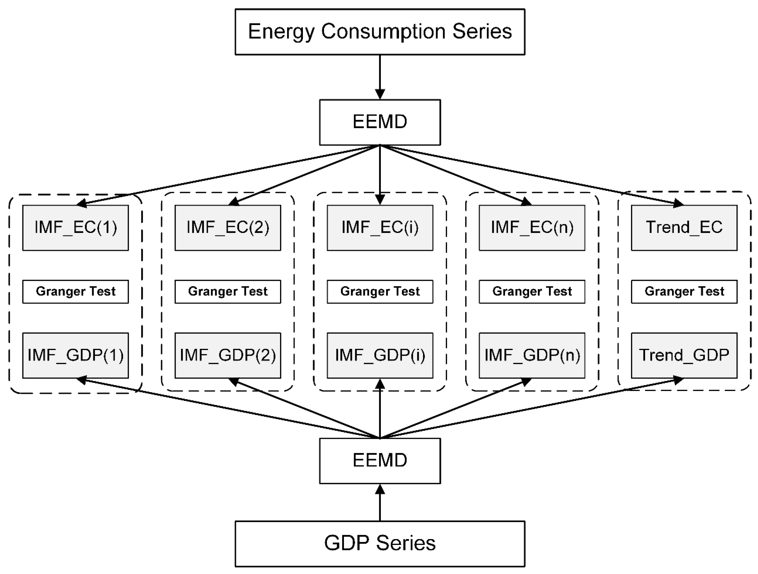
27] study, the VAR model and the error correction model were employed to test the short-run and long-run Granger causality relationships, respectively. Unlike their methods, in this research we attempt to decompose a time-series data into a trend component to denote the long-run trend of the time series. Subsequently, the decomposed trend component can be adopted to investigate the long-run causality relationship. To sum up, this study has two parts. One is to decompose the time series of growth rates of energy consumption and economic growth based on the EEMD method. The other is to estimate the short-run and long-run causality relationships between two decomposed time series obtained from the first stage by using the Granger causality test.
Furthermore, regarding the energy–GDP causality test, the literature has featured two different model specifications from the perspectives of the production function and the demand function. On the one hand, energy as an input factor like capital and labor can produce economic output, since neo-classical economic theory provides guidance on the causality relationship a priori. Hence, in the production framework, the more energy that is consumed, the greater the economic output and vice versa. Hence, a production function model, like the Cobb–Douglas production function, was constructed to test for the causality relationship [
32,
33]. On the other hand, economic development also causes consumption goods like energy consumption. Hence, a demand model including energy price was used to test for causality relationship since an energy price can signal the scarcity of an energy source [
34,
35]. Similarly, a bidirectional causality relationship would be expected since higher economic levels cause more energy consumed and vice versa. Many researchers are more interested in the demand causality model. However, the biggest challenge is a lack of energy price data. Alternatively, for Chinese studies, indices of raw materials, fuel and power are usually used to indicate the variable of energy prices. However, the data has been recorded only since the year 1990. In other words, the data is insufficient for this study. Most importantly, energy prices are tightly controlled in China so these cannot signal the scarcity of energy sources in China’s market economy. Hence, in this study we follow Liddle and Lung [
36] to employ a reduced form in order to examine the Granger causality relationship.
This study has three merits. The first is that we focus on the growth rate of energy consumption instead of the amount of energy consumption, since this conceals much useful information, for example, intrinsic fluctuations. The second is that we can obtain the long-run trend of the growth rate of both energy consumption and economic growth by means of the EEMD method. The last is that we provide a novel insight into the short-run and long-run Granger causality relationships between the two variables by performing the multi-timescale Granger causality tests, unlike the traditional VAR models and error correction models (ECM). To sum up, this study may help to better understand the causality relationship from a multi-timescale point of view.
The structure of this paper is arranged as follows.
Section 2 presents methods used in this research and data sources;
Section 3 exhibits empirical results and analyses; while
Section 4 draws conclusions and proposes a series of implications.
3. Empirical Results
3.1. EEMD Results
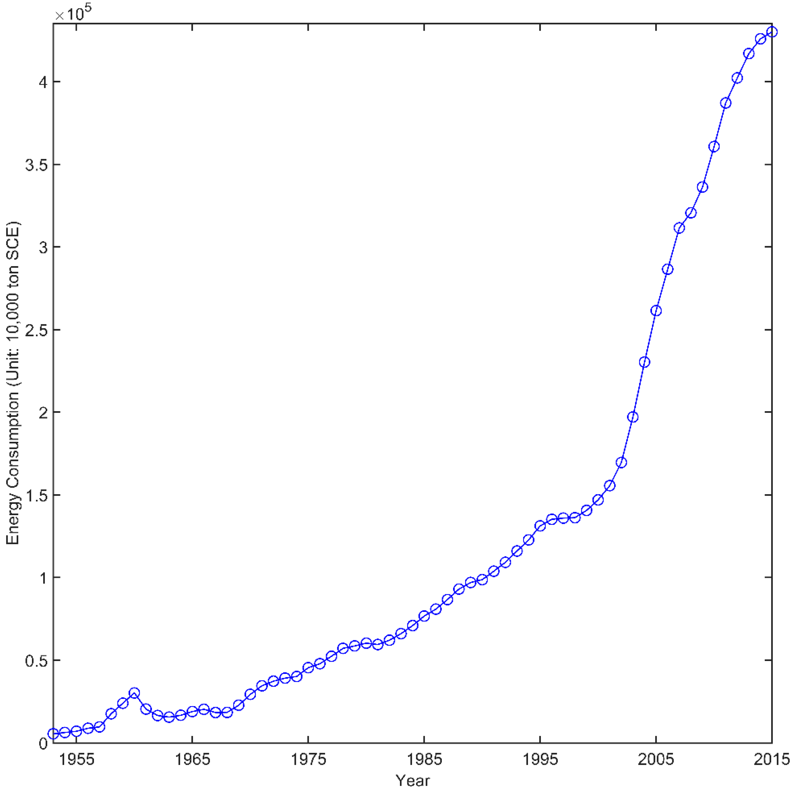
Figure 2 shows that the growth rate of energy consumption fluctuates over time. Hence, we will conduct the EEMD method to unravel the dynamic or periodic characteristics of the growth rate of energy consumption on multi-timescales. The EEMD method is suitable for decomposing the growth rate of energy consumption (
EC) in an effort to find out the intrinsic characteristics on multiple timescales.
We set the ensemble number as 100 as suggested by Bai et al. [
38] and Xu et al. [
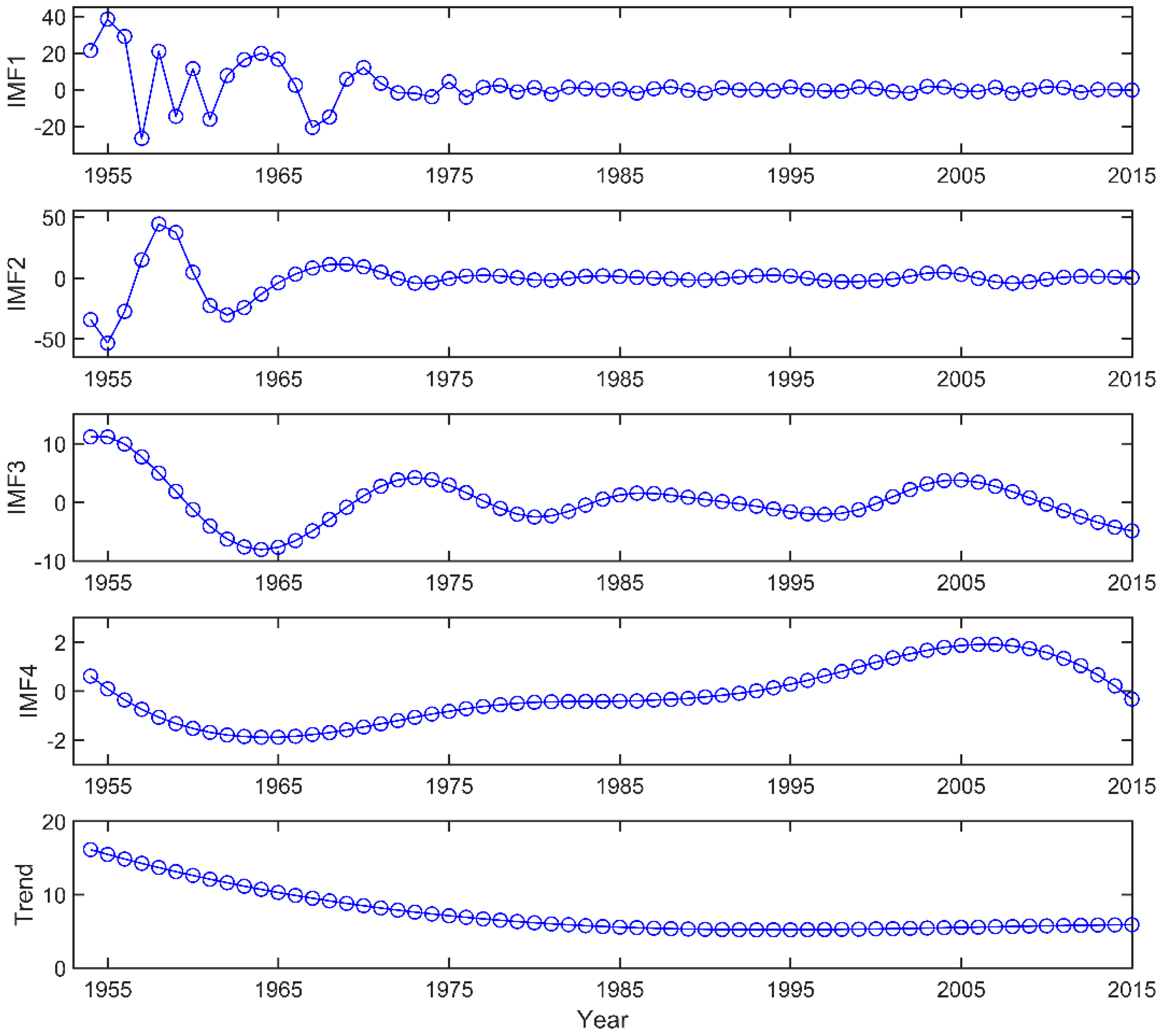
39]. The added white noise has an amplitude, specifically 0.2 times SD of the corresponding data. The decomposition of the
EC variable by using the EEMD method leads to four IMF components and a trend component. They are shown in
Figure 4.
Figure 4 shows each IMF component. Each of them has its own physical meaning. In other words, IMF1 to IMF4 components reflect the fluctuation characteristics in descending order, specifically from high to low frequency on different timescales. Specifically, IMF1 presents the highest-frequency oscillation and IMF4 the lowest-frequency oscillation. In addition, the residua series presents a U-shaped curve that indicates the overall trend of growth rates of energy consumption in China from 1954 to 2015. Specifically, it first decreases over time, reaches the nadir in 1993, and then increases over time. In other words, the year 1993 is the turning point. Additionally, the period and variance of each IMF component are summarized in
Table 1.
As shown in
Figure 4 and
Table 1, IMF1 and IMF2 are of high-frequency oscillation and have shorter periods (namely, IMF1 and IMF2 components with mean periods of about 3 years and 7.6 years, respectively) than low-frequency IMF3 and IMF4 (IMF3 and IMF4 components with mean periods of 12.2 and 53.7 years). Each IMF component clearly presents not only regular variation characteristics on different timescales under external forces but also the non-linear feedback of the energy–economy system.
Besides, these IMF components present not only periodic fluctuations, but also different variances. As shown in
Table 1, the variance of each IMF component for the growth rate of energy consumption is presented. It can be found that IMF1 and IMF2 components combined, accounting for 90%, have greater contributions than IMF3 and IMF4 components. In other words, there is little actual physical information embodied in IMF3 and IMF4 components. We place emphasis on IMF2 with about a 7.5-year period, since it accounts for about 60% of the growth rate variance. As shown in
Table 1, IMF2 has the highest Pearson correlation coefficient (0.530) with the original series data. Coincidentally, it corresponds to 1.5 times the length of the Five-Year Plan (five years) in China. In other words, the growth rate in a period of a Five-Year Plan may be not only be attributed to last year, but also will last until next year. To conclude, the Five-Year Plan policy may be the major influencing factor affecting China’s energy consumption.
Of greater interest is the overall trend. A turning point occurred in 1993. Coincidentally, in 1992 China’s energy consumption outpaced domestic energy production, with a deficiency of 19.14 million tons standard coal equivalent (SCE). As shown in
Figure 5, the energy deficit has been widening rapidly since 1993. Since then, China has been increasingly dependent on imports of energy, for example oil. In other words, using the EEMD method, we find that the growth rate of China’s energy consumption has been continuously increasing since 1993.
It is of great interest to us to examine if there exists Granger causality relationships between GDP and energy consumption. However, the relationship on multiple timescales has received little attention so far. Hence, in this study we attempt to fill this gap.
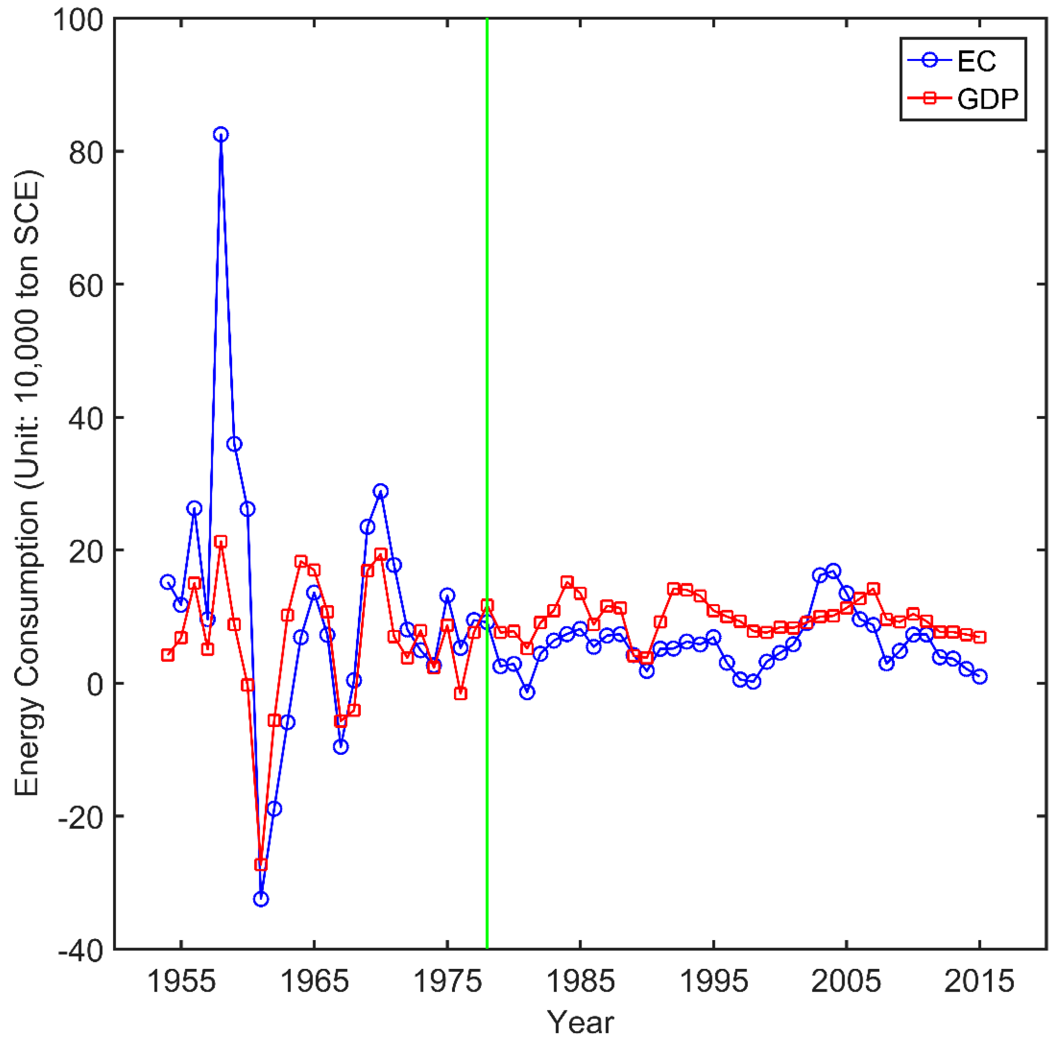
Before decomposing the growth rate of economic growth (GDP), we compare the growth rates of energy consumption and GDP. As shown in
Figure 6, before 1978 when China’s reform and opening-up policy was implemented, the growth rate of energy consumption outpaced the growth rate of GDP. After 1978, this development pattern reversed. From the above analysis, it follows that the policy contributed to China’s economic growth. The faster economic growth implies ever-decreasing energy intensity (energy intensity is defined as energy used to generate a unit of economic output) after 1978. However, it still lags behind that of advanced industrialized countries such as, Japan, Germany and the U.S.
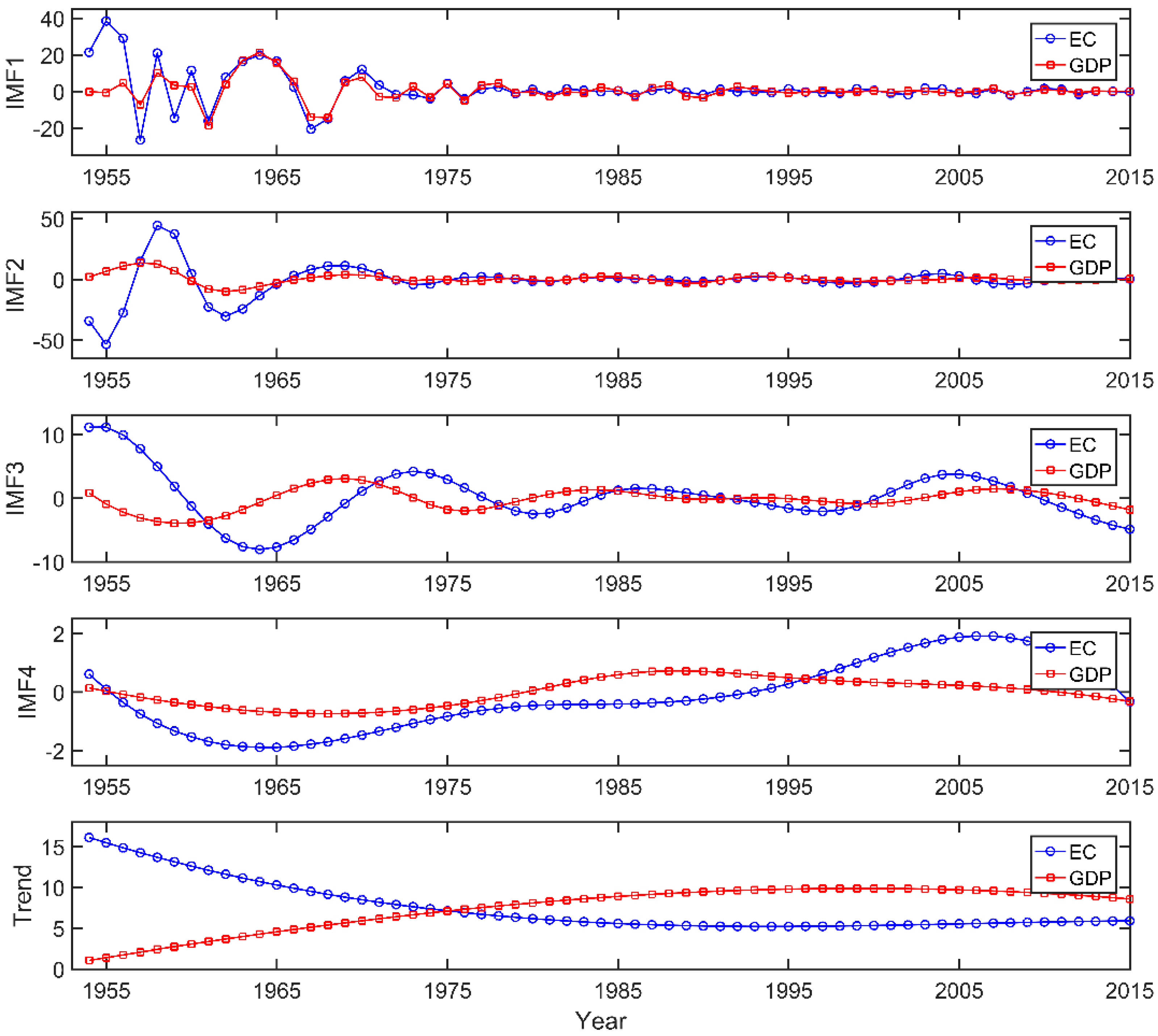
Next, we repeated the EEMD procedure for the growth rate of GDP. Consequently, four IMF components and a trend were also obtained. For simplicity, we define the five components as IMF1_GDP, IMF2_GDP, IMF3_GDP, IMF4_GDP and Trend_GDP. For the purpose of comparison, they are plotted in
Figure 7.
As shown in the first subfigure of
Figure 7, IMF1_GDP presents a similar pattern with IMF1_EC, particularly after 1957. Similarly, as shown in the second subfigure, IMF2_GDP has the similar fluctuation pattern. Regarding IMF3 and 4, they have different fluctuations. Finally, we pay considerable attention to the trend components. We find that Trend_GDP has a completely different development curve from Trend_EC. In other words, the growth rate of GDP first increases and then declines gradually. In particular, Trend_GDP outpaced Trend_EC in 1976, close to the year of 1978 when the reform was implemented. To sum up, we find that the four IMF GDP components have very similar oscillations and corresponding periods with IMF components for
EC.
3.2. Unit Root Test Results
Before moving to the Granger causality test, we performed the augmented Dickey Fuller unit root test (ADF test) for IMF1_GDP, IMF2_GDP, IMF3_GDP, IMF4_GDP, IMF1_EC, IMF2_EC, IMF3_EC and IMF4_EC time series, respectively, in order to verify if they were stationary.
Figure 7 shows that each IMF component seems to fluctuate up and down around zero during the sample period. Hence, no intercept and no trend are considered when testing for unit roots. The ADF test results are shown in
Table 2.
As shown in
Table 2,
t statistics for
θ are reported, followed by the critical values for the
t test at the 1%, 5% and 10% significance level. From the second to fifth row,
t statistics for all IMF components for energy consumption are less than the critical values at the 10% significance level, indicating that the null hypothesis is strongly rejected. In other words, IMF1 to 4 components for energy consumption are found to be stationary. Similarly, from thesixth to ninth row, all IMF components for GDP are stationary. To sum up, the ADF test results show that each IMF component time series has no unit root, or I(0).
3.3. Granger Causality Test Results
Finally, we conducted the Granger causality test for IMF1_EC and IMF1_GDP, IMF2_EC and IMF2_GDP, IMF3_EC and IMF3_GDP, IMF4_EC and IMF4_GDP, and Trend_EC and Trend_GDP in pairs, respectively. Since causality test results are very sensitive to the length of lags, the appropriate lags can be determined by using some criterion, for example, the Akaike information criterion (AIC), Schwartz criterion (SC), etc. Hence, in this study the AIC statistic is adopted to select the length of lags. More specifically, the smaller the AIC statistic is, the better it is fitted. These Granger causality test results are summarized in
Table 3.
In the context of IMF1, it can be found that there exists a bidirectional Granger causality relationship between GDP and EC. Similarly, in the context of IMF2, a bidirectional Granger causality relationship is also found. Although IMF3 and IMF3 made little contribution to explaining the time series, they reflect how these time-series change in the longer run. We still provide the Granger causality test results. In the context of IMF3 and IMF4, a unidirectional relationship running from GDP to EC indicating that in the longer run the growth rate of energy consumption is driven by the growth rate of economic growth. Last but not least, we repeat the ADF unit root test for Trend_EC and Trend_GDP time series to investigate if they are stationary. The results show that they have no unit roots. Subsequently, we performed the Granger causality test. As shown in
Table 3, there is a unidirectional causality relationship running from GDP to EC in the long run.
To sum up, there exists a short-run bidirectional Granger causality relationship between economic growth and energy consumption and a long-run unidirectional causality relationship running from economic growth to energy consumption. This reason may lie in two aspects. In the short run, China’s economy grows rapidly depending on the large scale of the development of industry, which leads to more energy being used. In the reverse direction, a great deal of energy consumption sustains the rapid development of industry, which in turn contributes to China’s rapid economic growth. Hence, industry plays a substantial and mediating role in the energy–economy system. In the long run, economic growth is the solo driving factor of energy consumption. On the one hand, China’s rapid and continuous economy growth stimulates energy production and energy consumption. In particular energy consumption signals if the economy increases and declines. If the growth rate of GDP declines, demand for energy also decreases, and energy production in turn shrinks. On the other hand, as the economy grows, income levels and living standards increase. A large number of energy-intensive products and services like cars, air-conditioners, and central heating systems etc. are consumed, which causes higher energy consumption. In other words, a large amount of energy cannot be consumed without continuous and rapid economic growth.
Moreover, there may be an extended explanation of the relationship between energy consumption and economic growth. This causality relationship discloses the nexus of energy matters and the economy. Sufficient energy supply is imperative for sustainable economic development since energy powers industrial systems. Moreover, various goods, for example, private cars, and services, for example, central heating systems, are also highly dependent on energy as income levels increase. To sum up, energy is of vital importance not only for production but also for consumption in the economy. On the other hand, a highly energy-dependent economy may cause environmental degradation that will affect sustainable development. Hence, for sustainable economic development an appropriate and harmonious relationship between energy consumption and economy is required.
4. Conclusions
In this paper, we revisited the Granger causality relationship between economic growth and energy consumption in China from a multi-timescale perspective. In the first stage we analyzed the characteristics of the annual growth rate of China’s energy consumption from 1954 to 2015 by means of the EEMD method. Four intrinsic mode function components with different periods on different timescales and an overall trend component were obtained from the decomposition method. An important finding from the overall trend component is that the year 1993 was the turning point for energy consumption growth, coinciding with the moment China’s energy consumption outpaced its energy production. Furthermore, China’s energy consumption gradually grew after 1993 and will keep increasing in the future. Then, we repeated the same procedures for the growth rate of China’s economic growth. Similarly, four IMF components and an overall trend were also obtained. In the second stage we performed the Granger causality test on different timescales. The results showed that there exists a short-run causality relationship running from GDP to energy consumption, and vice versa, and a long-run unidirectional causality relationship running from GDP to energy consumption.
These conclusions enable us to obtain a series of economic, social, and ecological implications. Firstly, energy must be the first priority in China’s economic growth since its economy heavily depends on energy sources. Since 1992, China’s energy consumption has outpaced its production, turning China into one the largest energy importers, especially of oil. Energy shortages seriously affect China’s sustainable development. To address the problem, China has expanded sources of energy imports. On the other hand, China’s central government has made great efforts to improve energy efficiency in a bid to balance the relationship between rapid economic growth and the potentially huge energy gap. Hence, a harmonious relationship between energy consumption and the economy is urgently required. Secondly, Chinese society is also heavily dependent on energy use. As income levels increase, a massive number of energy-intensive products and services, for example, private vehicles and central heating, are in demand in China leading to the consumption of a great deal of energy. To sustain better living standards, energy is one of the most indispensable prerequisites. Finally, since China has been experiencing rapid economic growth various pollutants caused by high energy consumption have led to serious environmental deterioration and even ecological disasters. For instance, a large scale of haze and fog events caused by coal combustion frequently occur in most areas of China. Moreover, China is also facing major challenges of water and soil pollution. Overdependence on energy consumption for the Chinese economy has posed a great threat to the country’s sustainable development and ecological environment. Hence, improvements in energy efficiency, the reduction of energy use and the pollutants this causes are urgently needed in order to develop an environmentally friendly society and sustainable development.


