An Integrated Carbon Policy-Based Interactive Strategy for Carbon Reduction and Economic Development in a Construction Material Supply Chain

Abstract

Carbon emissions from the construction material industry have become of increasing concern due to increasingly urbanization and extensive infrastructure. Faced with serious atmospheric deterioration, governments have been seeking to reduce carbon emissions, with carbon trading and carbon taxes being considered the most effective regulatory policies. Over time, there has been a global consensus that integrated carbon trading/carbon tax policies are more effective in reducing carbon emissions. However, in an integrated carbon reduction policy framework, balancing the relationship between emission reductions and low-carbon benefits has been found to be a critical issue for governments and enterprises in both theoretical research and carbon emission reduction practices. As few papers have sought to address these issues, this paper seeks to reach a trade-off between economic development and environmental protection involving various stakeholders: regional governments which aim to maximize social benefits, and producers who seek economic profit maximization. An iterative interactive algorithmic method with fuzzy random variables (FRVs) is proposed to determine the satisfactory equilibrium between these decision-makers. This methodology is then applied to a real-world case to demonstrate its practicality and efficiency.

1. Introduction

The “low carbon” concept was introduced at the World Climate Change Conference in Copenhagen, Denmark, 2009, after which low carbon economies became the major focus in many countries, leading to the development of the green supply chain (GSC) [1]. As one of the industries with the highest carbon emissions, the construction sector accounts for over one-third of global carbon dioxide emissions [2,3,4,5]. In addition to the carbon emissions from the daily operation of buildings, China has been undertaking many urban construction projects [6], which has led to a tremendous rise in construction carbon emissions [7]. In particular, as one of the six largest energy-consuming industries in China, the construction material industry represents 9% of the total energy consumption and 6% of total electricity consumption in China [8]. It is also a pillar industry in China since its added value makes up about 1% of the gross domestic product (GDP) each year [9]. The construction material industry has great potential with respect to energy conservation and carbon dioxide emission reduction, which could be of great significance to the achievement of total energy consumption control and transformation of low-carbon development. Enterprises, as the basic elements in the supply chain (SC), are required to take responsibility for the environmental performance of the supply chain participants [10]. As enterprises in supply chains are closely related, all are simultaneously affected by any carbon emission regulations. Therefore, SC enterprises must jointly adjust their operating and production plans to effectively achieve individual environmentally friendly performance [1]. Several advantages of the GSC have been identified, such as a positive corporate image, improved efficiency, and innovative leadership [1], all of which have encouraged more decision-makers to embrace GSC management (GSCM). When carbon emission regulations are imposed in a marketplace, scientifically designed environmental plans can enhance innovation, reduce total production costs, and highlight enterprise value [11]. Therefore, for each GSC member, low-carbon operations can represent a valuable, non-substitutable advantage [12]. Further, GSCM is a means for reducing potential losses from poor carbon emission performance that can intensify regulatory pressures [13], damage an enterprise’s image, attract government fines, and lead to customer boycotts or order cancellations [14,15].

At the same time, the focus on the protection of benefits in environmentally-related construction issues has grown, becoming a primary norm for the development of socioeconomic policies [16,17,18]. Therefore, further environmental policies and institutional acts on this topic are urgently required for greener approaches in the area of construction engineering [19]. Governments around the world have promulgated various policies to reduce carbon emissions, with carbon trading and carbon taxes considered the most effective policy schemes for reducing carbon emissions [20,21]. Carbon trading, which is a mainstay in emission trading programs, is specifically aimed at reducing carbon emissions [22]. In the carbon trading market, enterprises which want more than their allocated carbon emissions can purchase rights to emit more, and firms who do not require their allocated carbon emissions can sell their carbon emission rights to other enterprises [22]. There has been a sharp rise in the number of carbon emission trading schemes in recent decades. For example, in 2005, 374 million t of equivalent carbon dioxide were exchanged, but by 2011, the carbon trading volume had risen to 10.28 billion CO${}_2$ t, with the global carbon trading market valued at 176 billion US dollars [23]. Carbon taxes, which are a type of Pigovian tax [24], are a potentially cost-effective method for reducing greenhouse gas emissions [25]. Many European countries, such as the Netherlands, Sweden, Finland, and Norway, implemented carbon taxes many decades ago [26]. However, the Chinese government only introduced a carbon tax around 2013, which has severely affected the domestic market in China [27].

As stated above, most scholars have tended to study GSC from government or enterprise perspectives; however, while there have been many studies on carbon trading and carbon tax, many have only focused on the impact of a single policy on the macroeconomic development of carbon emission reductions, and the mutual relationships between supply chain enterprise operations and government policies have been ignored. In addition, there has been a lack of research on the performance of integrated carbon trading and carbon tax policies. To address this research gap, this paper explored the government and SC producer carbon reduction problems associated with integrated carbon trading and carbon tax policies. The government initially determines the annual free carbon emission allowances for the producer based on the average carbon emission level of the industry and its historical emission data. To control total carbon emissions and reduce the adverse impact of carbon emission reduction, the government, whose objective is to maximize social welfare, imposes a carbon tax on the producers. Under the dual constraints of emission allowance and carbon tax, the SC producers must be allocated sufficient carbon emissions to satisfy their daily operations. As the SC producers cannot exceed emission allowance limitations, they must either trade any remaining carbon emission allowances on the carbon trading market or directly purchase additional allowances to meet their emissions requirements. However, now carbon tax and the consumer’s low-carbon preference must be taken into serious consideration, while at the same time considering the carbon tax and consumer preference for low-carbon operations. Producers can achieve emission reductions by flexibly combining emission reduction investments and emission rights purchasing. Finally, to maximize their own profits, the SC producers must weigh up the emission costs and benefits under different strategy combinations to determine the final emission level and the associated product prices.

Because of the multiple decision-makers and the complex interactions, bi-level mathematical programming is proposed as it can accurately describe the interests of the decision-makers. Bi-level models have been widely applied in SC management [28,29,30,31,32]. For example, Ghosh and Shah [28] developed a bi-level supplier/manufacturer SC to examine SC coordination issues under a carbon emission policy. Song and Leng [29] included the carbon emission factors into a single-cycle newsboy model to examine the influences of different carbon emission policies on producers’ orders. Choi [30] examined the impact of a carbon footprint tax on bi-level fashion SC systems, and the importance of the carbon footprint tax on SC fashion management. Du et al. [31] considered an emission-dependent SC to examine an emission-dependent manufacturer and an emission permit supplier under a cap-and-trade system. Jaber et al. [32] researched bi-level manufacturer/retailer SC game processes and coordination mechanisms under carbon cap-and-trade conditions.

These studies have inspired researchers with novel management insights into government carbon emission regulations and GSC operations; however, the carbon emission regulation parameters have been generally regarded as exogenous variables, with the governments not being involved in the decision-making processes. Therefore, the main contributions of this paper are as follows. First, the integration of carbon reduction policies and their relationships within GSCs are explored. Second, optimal decision results are theoretically derived through the development of a bi-level optimization model, in which the leader, which has a social welfare maximization objective, determines the carbon tax and emission allowance allocations, and the following producers, which have a profit maximization objective, determine their production output and sales quantities. Third, it is shown that the sustainable GSC development and a trade-off between environmental protection and economic development can be achieved by employing the proposed methodology.

The remainder of this paper is organized as follows. Section 2 gives the research and problem statement, including the research background and the decision-making relationship analysis. In Section 3, a methodology, including a bi-level mathematical model and an interactive algorithm, is established as an abstraction of the real problem. To confirm the generality of the methodology, a general case, results, and some further discussions are given in Section 4. Finally, Section 5 gives the conclusions and suggestions for future studies.

2. Research and Problem Statement

In an integrated carbon policy-based carbon emission reduction problem, there are various decision-makers: the government as the leading decision-maker and the GSC producers as the following decision-makers who act based on the government’s decisions. Both parties have individual contradictory carbon reduction targets. The government seeks to effectively reduce overall carbon emissions, while safeguarding the economic interests of the producers, with the aim of stimulating participation and enthusiasm for emission reduction, and maximizing total social welfare, while the producers seek to obtain as high a carbon emission allowance as possible to reduce their emission costs and maximize profits. Both of parties have individual but interacting decision-making variables; the government’s decision-making variables are the free carbon emission allowances and the carbon tax; while the producer’s variables are production and sales quantities. It is assumed that the GSC producers have an equal market position and each independently trades their carbon emission allowances on the open market. As the producers’ profits are considered when the government sets the carbon emission reductions targets, the decisions made by the producers not only determine their own objectives but also influence the government’s goals. Therefore, the government’s decisions also need to consider the influence of the producers’ responses to its own goals. Therefore, the carbon emission reduction problem in this paper is a dynamic optimization decision-making process, within which the government needs to monitor the carbon trading market, assess the effectiveness of the carbon tax level, and improve their emission reduction strategies based on the responses from the market and the producers.

The above analysis has shown that the carbon emission reduction decision-making process is an interactive decision-making mechanism comprised of the government as the leading decision-maker responsible for the overall carbon reduction plan and control, and the producers as the following decision-makers who have independent decision-making rights in terms of their own carbon reduction goals. As the government is in the lead decision-making position, it has the advantage of moving first. From this description, this integrated emission reduction decision-making policy problem has the same characteristics and mechanisms as a general bi-level decision-making problem, which is similar to the hierarchical decision leader–followers Stackelberg game, in which the leader is more powerful and the follower reacts rationally to the leader’s decisions [33,34]. Therefore, the bi-level Stackelberg game can be used to examine this level of this government/producers carbon emission reduction decision-making relationship.

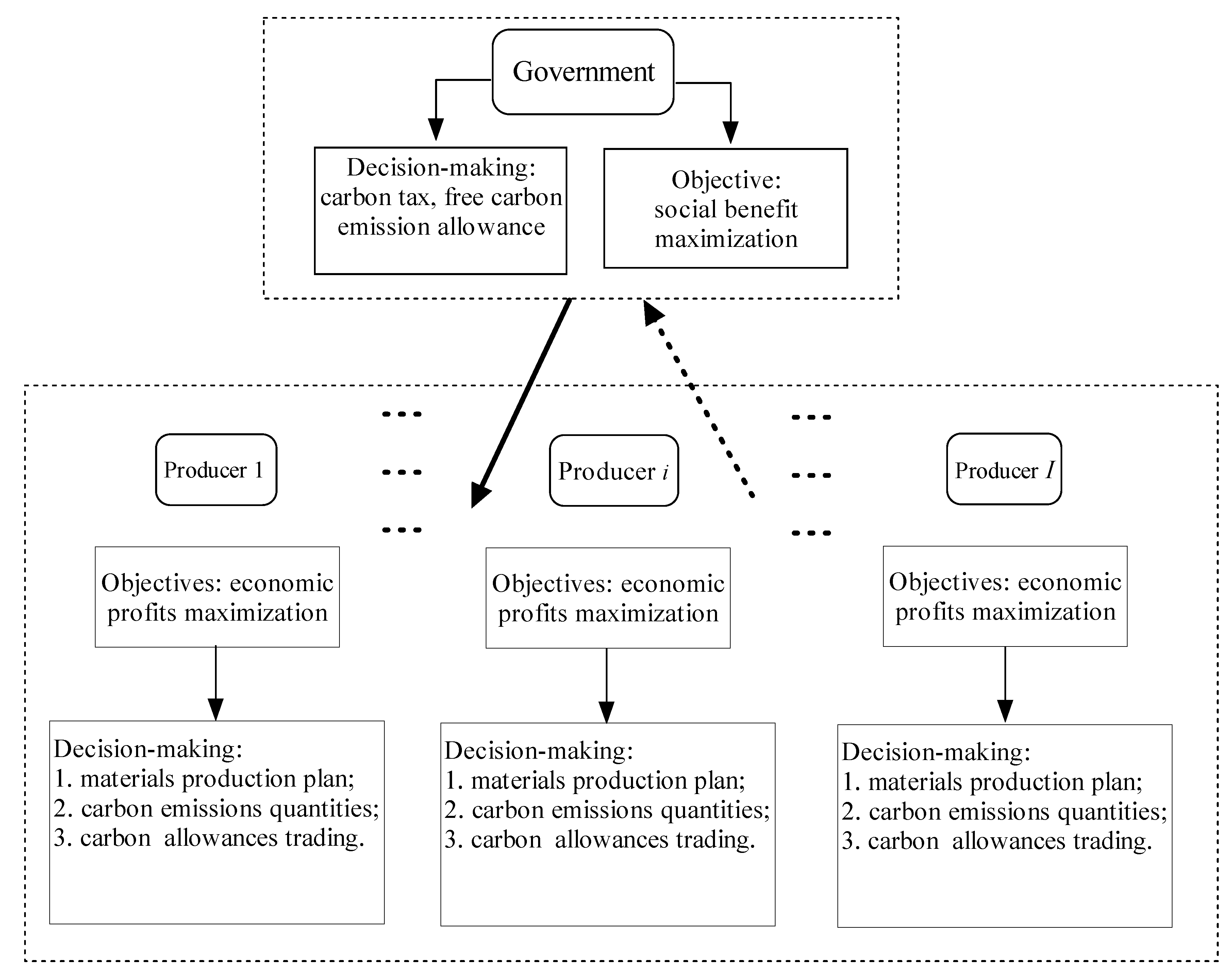
This problem can be abstracted as a bi-level mathematical model for calculation, which, along with the hierarchical structure makes it a complex problem, as shown in the concept model in Figure 1.

3. Methodology

A bi-level mathematical model and a corresponding solution approach are proposed in this section.

3.1. Bi-Level Programming

Assumptions, notations, objective functions and constraints of an integrated emission reduction decision-making policy problem are introduced in this section.

3.1.1. Assumptions

Before formulating the model, the following assumptions are given:

A${}_1$

This integrated carbon emission policy problem is a single-period decision-making problem; therefore, a static optimization problem is assumed.

A${}_2$

The government is responsible for the initial free carbon emission allowance allocation and the producers freely transact with other producers in the CET market.

A${}_3$

None of the producers can individually meet all the projects’ requirements [35].

A${}_4$

Each decision-maker fully understands the objective functions and inherent constraints, and behaves rationally [36].

3.1.2. Notations

Sets:

$\mathbb{I}$ :	Set of producers, $\mathbb{I}=\{1,2,\cdots ,I\}$.
$\mathbb{J}$ :	Set of projects, $\mathbb{J}=\{1,2,\cdots ,J\}$.

Indices:

i :	Index for the construction material producers, $i\in \mathbb{I}$.
j :	Index for the projects, $j\in \mathbb{J}$.

Decision variables:

${\alpha }_i$ :	Free carbon emission allowance for construction material producer i.
$\gamma$ :	Carbon tax rate for construction material production.
$q_i$ :	Total construction materials produced by producer i.
$q_{ij}$ :	Total construction materials purchased from producer i for project j.

Certain parameters:

$Cap$ :	Actual free carbon allowance allocation for the construction material industry in the last production period.
${\gamma }^l$ :	Lower bounds for the unit carbon tax.
${\gamma }^u$ :	Upper bounds for the unit carbon tax.
$C{E}_i^u$ :	Carbon emissions produced by producer i with no emission reduction measure.
$C{E}_i^l$ :	Carbon emissions produced by producer i after the carbon reduction efforts.
$P{C}_i$ :	Unit production cost for construction material producer i.
$I{C}_i$ :	Unit inventory cost for construction material producer i.
$P_{ij}$ :	Price of a unit of construction material k from producer i for project j.
$G{P}_i$ :	Production carbon emission coefficient for producer i.
$P{M}_i^l$ :	Lower bounds for the production capacity for producer i.
$P{M}_i^u$ :	Upper bounds for the production capacity for producer i.
$S{C}_i^{max}$ :	Maximum storage capacity of producer i.
$\beta$ :	Market price of carbon emission trading.
$\lambda$ :	Sale taxes an enterprise pays for a unit of construction material.

Uncertain parameters:

$\widetilde{\overline{D_j}}$ :

Total demand of project j for construction materials.

3.1.3. Model Formulation

This section gives a detailed description of the global model including the model of the government and the model of the producers.

Objective 1: The government’s social benefit objective. To balance the environmental protection and economic development of the construction material industry, the government must control carbon emissions while also considering the social benefits. However, the social benefits are the primary objective, which are made up of three parts; sales taxes on materials, revenue from carbon emission trading, and the carbon tax revenue. Let $\lambda$ be the unit sales tax for the construction material. The total sales taxes for the materials are therefore $\lambda {\sum }_{i=1}^I{\sum }_{j=1}^J{q}_{ij}$. It is assumed that $\beta$ is the carbon emission trading price. Therefore, the total carbon emission trading revenue is $\beta {\sum }_{i=1}^I\left(G{P}_i{q}_i-{\alpha }_i\right)$. Under the carbon tax policy, construction material producers have paid taxes for their carbon emissions. Let $\gamma$ be the unit carbon tax for producing the construction materials. The total carbon tax revenue is therefore $\gamma {\sum }_{i=1}^{I}G{P}_i{q}_i$, and the overall social benefit for the government is:

$$maxW=\lambda \sum _{i=1}^I\sum _{j=1}^J{q}_{ij}+\beta \sum _{i=1}^I\left(G{P}_i{q}_i-{\alpha }_i\right)+\gamma \sum _{i=1}^{I}G{P}_i{q}_i.$$

(1)

Constraint 1: Free carbon emission allocation constraint. To limit the carbon emissions, the government initially allocates free allowances to the producers. To protect the construction material industry, the government cannot allocate a carbon emission allowance beyond a producer’s capacity. Therefore, there exists an upper bound, $\le C{E}_i^m$, for producer i, which represents the maximum carbon emissions emitted when producer i is under full-load production; this constraint is denoted as ${\alpha }_i\le C{E}_i^m$. However, to guarantee each producer’s basic rights, the government must allocate a carbon emission allowance that ensures that the producer can produce at capacity. Therefore, there exists a lower bound, $C{E}_i^l$, for producer i, which is the minimum carbon emission allowance allocation needed to maintain basic operations. This constraint is denoted as $C{E}_i^l\le {\alpha }_i$. To ensure both sides are fully considered, the producers’ restrictions when the government makes decisions are:

$$C{E}_i^l\le {\alpha }_i\le C{E}_i^m.$$

(2)

Constraint 2: Industry free carbon emission allowance allocation constraint. As the government must guarantee the atmospheric environment, they may alter their intentions to control the carbon emissions of the whole industry within an acceptable range, which cannot surpass the actual free carbon allowance allocation given to the construction material industry in the last production period,

$$\sum _{i=1}^I{\alpha }_i\le Cap.$$

(3)

Constraint 3: Carbon tax constraint. The formulated unit carbon taxes must be within the minimum and maximum carbon tax limitation bounds, which can be expressed as:

$${\gamma }^l\le \gamma \le {\gamma }^u.$$

(4)

Constraint 4: Demand constraint. As construction materials are required to ensure the project meets its construction deadlines, the producers must satisfy the demand for each type of project material. However, because of the inherent complexity and uncertainty in construction technology as well as the fluctuating demand, accurate data for the material supply level is difficult to obtain. Therefore, this demand is dealt with using an expected value operator. The material quantities provided to each project, therefore, must satisfy the respective demands, namely,

$$\sum _{i=1}^I{q}_{ij}\ge E\left[\widetilde{\overline{D_j}}\right].$$

(5)

Objective 2: Producer’s profit objective. With the integrated carbon policies, each producer, as an independent decision-maker, seeks to maximize his individual profit, which is the difference between total revenue and total cost. Total revenue comes from construction material sales ${\sum }_{j=1}^J{P}_{ij}{q}_{ij}$, while total costs are made up of material production costs $P{C}_i{q}_i$, inventory costs $I{C}_i\left(q_i-{\sum }_{j=1}^J{q}_{ij}\right)$, sales taxes $\lambda {\sum }_{j=1}^J{q}_{ij}$, CET costs $\beta \left(G{P}_i{q}_i-{\alpha }_i\right)$, and carbon taxes $\gamma G{P}_i{q}_i$. Therefore, the profit function is:

$$max{P}_i=\sum _{j=1}^J{P}_{ij}{q}_{ij}-P{C}_i{q}_i-I{C}_i\left(q_i-\sum _{j=1}^J{q}_{ij}\right)-\lambda \sum _{j=1}^J{q}_{ij}-\beta \left(G{P}_i{q}_i-{\alpha }_i\right)-\gamma G{P}_i{q}_i.$$

(6)

Constraint 5: Producers’ carbon emissions constraint. The amount of carbon emissions for each producer cannot exceed the emissions without a reduction measure but must not be lower than the amount of emissions with the greatest carbon reduction efforts, that is,

$$C{E}_i^l\le G{P}_i{q}_i\le C{E}_i^m.$$

(7)

Constraint 6: Production capacity constraint. When providing construction materials for multiple projects, the material production $q_i$ of producer i must be within a specified range between the maximum and minimum production capacity. Therefore, the production capacity constraint is:

$$P{M}_i^l\le q_i\le P{M}_i^u.$$

(8)

Constraint 7: Inventory constraint. Each producer owns a warehouse for temporarily storing construction materials that are not yet sold. The construction material inventory level of producer i cannot exceed the storage capacity, namely

$$0\le q_i-\sum _{j=1}^J{q}_{ij}\le S{C}_i^{max}.$$

(9)

3.1.4. Global Model

To sum up, the global model is built as in Equation (10). The decision-makers impact on each other as the government’s decisions $\left({\alpha }_i,\gamma \right)$ affect the construction material producers’ decisions $\left(q_i,q_{ij}\right)$. The government attempts to expand the social benefit by reducing total carbon emissions, however, each construction material producer seeks profit maximization. At the same time, the producers’ actions $\left(q_i,q_{ij}\right)$ affect the government’s subsequent actions $\left({\alpha }_i,\gamma \right)$. Consequently, all decision-makers seek satisfactory solutions based on their respective optimization targets. At the beginning, based on previous information and its own objectives, the government determines the initial carbon emission allowance allocations, the decisions for which are then is delivered to the construction material producers. Each producer, as a follower, sets its own plan in view of the government’s decisions, the market demands, and their own technological conditions. The producers’ plans are then submitted to the government, after which the government adjusts its initial decisions in consideration of each producer’s emission performance, and an improved plan is then sent to the producers. Therefore, the government influences the behavior of the construction material producers without completely controlling their actions, and the construction material producers’ behavior affects the government’s decisions. Relationships between each construction material producer are also assumed to be non-cooperative, as each producer makes decisions independently and without collaboration [37]. Each producer, therefore, has an optimization problem, in which the other producers’ decisions are regarded as the certain parameters. Therefore, the problem can be expressed mathematically in a bi-level programming model. In summary, the global model is:

$$\begin{array}{c}maxW=\lambda \sum _{i=1}^I\sum _{j=1}^J{q}_{ij}+\beta \sum _{i=1}^I\left(G{P}_i{q}_i-{\alpha }_i\right)+\gamma \sum _{i=1}^{I}G{P}_i{q}_i\hfill \\ \mathrm{s}.\mathrm{t}.\left\{\begin{array}{c}C{E}_i^l\le {\alpha }_i\le C{E}_i^m\hfill \\ \sum _{i=1}^I{\alpha }_i\le Cap\hfill \\ {\gamma }^l\le \gamma \le {\gamma }^u\hfill \\ \sum _{i=1}^I{q}_{ij}\ge E\left[\widetilde{\overline{D_j}}\right]\hfill \\ max{P}_i=\sum _{j=1}^J{P}_{ij}{q}_{ij}-P{C}_i{q}_i-I{C}_i\left(q_i-\sum _{j=1}^J{q}_{ij}\right)-\hfill \\ \lambda \sum _{j=1}^J{q}_{ij}-\beta \left(G{P}_i{q}_i-{\alpha }_i\right)-\gamma G{P}_i{q}_i\hfill \\ \mathrm{s}.\mathrm{t}.\left\{\begin{array}{c}C{E}_i^l\le G{P}_i{q}_i\le C{E}_i^m\hfill \\ P{M}_i^l\le q_i\le P{M}_i^u\hfill \\ 0\le q_i-\sum _{j=1}^J{q}_{ij}\le S{C}_i^{max}\hfill \end{array}\right.\hfill \\ {\alpha }_i,\gamma ,q_i,q_{ij}\ge 0\hfill \\ i\in \mathbb{I},j\in \mathbb{J}\hfill \end{array}\right.\hfill \end{array}$$

(10)

3.2. Iterative Interactive Algorithm

As is well known, bi-level programming optimization is a non-deterministic polynomial (NP) hard problem even in its most common formulation [38,39,40]. The decision variables of the government’s upper-level mathematical model and the producers’ lower-level mathematical models are therefore nested in each decision-maker’s objective function and constraints of the model (10), for which an iterative interactive algorithm based on evolutionary game theory between the two decision-makers is established to deal with the complex model (10) interaction. The iterative interactive algorithm solves both the upper and lower optimization problems in the bi-level programming mathematical model. At first, all constraints in the government’s upper-level optimization model are set using Matlab R2013a (MathWorks, Natick, MA, USA) and a feasible zone of the upper-level optimization model is built. Then a vector $\left({\alpha }_i,\gamma \right)$ is generated, which is the initial solution to the upper-level optimization model, after which vector $\left({\alpha }_i,\gamma \right)$ is put into the lower-level optimization model as the constant, and the model is transformed into a single-level programming model for $\left(q_i,q_{ij}\right)$. By employing the mathematical toolbox in Matlab R2013a, an initial solution to the producers’ optimization model, $\left(q_i,q_{ij}\right)$, is obtained, which is fed back to the upper-level optimization model, and the model is also transformed into a single-level programming model for $\left({\alpha }_i,\gamma \right)$ for the government. The mathematical toolbox in Matlab R2013a is employed again to obtain an improved solution, $\left({\alpha }_i,\gamma \right)$. If the government is satisfied with the improved solution, the computation is terminated. If not, the new solution $\left({\alpha }_i,\gamma \right)$ is again imported into the lower-level optimization model and the solution to the model calculated, thus generating a new vector for $\left(q_i,q_{ij}\right)$, which is then conveyed to the upper-level model again. As an interactive mechanism in this bi-level decision-making structure, this process is repeated several times until an overall satisfactory solution to both the upper and lower level optimization models is obtained, which is the final solution to the proposed bi-level optimization model. The procedures for this solution approach are shown in Figure 2.

4. Case Study

In this section, the construction material industry in City X is employed as a practical case to probe into the integrated carbon emission reduction policy and to demonstrate the practicality of the proposed optimization methodology.

4.1. Case Description

Industry is the dominant consumer of energy and producer of ${\mathrm{CO}}_2$ emissions in China. China’s urbanization process has undoubtedly promoted infrastructure construction, which has stimulated demand for cement, ceramics, glass, and other construction materials [41]. The emission reduction potential is of great significance to the achievement of the total carbon reduction control. City X, the main region for cement production in Shanxi province, supplies the Shanxi province with 20% of its cement demands. The cement industry plays a key role in the economic development of City X, however, emissions from material production are the primary source of carbon emissions, and represent a serious menace to local air quality. In terms of air quality, City X has been judged as one of the worst cities in the Shanxi province. Thus, reducing carbon emissions in construction material industry is regarded as the primary goal for the local government in the next production period.

4.2. Data Presentation

In City X, three main cement producers, referred to as A, B, and C, are engaged in the production and supply of cement for three key projects, referred to as I, II, and III. The carbon trading price was set at 60 $\mathrm{CNY}/\mathrm{t}$ based on the average carbon allowance trading price at City X’s Emissions Trading Institution. The lower and upper bounds for the carbon tax rate were 10 $\mathrm{CNY}/\mathrm{t}$ and 30 $\mathrm{CNY}/\mathrm{t}$, respectively, based on the recommendations from National Development and Reform Commission experts. The unit sales tax for cement was 50 $\mathrm{CNY}/\mathrm{t}$, and the total carbon emissions in the last planning period $Cap$ were about $3.2\times {10}^6\mathrm{t}{\mathrm{CO}}_2$. Information for producers, such as the emission allowances, production capacity bounds, the carbon emission coefficient, production and inventory unit cost, maximum storage capacity, and unit prices, are listed in

Table 1. Basic information for the cement producers.

Parameters	Producer A	Producer B	Producer C
Lower bounds for carbon emissions (${10}^5$ t)	6.3	5.4	6.2
Upper bounds for carbon emissions (${10}^5$ t)	14.7	13.3	14.3
Lower bounds for production capacity (${10}^4$ t)	140	138	135
Upper bounds for production capacity (${10}^4$ t)	180	175	180
Carbon emission coefficient (kg CO${}_2$/t)	630	608	622
Unit production costs (CNY/t)	52	46	54
Unit inventory costs (CNY/t)	24	27	26
Maximum storage capacity (${10}^4$ t)	54	52	55
Unit price of cement for Project I (CNY/t)	290	305	296
Unit price of cement for Project II (CNY/t)	292	310	305
Unit price of cement for Project III (CNY/t)	280	300	286

. From Table 1, it is clear that the production costs were slightly higher for Producer B, but fewer emissions were generated due to the advanced, more efficient machinery and manufacturing technology. The cement demands for the three key projects are listed in

Table 2. Project demands for cement.

	Project I	Project II	Project III
Cement (${10}^4$ t)	$(135,\mathcal{N}(160,25),197)$	$(146,\mathcal{N}(172,18),196)$	$(126,\mathcal{N}(155,20),173)$

.

4.3. Results Analysis

By importing the collected data into the proposed optimization model (10) and running the iterative interactive algorithm on Matlab R2013a, the results for the proposed model were determined, as shown in

Table 3. Satisfactory solution.

Decision-Makers	$\mathit{\gamma }$	${\mathit{\alpha }}_{\mathit{i}}$	${\mathit{q}}_{\mathit{i}}$	${\mathit{q}}_{\mathit{ij}}$ $\left({\mathbf{10}}^{\mathbf{4}}\mathbf{t}\right)$			Social Benefits (Profits)
	($\mathbf{CNY}/\mathbf{t}$)	$\left({\mathbf{10}}^{\mathbf{5}}\mathbf{t}{\mathbf{CO}}_{\mathbf{2}}\right)$	$\left({\mathbf{10}}^{\mathbf{4}}\mathbf{t}\right)$	I	II	III	$\left({\mathbf{10}}^{\mathbf{8}}\mathbf{CNY}\right)$
Government	20	-	-	-	-	-	3.08
Producer A	-	9	147	55	50	42	2.56
Producer B	-	9.5	160	55	55	50	3.17
Producer C	-	11	180	50	67	63	3.24

. Satisfactory solutions were obtained for both the government and the producers, in which the social benefits for the government were estimated at $W=3.08\times {10}^8\mathrm{CNY}$, and the profits for Producers A, B, and C were respectively $P_A=2.56\times {10}^8\mathrm{CNY}$, $P_B=3.17\times {10}^8\mathrm{CNY}$, and $P_C=3.24\times {10}^8\mathrm{CNY}$. The total carbon emission allowance for the construction material industry for the government was $29.5\times {10}^5\mathrm{t}{\mathrm{CO}}_2$, of which $9\times {10}^5\mathrm{t}{\mathrm{CO}}_2$, $9.5\times {10}^5\mathrm{t}{\mathrm{CO}}_2$, and $11\times {10}^5\mathrm{t}{\mathrm{CO}}_2$ were allocated to Producers A, B, and C, respectively. The optimal carbon emissions for Producers A, B, and C were $9.26\times {10}^5\mathrm{t}{\mathrm{CO}}_2$, $9.72\times {10}^5\mathrm{t}{\mathrm{CO}}_2$, and $11.20\times {10}^5\mathrm{t}{\mathrm{CO}}_2$, respectively, and extra carbon emission allowances were purchased from the government.

4.4. Carbon Tax Analysis

In this section, different values for the carbon tax were set to verify its influence on the overall and individual emissions and economic performances, in which the $\gamma$ ranged from 10 to 30 $\mathrm{CNY}/\mathrm{t}$ in intervals of 5 $\mathrm{CNY}/\mathrm{t}$. Figure 3 and Figure 4 show the influence of the different values for the carbon tax on industry carbon emissions, social benefits, and profits for the government and Producers A, B and C.

In Figure 3, as the carbon tax increased, the total carbon emissions in the construction industry continued to decrease, and when $\gamma \ge 20\mathrm{CNY}/\mathrm{t}$, the total emissions were less than the government’s annual emission objectives (i.e., $29.5\times {10}^5\mathrm{t}{\mathrm{CO}}_2$). This indicated that the a carbon tax policy could be a good carbon emission reduction method. From the producers’ perspective, with an increase in the carbon tax, the carbon emissions of Producers A and C decreased; however, the carbon emissions of Producer B increased, indicating that Producer B was a lower carbon emission enterprise than the other two producers. When the government imposed stricter carbon tax regulation, consumers tended to purchase materials from Producer B to avoid the carbon tax being passed on. Therefore, Producer B was able to produce a greater number of materials than previously, thereby generating greater carbon emissions.

In Figure 4, as the carbon tax grew, the government’s social benefits and Producer B’s profits increased, and the growth rates of both when $\gamma \in [20,30]$ were obviously larger than when $\gamma \in [10,20]$. Because the increased carbon tax revenue raised social benefits, the promoted projects purchased more materials from Producer B. However, under the pressure of a higher carbon tax, Producers A and C had to reduce their production output, leading to a decrease in profits. From the producers’ perspective, when faced with different carbon tax changes, enterprises with lower carbon emissions would be more favored by the government and the market, and enterprises with higher carbon emissions would need to improve machinery and invest in cleaner manufacturing technology. From the industry perspective, total profits were relatively unchanged, which indicated that the carbon tax policy had little negative impact on the economic development of the construction material industry.

4.5. Comparative Analysis in Different Decision-Making Environments

The computational results were acquired by employing some fuzzy random variables (FRVs) under a fuzzy random environment; however, the results may alter in different decision-making environments. To measure the robustness of the methodology when some parameters from model (10) had some perturbations, a sensitivity analysis was conducted to demonstrate the effect on the solutions under different decision-making environments. First, model (10) under a fuzzy random environment was compared to a model under a certain environment, in which the mean values for the FRVs were kept to eliminate uncertainty in the determined environment. For example, for the demands for Project I (i.e., $\widetilde{\overline{D_I}}=(135,\mathcal{N}(160,25),197)$), the adopted value was 166, which was the mean value from 135 and 197. The computational results are shown in

Table 4. Results comparison for the government in model (10) under different environments.

Objective	Unit:	Fuzzy Random	Certain	Fuzzy
	${\mathbf{10}}^{\mathbf{8}}$ CNY	Environment	Environment	Environment
	Best	3.34	3.38	3.32
W	Average	2.95	2.86	2.94
	Worst	2.65	2.45	2.52

. Second, model (10) under a fuzzy random environment was also compared to a model in a fuzzy environment, in which in the fuzzy environment the fuzziness in the FRVs was retained, but the stochastic nature was neglected. To obtain useful data, Gaussian distributions were removed and the expectations were reserved. For instance, the demands of Project I in the fuzzy environment were denoted as $(135,160,197)$. The expected method was also used to convert the objective functions into equivalent crisp functions. The comparative results are also shown in Table 4.

The results in Table 4 indicated that the solutions in the determined environment had greater deviations than those in the fuzzy random environment, indicating that model (10) under a fuzzy random environment was able to provide more reliable references for the decision-makers. It was also found that the results under the fuzzy random environment were also better than in a fuzzy environment. Therefore, the proposed methodology was found to be robust in solving a carbon emission reduction problem for the construction material industry for the government, and the use of the fuzzy random environment was better able to match actual circumstances based on the post hoc analysis.

5. Conclusions

Carbon emission reduction is important to the sustainable development of the construction material industry. Most construction material activities, such as material producer selection, material production plans, dynamic inventories, and assignment problems, are interrelated, which means that contradictions between the government and construction material enterprises are unavoidable. Previous research has demonstrated that to achieve sustainable development in the construction material industry, these contradictions need to be reduced or fully resolved [2,4,36,42].

However, research on carbon emission reduction problems in the construction material supply chain has been restricted to a simple overall GSC system, or only a single carbon emission policy was assumed. Therefore, there were several difficulties that remained unresolved. Firstly, the hierarchical decision-making relationships between the government and the producers were not considered; however, as there are multiple stakeholders within this structure, contradictions must be considered. Secondly, linearization assumptions and simplifications were often employed to ensure model tractability, which led to loss of generality in the mathematical models. Thirdly, uncertainty and complications in the decision-making environment were not considered when dealing with the collected data.

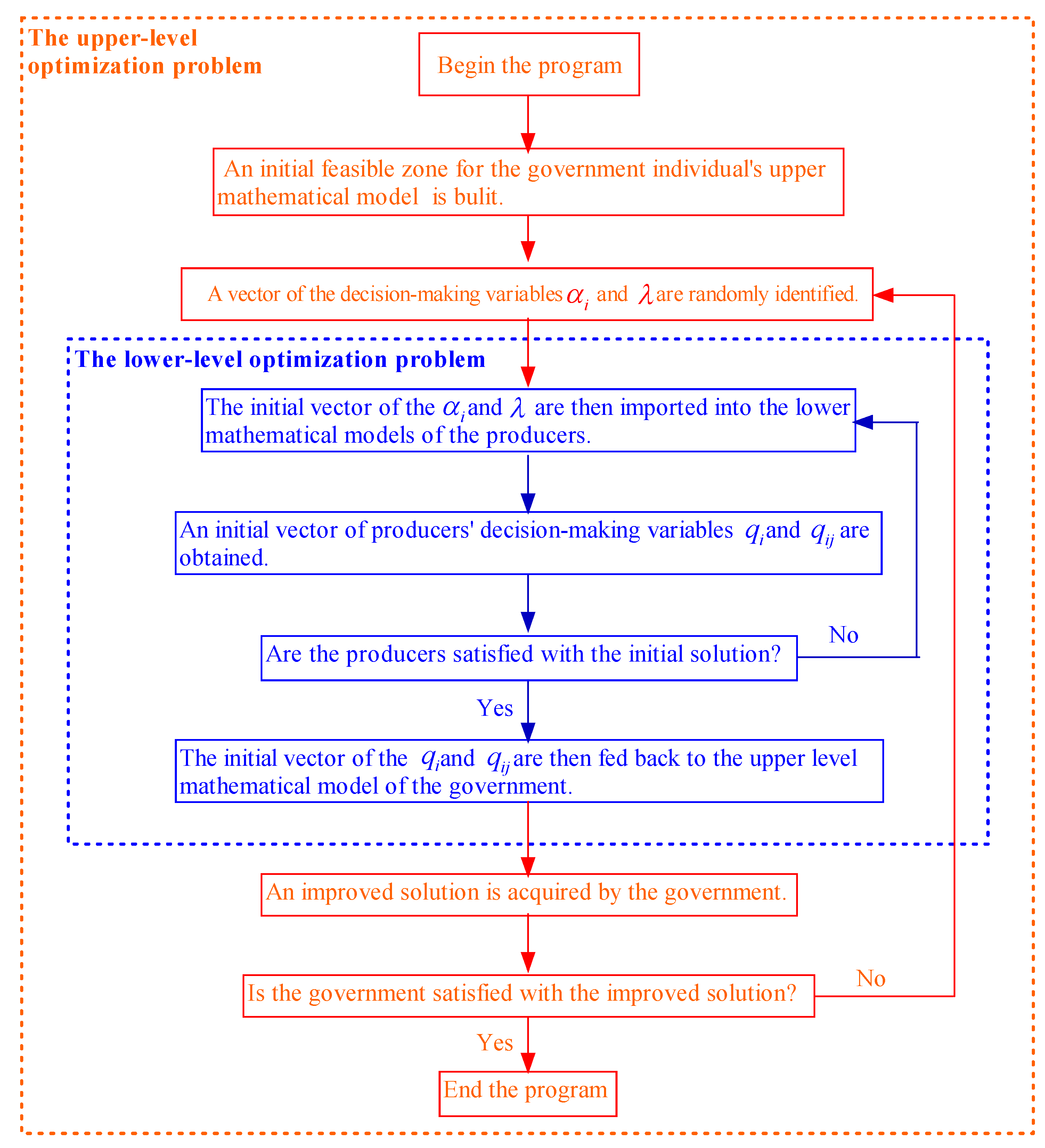
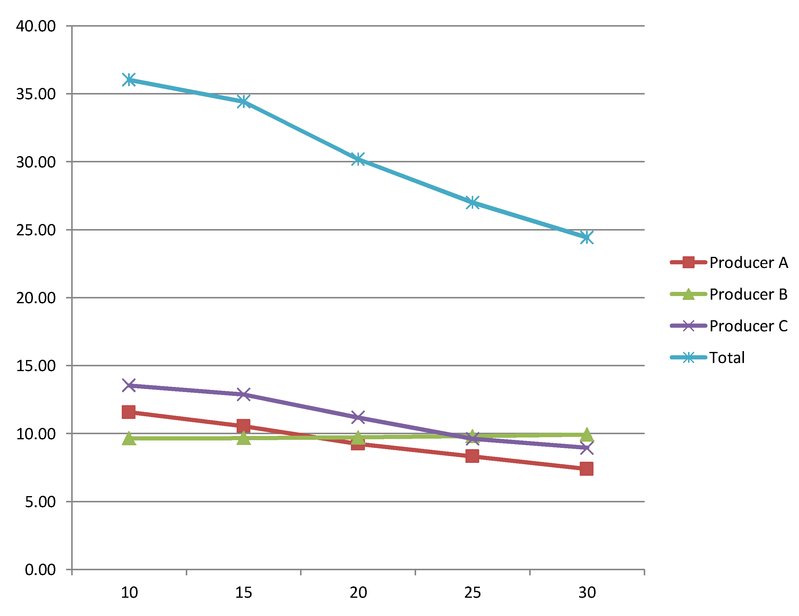
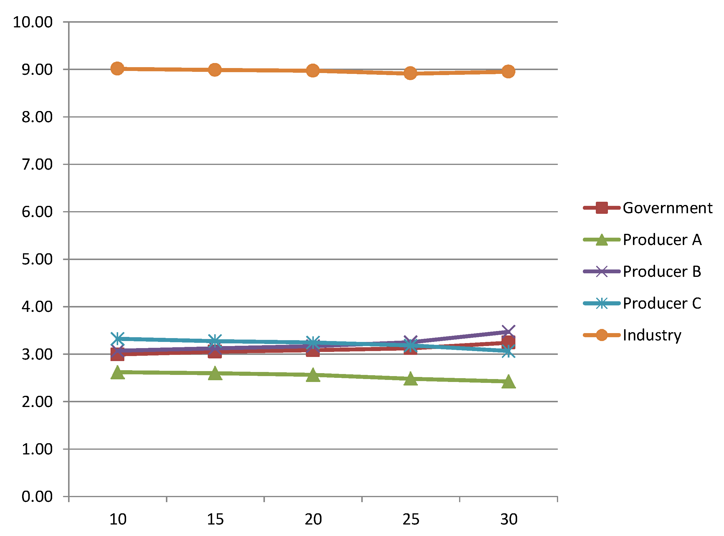
To overcome these difficulties, this paper proposed an integrated methodology for carbon emission reduction problems under an integrated carbon reduction policy. The integrated methodology combined a bi-level mathematical model and an iterative interactive algorithm. The bi-level mathematical model was formulated to handle the leader–followers contradictions and competition between the stakeholders, and FRVs were used to reflect the inherent uncertainties in the problem, all of which made the bi-level mathematical model more complex but better related to the practical environment. An iterative interactive algorithm was designed to solve the non-linear bi-level mathematical model. Then, the proposed methodology was applied to a real-world case, the results from which clearly showed that satisfactory solutions for both the government and the producers could be obtained, and a suitable trade-off reached between economic development and environmental protection. Solution analysis, study of the impact of carbon tax, and comparative analysis in different decision-making environments were conducted to illustrate the applicability and robustness of the proposed methodology.

References

1. Wang, C.; Wang, W.; Huang, R. Supply chain enterprise operations and government carbon tax decisions considering carbon emissions. J. Clean. Prod. 2017, 152, 271–280. [Google Scholar] [CrossRef]
2. Chau, C.K.; Hui, W.K.; Ng, W.Y.; Powell, G. Assessment of CO2 emissions reduction in high-rise concrete office buildings using different material use options. Resour. Conserv. Recycl. 2012, 61, 22–34. [Google Scholar] [CrossRef]
3. Atmaca, A.; Atmaca, N. Life cycle energy and carbon dioxide emissions assessment of two residential buildings in Gaziantep, Turkey. Energy Build. 2015, 102, 417–431. [Google Scholar] [CrossRef]
4. Herrera, J.C.; Chamorro, C.R.; Martín, M.C. Experimental analysis of performance, greenhouse gas emissions and economic parameters for two cooling systems in a public administration building. Energy Build. 2015, 108, 145–155. [Google Scholar] [CrossRef]
5. Shi, Q.; Chen, J.; Shen, L. Driving factors of the changes in the carbon emissions in the Chinese construction industry. J. Clean. Prod. 2017, 166, 615–627. [Google Scholar] [CrossRef]
6. Zhang, X.; Wang, F. Life-cycle assessment and control measures for carbon emissions of typical buildings in China. Build. Environ. 2015, 86, 89–97. [Google Scholar] [CrossRef]
7. Zhang, Z.; Wang, B. Research on the life-cycle CO2 emission of China’s construction sector. Energy Build. 2015, 112, 244–255. [Google Scholar] [CrossRef]
8. Jiang, Z.; Lin, B. China’s energy demand and its characteristics in the industrialization and urbanization process. Energy Policy 2012, 49, 608–615. [Google Scholar] [CrossRef]
9. Dhakal, S. Urban energy use and carbon emissions from cities in China and policy implications. Energy Policy 2009, 37, 4208–4219. [Google Scholar] [CrossRef]
10. Seuring, S.; Müller, M. From a literature review to a conceptual framework for sustainable supply chain management. J. Clean. Prod. 2008, 16, 1699–1710. [Google Scholar] [CrossRef]
11. Porter, M.E.; Van der Linde, C. Green and Competitive: Ending the Stalemate. Harv. Bus. Rev. 1995, 28, 128–129. [Google Scholar]
12. Hollos, D.; Blome, C.; Foerstl, K. Does sustainable supplier co-operation affect performance? Examining implications for the triple bottom line. Int. J. Prod. Res. 2012, 50, 2968–2986. [Google Scholar] [CrossRef]
13. Reid, E.M.; Toffel, M.W. Responding to public and private politics: corporate disclosure of climate change strategies. Strat. Manag. J. 2009, 30, 1157–1178. [Google Scholar] [CrossRef]
14. Bansal, P.; Clelland, I. Talking Trash: Legitimacy, Impression Management, and Unsystematic Risk in the Context of the Natural Environment. Acad. Manag. J. 2004, 47, 93–103. [Google Scholar] [CrossRef]
15. Hajmohammad, S.; Vachon, S. Mitigation, Avoidance, or Acceptance? Managing Supplier Sustainability Risk. J. Supply Chain Manag. 2016, 52, 48–65. [Google Scholar] [CrossRef]
16. Miccoli, S.; Finucci, F.; Murro, R. A monetary measure of inclusive goods: The concept of deliberative appraisal in the context of urban agriculture. Sustainability 2014, 6, 9007–9026. [Google Scholar] [CrossRef]
17. Miccoli, S.; Finucci, F.; Murro, R. Assessing Project Quality: A Multidimensional Approach. Adv. Mater. Res. 2014, 1030, 2519–2522. [Google Scholar] [CrossRef]
18. Miccoli, S.; Finucci, F.; Murro, R. Criteria and Procedures for Regional Environmental Regeneration: A European Strategic Project. Appl. Mech. Mater. 2014, 675, 401–405. [Google Scholar] [CrossRef]
19. Moretti, L.; Caro, S. Critical analysis of the Life Cycle Assessment of the Italian cement industry. J. Clean. Prod. 2017, 152, 198–210. [Google Scholar] [CrossRef]
20. Sorrell, S.; Sijm, J. Carbon trading in the policy mix. Oxf. Rev. Econ. Policy 2003, 19, 420–437. [Google Scholar] [CrossRef]
21. Weisbach, D.A.; Metcalf, G.E. The Design of a Carbon Tax. Soc. Sci. Res. Netw. Electron. J. 2009, 33, 499–556. [Google Scholar] [CrossRef]
22. Carbon Emission Trading. 2017. Available online: https://en.wikipedia.org/wiki/Carbon_emission_trading (accessed on 11 November 2017).
23. Perdan, S.; Azapagic, A. Carbon trading: Current schemes and future developments. Energy Policy 2011, 39, 6040–6054. [Google Scholar] [CrossRef]
24. Intergovernmental Panel on Climate Change. Climate Change 2007 Synthesis Report; Intergovernmental Panel on Climate Change: Geneva, Switzerland, 2007. [Google Scholar]
25. Klemmensen, B.; Pedersen, S.; Rydén, L.; Dirckinck-Holmfeld, K.R.; Marklund, A. Environmental Policy: Legal and Economic Instruments; Baltic University Press: Uppsala, Swdden, 2007. [Google Scholar]
26. Baranzini, A.; Goldemberg, J.; Speck, S. A future for carbon taxes. Ecol. Econ. 2000, 32, 395–412. [Google Scholar] [CrossRef]
27. Fang, G.; Tian, L.; Fu, M.; Sun, M. The impacts of carbon tax on energy intensity and economic growth—A dynamic evolution analysis on the case of China. Appl. Energy 2013, 110, 17–28. [Google Scholar] [CrossRef]
28. Ghosh, D.; Shah, J. A comparative analysis of greening policies across supply chain structures. Int. J. Prod. Econ. 2012, 135, 568–583. [Google Scholar] [CrossRef]
29. Song, J.; Leng, M. Analysis of the Single-Period Problem under Carbon Emissions Policies; Springer: New York, NY, USA, 2012; pp. 297–313. [Google Scholar]
30. Choi, T.M. Carbon footprint tax on fashion supply chain systems. Int. J. Adv. Manuf. Technol. 2013, 68, 835–847. [Google Scholar] [CrossRef]
31. Du, S.; Zhu, L.; Liang, L.; Ma, F. Emission-dependent supply chain and environment-policy-making in the ‘cap-and-trade’ system. Energy Policy 2013, 57, 61–67. [Google Scholar] [CrossRef]
32. Jaber, M.Y.; Glock, C.H.; Saadany, A.M.A.E. Supply chain coordination with emissions reduction incentives. Int. J. Prod. Res. 2013, 51, 69–82. [Google Scholar] [CrossRef]
33. Von Stackelberg, H. The Theory of the Market Economy; Oxford University Press: Oxford, UK, 1952. [Google Scholar]
34. Gibbons, R. Game Theory for Applied Economists; Princeton University Press: Princeton, NJ, USA, 1992. [Google Scholar]
35. Xu, J.; Zhao, S. Noncooperative Game-Based Equilibrium Strategy to Address the Conflict between a Construction Company and Selected Suppliers. J. Constr. Eng. Manag. 2017, 143, 04017051. [Google Scholar] [CrossRef]
36. Xu, J.; Yang, X.; Tao, Z. A tripartite equilibrium for carbon emission allowance allocation in the power-supply industry. Energy Policy 2015, 82, 62–80. [Google Scholar] [CrossRef]
37. Nash, J. Non-cooperative games. Ann. Math. 1951, 54, 286–295. [Google Scholar] [CrossRef]
38. Ben-Ayed, O.; Boyce, D.E.; Iii, C.E.B. A general bilevel linear programming formulation of the network design problem. Transp. Res. Part B 1988, 22, 311–318. [Google Scholar] [CrossRef]
39. Bard, J.F. Practical Bilevel Optimization; Springer: New York, NY, USA, 1998; pp. 144–146. [Google Scholar]
40. Colson, B.; Marcotte, P.; Savard, G. An overview of bilevel optimization. Ann. Oper. Res. 2007, 153, 235–256. [Google Scholar] [CrossRef]
41. Lin, B.; Ouyang, X. Energy demand in China: Comparison of characteristics between the US and China in rapid urbanization stage. Energy Convers. Manag. 2014, 79, 128–139. [Google Scholar] [CrossRef]
42. Hong, J.; Shen, G.Q.; Feng, Y.; Lau, S.T.; Mao, C. Greenhouse gas emissions during the construction phase of a building: A case study in China. J. Clean. Prod. 2015, 103, 249–259. [Google Scholar] [CrossRef]
Figure 1. Model of the bi-level decision-making mechanism in carbon emission reduction.
Sustainability 09 02107 g001
Figure 2. Framework for the iterative interactive algorithm.
Sustainability 09 02107 g002
Figure 3. Influence of different carbon tax values on total carbon emissions (unit: 10 5 t CO 2 ).
Sustainability 09 02107 g003
Figure 4. Influence of different carbon tax values on social benefits and profits (unit: 10 8 CNY ).
Sustainability 09 02107 g004