Article

Policy Uncertainty and the US Ethanol Industry

1
Resource, Energy, and Environmental Economics, RTI International, RTP, NC 27709, USA
2
Department of Agricultural Economics, Texas A&M University, College Station, TX 77840, USA
*
Author to whom correspondence should be addressed.
Sustainability 2017, 9(11), 2056; https://doi.org/10.3390/su9112056
Submission received: 26 September 2017 / Revised: 4 November 2017 / Accepted: 7 November 2017 / Published: 9 November 2017
(This article belongs to the Special Issue Energy Security and Sustainability)

Abstract

:
The Renewable Fuel Standard (RFS2), as implemented, has introduced uncertainty into US ethanol producers and the supporting commodity market. First, the fixed mandate for what is mainly cornstarch-based ethanol has increased feedstock price volatility and exerts a general effect across the agricultural sector. Second, the large discrepancy between the original Energy Independence and Security Act (EISA) intentions and the actual RFS2 implementation for some fuel classes has increased the investment uncertainty facing investors in biofuel production, distribution, and consumption. Here we discuss and analyze the sources of uncertainty and evaluate the effect of potential RFS2 adjustments as they influence these uncertainties. This includes the use of a flexible, production dependent mandate on corn starch ethanol. We find that a flexible mandate on cornstarch ethanol relaxed during drought could significantly reduce commodity price spikes and alleviate the decline of livestock production in cases of feedstock production shortfalls, but it would increase the risk for ethanol investors.

1. Introduction

The Energy Independence and Security Act (EISA) of 2007 mandated 136 billion liters (or 36 billion gallons) of biofuel blending by 2022, including a 56.78 billion liter maximum on conventional ethanol, as well as a 60.56 billion liter minimum on cellulosic ethanol. Ten years after the EISA, the US ethanol industry has experienced significant growth, largely in producing corn-based ethanol, reaching a historical high of 57.77 billion liters by 2016 [1]. However, two major uncertainties evolved with the EISA renewable fuel standard (RFS2) mandate situation. On the cornstarch ethanol side, the mandate has been maintained at a constant level during a given year, even in the face of major shortfalls like the 2012 Midwest drought. This has caused prices to soar in poor production years, increasing price variability in the feedstock market, and has affected parties that compete for the use of those feedstocks, plus those that compete for common resources. EISA allows mandate waivers in RFS2 implementation. A waiver may be issued if (1) the full mandate would “severely harm the economy or environment of a State, a region, or the United States” or (2) “there is an inadequate domestic supply” [1]. The first condition, namely, “economic harm”, is not well defined in the policy and, to date, has not been applied. This research investigates this condition from a corn ethanol perspective.
In relation to the second condition, on the total ethanol side, particularly for cellulosic ethanol, there has been a large discrepancy between the original EISA intentions and the actual implementation of RFS2. For example, EISA originally indicated that about 16 billion liters of cellulosic ethanol would be mandated by 2016, but the final RFS2 mandate was only 0.87 billion liters. This increased the uncertainty faced by those investing in ethanol production and distribution, as they are left unsure as to whether they can sell what they manufacture. The United States Environmental Protection Agency (EPA) has been reducing the EISA cellulosic mandate, citing supply inadequacy for cellulosic ethanol [2] On 28 July 2017, the US Court of Appeals ruled that EPA cannot consider any demand-side constraints when using its waiver authority and remanded the 2016 RFS volume to EPA for further consideration. In the long run, this will not allow EPA to use the ethanol blend wall as a waiver excuse, which is a positive policy signal for the US ethanol industry. This has led to significantly decreased cellulosic mandates, compared with the EISA targets (see Table 1). As argued above, this has lowered ethanol demand and created disincentives for investment in ethanol processing, distribution, and consumption.
In this study, we use both theory and modeling tools to analyze the impact of current and flexible mandates, with the flexibility triggered by production shortfalls. We extend earlier research investigating the short-run impact of an ethanol waiver on crop mix and livestock activity in three main areas. First, by applying a novel use of the decision with the recourse modelling framework described in Section 4.2, we allow for market reaction to drought, while restricting planting and herd size. Secondly, the drought representation in Section 4.1 incorporates spatial, inter-crop, and temporal yield variability, characterizing the realized production impact across the country. Third, we investigate the impacts of several waiver scenarios across differing cellulosic ethanol mandates. Additionally, we investigate the impacts of cellulosic waivers and extend the analysis to include the ethanol producers’ perspectives. We find that increasing the flexibility of ethanol mandates reduces uncertainty for agricultural stakeholders, shifting this uncertainty to the ethanol production sector.

2. Background

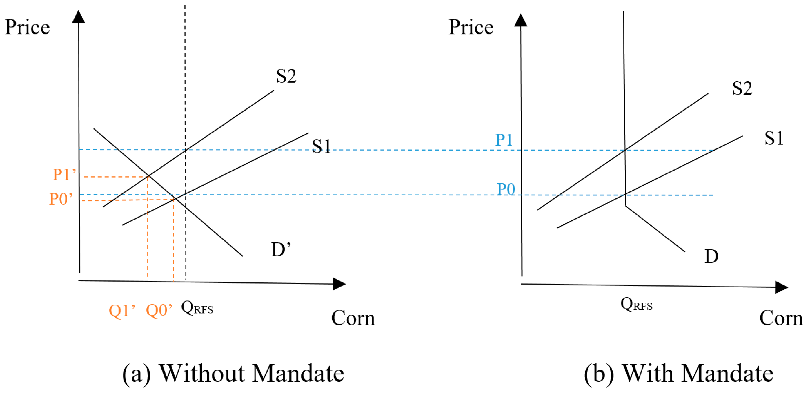
2.1. Uncertainty Caused by a Fixed Mandate in a Fluctuating Feedstock Production

Commodity market effects of fixed RFS2 mandates, given feedstock supply fluctuations, arise in the price of:
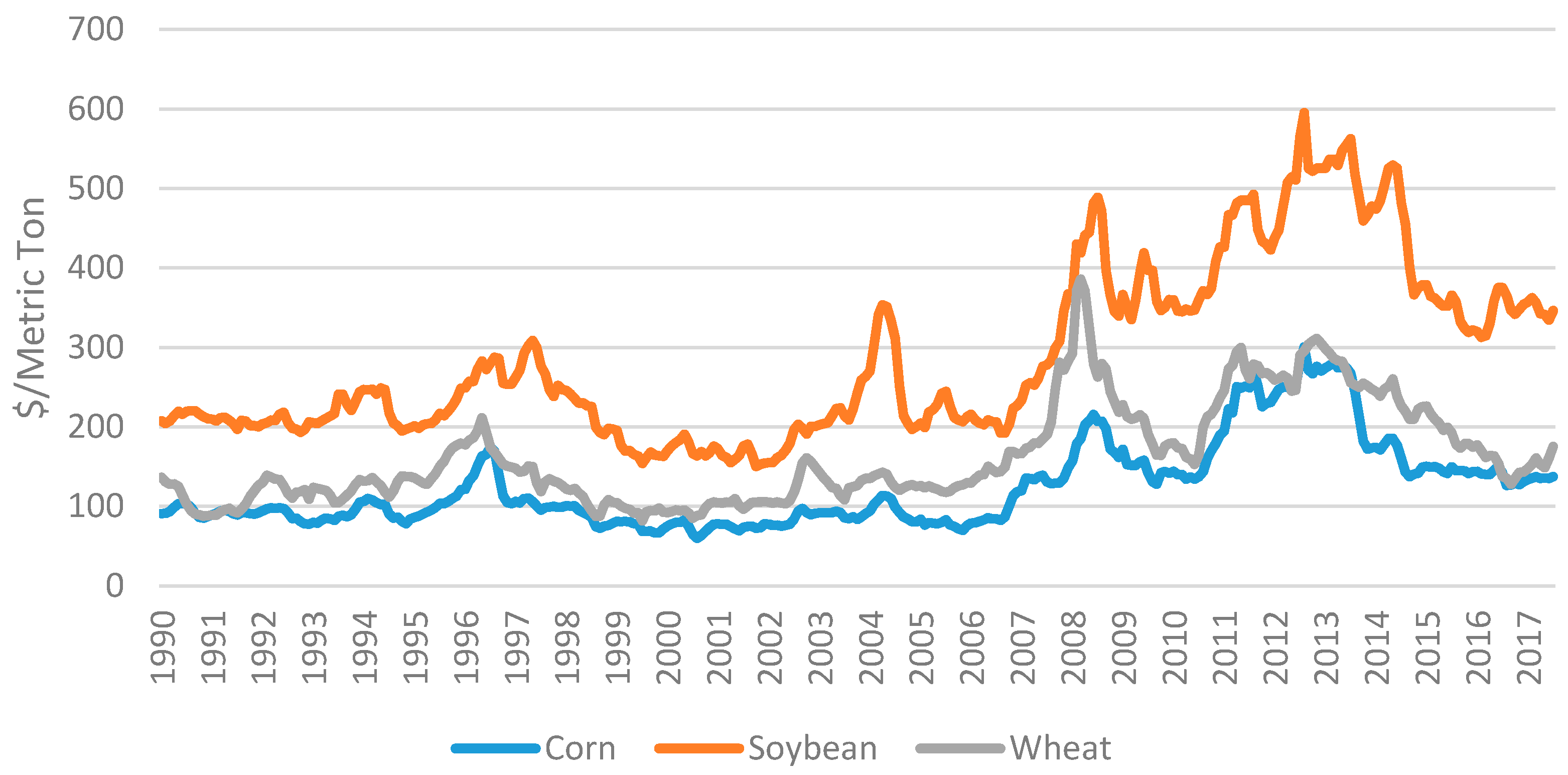
  • Feedstock commodities like corn.
  • Other agricultural commodities that compete for land that could be used for feedstock production.
First, corn has traditionally been an important feed source, a source of export earnings, and an input to some industrial processes. In recent years, it has also become an important biofuel feedstock, with fuel-use demand exceeding feed demand in recent years (using more than 40% of the annual crop). The RFS2 put a fixed mandate on conventional crop biofuel blending with what amounts to a lower and upper bound cap of 56.78 billion liters, using corn as the primary feedstock. This requires that about 127 million metric tons (MT) of corn be used annually for ethanol production [3].
The invariable nature of this mandate can be shown to increase feedstock price variability due to weather and other sources causing fluctuations in supply, which we illustrate using graphical economics in Figure 1. In both panels within Figure 1, we illustrate two supply cases, one with higher production and the other with lower, where S2 is the supply in a low production year and S1 in a higher production year. In panel (a), we have a case with no mandate, and there the supply shock drives the price up from P0’ to P1’ and the production down from Q0’to Q1’. In panel (b) where we have a mandate, it presents ethanol demand at quantities smaller than the mandate. In that case, the price changes from P0 to P1, while the corn used for ethanol production remains unchanged at QRFS. Here, note that the range P0 to P1 is significantly larger than P0’ to P1’, meaning that prices are less stable with the mandate in place. Note this also indicates that significantly less feedstock is available for non-ethanol usages of corn such as livestock feed, dry milling, or exports.
Such a situation does exist in US agriculture. US corn production fluctuates from year to year. It was 312 million metric tons (MT) in 2011, and 351 in 2013, but dropped to 274 million MT in 2012 under the influence of the 2012 drought [4]. However, the mandate was unchanged through all three of these years, at essentially 127 million MT corn, leaving 185, 147, and 224 million MT, respectively, for traditional uses. Thus, feed, export and other non-biofuel demands faced this reduced level of supply in 2012, and the price of corn was pushed to a historical high of $330/MT. This was in comparison to $79 before the RFS2 and $147 today [5]. A more flexible mandate could lower price volatility and contribute to the sustainability of other corn users. An issue is: How much could price volatility be reduced if the mandate is relaxed when supply disruptions occur?
Second, in the case of the broader set of commodities, a similar argument can be made. Consider commodities that compete with corn for land and other inputs. Under the fixed mandate, when yields and total production are low, the mandate yields require more land and other resources to be devoted to corn, leaving less for other uses. This pushes up the price of those commodities and again affects the variability in the marketplace. As shown in Figure 2, we observed positive correlations among the prices of the major crops (i.e., corn, soybeans, and wheat), where biofuel production is one of the contributing factors.
In both cases, a mandate that used lower amounts of feedstock supply under poor conditions would lower market price variability but, on the other hand, would result in less feedstock being available to ethanol producers, less facility utilization, and smaller quantities of fuel being made, raising uncertainty for fuel producers and distributors.

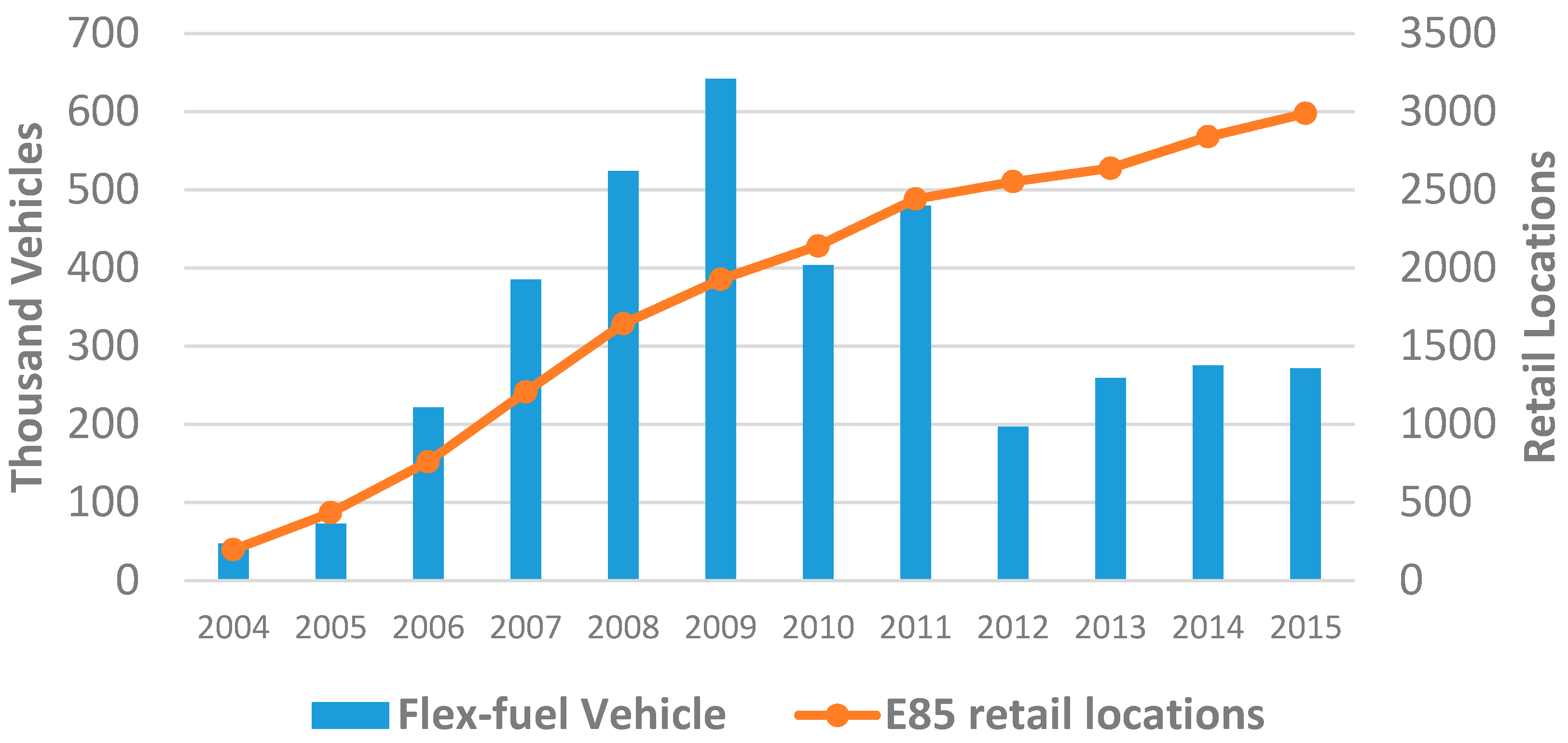
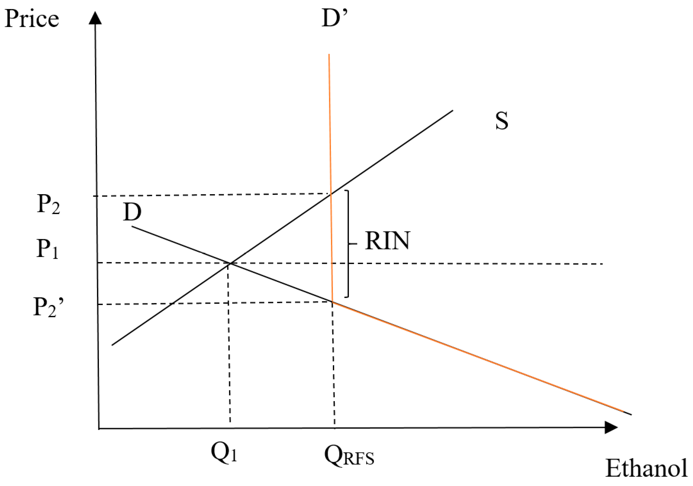
2.2. Uncertainty in Cellulosic Ethanol Production/Distribution Investment

As of today, the state of the US cellulosic ethanol industry is very different from that of the cornstarch ethanol industry. Corn-based ethanol production is well established, with an annual production at the mandated 56.78 billion liter level, but the volume of cellulosic ethanol production is much smaller than that contemplated in EISA. The total 2016 cellulosic ethanol production was 0.67 billion liters [1], in contrast to the original EISA target of 16.09 billion liters. One major reason for this is that cellulosic capability is small and production costs are high, as exhibited by prices for the Renewable Identification Number certificates (RIN). The EPA developed and uses the RIN system under RFS2. This assigns a serial number to each batch of biofuels produced, allows one to track the fuel into blending, and allows obligated parties to prove they complied with the blending mandates. RINS can also be saved into the following year.
McPhail et al. [5] argue that the RIN price is a measure of how much the production cost is above the market price for fuel, plus any transaction costs incurred in the RIN sale. This can be illustrated graphically, as in Figure 3, where S is the ethanol supply and D is the ethanol demand. Additionally, we believe that there is a downward demand curve for ethanol, reflecting the fact that, as volumes increase, it becomes more expensive to use ethanol. This is because investments are needed in infrastructure and vehicles to distribute and consume that ethanol. In the case pictured in Figure 3, the equilibrium price and quantity for the undistorted market condition are given as P1 and Q1, respectively. When a fixed RFS mandate is applied, the demand curve kinks at the mandate, not allowing quantities smaller than QRFS, represented by D’. The new supply price is P2, and the demand price P2’, with the gap between these prices being equal to the RIN price.
The above graphic, coupled with the smaller implemented mandates, lead to two forms of uncertainty for cellulosic ethanol investors (those considering building a new production plant or investing in fuel distribution infrastructure). First, given the higher production cost for cellulosic ethanol production, obtaining the RIN is essential to profitable production. However, only ethanol amounting to the mandate level can receive that RIN. At the same time, the small sizes of the mandate relative to EISA, coupled with the 2017 development that EPA proposed a mandate reduction for 2018 relative to 2017, leaves prospective ethanol production and distribution investors with the question of whether the ethanol product can earn the RFS2 RIN or needs to sell only at the market price. This has manifested itself in a couple of ways. First, the production and development of new ethanol demand by increasing flex fuel vehicles, while initially rapid, has tailed off to very low levels. Second, investment in ethanol production plants has been limited, resulting in low capacity, and, today, no plants are under construction. Third, the incidence of pumps capable of delivering greater than 10% blends is small. Fourth, the limited domestic demand led to exports in recent years. This is a chicken and egg problem; namely, while investment is low, EPA maintains low mandates, and, when mandates are low, investors do not expand capacity.
Finally, there exists feedstock side uncertainty for cellulosic ethanol as well. Most current cellulosic ethanol production is based on agricultural residues such as corn stover, but, like corn, volumes of this are also uncertain, as are yields of other potential feedstocks [6]. Furthermore, while many contemplate dedicated energy crops as a primary feedstock, there is a limited current market for such crops, and they are quite bulky, meaning that the market will largely be a local one. This means that farmers will not grow the dedicated energy crops until plants move in and guaranteed sales contracts are put in place.

3. Literature Review

The effect of biofuel policies on commodity prices has been examined in a number of studies. In this review, we will focus on studies that analyze policies after the introduction of RFS2. Many studies have concluded that the ethanol mandate increased commodity prices [7,8,9]. Condon et al. [8] conducted a meta-analysis and indicated that each additional 3.79 billion-liter (1 billion gallon) expansion in the corn ethanol mandate would lead to a three to four percent increase in 2015 corn prices. Babcock [9] examined the impacts of the 2012 drought and found that the ethanol mandate caused corn prices to increase by more than $39.37/MT (or, one dollar per bushel). However, these analyses did not consider the implications of adjusting the mandate downward when production shortfalls occur.
The literature addressing the impact of RFS2 on commodity price variability is relatively sparse. McPhail and Babcock [10] examined the impacts of RFS2 and the blend wall on corn and gasoline price variability. They indicate that RFS2 creates a floor on ethanol demand, while the blend wall puts on a ceiling. They argue the RFS mandates and the blend wall collectively reduced the corn and gasoline price elasticities of demand and therefore increased price variability. Condon et al. find that the RFS2 also increased the volatility of other commodities [7]. On the other hand, studies have found that RINs could be used to reduce price volatility since they link adjacent years. Namely when corn supply shocks occur, the use of RINs carried over from the previous year can reduce the RFS impact on price volatility [10,11]. Similarly, RINs may be borrowed from a subsequent period by obliged parties. However any negative balances must be made up in the subsequent year. In both cases, this may shift the burden toward next year’s biofuel obligation, influencing future price fluctuations.
Some studies have examined the impact of a flexible mandate on crop markets and livestock [9,12,13,14]. Tyner et al. [12] showed that, to the extent that refiners and blenders used carry-forward RINs, issuing a waiver could benefit livestock producers and consumers but harm ethanol and corn producers. They found that a small waiver would reduce the corn price to around $11.94/kg and that a large waiver would reduce it by as much as $33.02/kg. On the other hand, Good and Irwin argue that a one-year mandate waiver in 2012 would have had a minimal impact on mitigating price volatility [11]. Recently, Hao et al. [15] examined drought impacts on crop, livestock, and biofuel markets, finding that the incentives provided by the waiver might be slow in mitigating the drought’s impact on corn prices.
The effect of cellulosic waivers has also been examined in varying market contexts. Meyer and Thompson [13] find that crop prices, farm income, compliance costs, and greenhouse gas emissions were all sensitive to waiver imposition. Dumortier et al. [16] showed that the exercise of a cellulosic waiver would make landowners unwilling to switch from conventional crops to bioenergy crops, reducing cellulosic feedstock supply. Miao et al. [17] found that a cellulosic waiver had no effect on investment decisions. They also found that, when firm-level marginal costs were not constant, higher RIN prices under a waivable mandate stimulated first stage investment.
Temporal and spatial variation in biomass yield and quality over years and fields may also be a concern, as it affects both ethanol yield and ethanol production. A year-year study of switchgrass production and ethanol yield on 10 switchgrass fields was conducted and analyzed by Schmer et.al [18]. They found that the theoretical mean ethanol yield varied from 1749 to 3691 L ha−1, thus arguing that cellulosic biorefineries should consider imposing an uncertainty discount when developing their business plan. Kim and McCarl show that temporal and spatial aggregation could be used to alleviate this supply side uncertainty [19]. On the demand side, Babcock and Pouliot [20] suggested that the blend wall could be overcome by increasing incentives to use E85. Zhang et al. [21] indicated that relaxing the blend wall could increase the consumption of petroleum gasoline and thus lead to greater energy insecurity.

4. Analytical Approach

To analyze the effects of mandate relaxation, we use a supply demand framework, as presented in an agricultural sector model. Sector modeling is used to examine the price, production, and market impacts of a fixed versus a relaxed corn based ethanol RFS2 mandate. To do this, we incorporate the yield variability into an agricultural sector model and simulate market clearing with and without the relaxed mandate.

4.1. Yield Probability Distribution Formation

Yield variability is an important source of uncertainty in agricultural production. We developed a probability distribution to represent that variability and included it in a stochastic version of the agricultural sector model. Forming the crop yield distribution required the incorporation of both spatial and temporal variability [22], along with the consideration of yield increases due to technology advances. We will estimate an equation for forecasting yields over time and then use the unexplained deviations from that trend to form the yield probability distribution.
In doing this, time dependent regressions were estimated over USDA National Agricultural Statistics Service (NASS) yield data for the major US crops by US state from 1950 to 2012, wherein the advances over time were used as a proxy for technological progress. Also, following Baker et al. [23], we allowed the time advance (technical progress) rate to shift during the time period, possibly slowing down, as has been found in a number of studies [23,24,25]. In turn, the historical deviations from the estimated equations were used to form the probability distributions. Furthermore, we kept the observations together by year, forming correlation relationships between crops and locations.
We also formed a national probability distribution so that we could identify yield shortfall events. In doing this, we took the state level yields for each crop, multiplied by the 2012 acreage planted and summed. The resultant national deviations by year, normalized to the proportion of the mean, are given in Figure 4a. In that figure, note that the 2012 drought exhibits the second largest corn production shortfall since 1950, only exceeded by 1988. The histogram (Figure 4b) exhibits a long left-side tail, accounting for production shortfalls.

4.2. Modeling Approach

An examination of the market impact of yield shortfalls and ethanol waiver policy was done using the stochastic version of the agricultural part of the US Forest and Agricultural Sector Optimization Model (FASOM) [26,27]. This framework maximizes the expected total welfare from US agriculture. The agriculture part of the FASOM model has been widely used to determine the impacts of agricultural, environmental, and biofuel policy on the agricultural sector of the US economy [28]. The model includes such elements as land use, crop and livestock production, commodity processing, greenhouse gas emission considerations, and biofuels, incorporating over 100 commodity types, 40 crops, 25 livestock units, and over 50 processed goods.
The model also represents limited available land, water, labor supply, inputs, import possibilities, alternative tillage, fertilization and irrigation production options, domestic demand, processing demand and byproducts, and export demand. In the sector model, markets clear where the prices are endogenous for factors and products by state of nature.
The stochastic part of the model is based on rational expectation theory. Namely, it assumes that producers do not expect an ethanol waiver but do expect yields to vary and set their crop mix and livestock herd, anticipating that yields will be distributed as in the historical distribution. To implement this, we used a stochastic programming with recourse [29] or a discrete stochastic programming approach [30]. In this case, the model was run using the data behind the above probability distribution, with crop mix and livestock herd size chosen independently of state of nature, and then the market was cleared under each state of nature.

4.3. Analysis design

Mandate relaxation was investigated in several different settings regarding mandate size and relaxation size. Specifically, we ran:
  • Two alternative overall ethanol mandates. We included
    a baseline scenario without ethanol mandates;
    a full EISA mandate scenario with a requirement of 56.78 billion liters for corn based ethanol by 2015, and
  • Mandate relaxation, under which we ran cases with the corn based mandate reduced by half.
The scenarios were run under both normal yields and 2012-like shortfall conditions. Specifically, the 63 years of data collected was grouped into 10 states of nature, as listed in Figure 4b. Year 2012 fell into the black bar (first from left in Figure 4b) together with year 1988, representing a decrease of 18% in production with a probability of two years out of 63.
Moreover, an adjustment was made in the FASOM model structure to depict the impact of potential production shortfalls such as the 2012 drought and potential relaxation in the ethanol mandate. Agricultural producers are not able to predict their occurrence for a given year with complete certainty. Thus, it is assumed in our study that farms make crop mix and livestock breeding herd decisions based on the expected yields at the beginning of the year. However farmers adjust agriculture processing and harvest decisions in case an exogenous short occurs or in the case of potential ethanol mandate relaxation. We first ran the FASOM model with expected yields, then saved the crop mix and livestock breeding herd decisions as ‘lock-in’ levels. Then we ran the model again with the crop mix and livestock herd held at the lock in levels, but we allowed the model to manipulate diets, levels of processing, livestock feeding, and trading patterns.

5. Results

5.1. RFS2 and Corn Ethanol

Table 1 shows the commodity price results that arose under the alternative yield outcomes and RFS mandate cases. In the absence of drought, the projected corn price under 2015 yields was $215.87 per MT. Given that the RFS2 mandate is fully in place, a 2012-like production shortfall in 2015 caused corn prices to nearly double, increasing to $417.89. This increase in corn price is higher than that found in a previous study by Tokgoz et al. [31], which showed that, when conditions like those in the 2012 drought arose under an ethanol mandate scenario, this would cause corn prices to increase by 43.8%. On the other hand, we found that corn prices would only increase by 12% when relaxing the ethanol RFS mandate by 50% under the same drought situation.
Collectively this shows that a RFS waiver would significantly reduce the spike in corn price. The impact of the drought on soybean prices was found to be smaller (i.e., 4% increase). In addition, relaxing the corn ethanol mandates increased soybean prices (i.e., 15%). This is likely due to the biodiesel mandates, a main use of soybeans, as they were not altered and there was a reduced supply of corn oil, pushing soybean oil prices higher. Commodities that are not directly used for energy production (e.g., sorghum, rice, etc.) were also impacted by the RFS mandates, as the price changes are generally higher in the full RFS scenario compared with the prices under the relaxed mandate (Table 2). Finally, the beef price was also impacted due to increasing feeding costs, with the mandate relaxation lowering this effect.
Table 3 summarizes the production and price indices for these scenarios across all crops, where the base case indices were set to 100. Note that the mandate causes all prices to rise by 34.7% relative to the base case, but relaxation reduced this impact to 9.6%. Additionally, the mandate causes all production to decline by about 14%, but mandate relaxation causes production to fall by slightly less (13%). Also, livestock production declined by 8.5% to 9.1% and prices increased by 12% to 13%. Mandate relaxation lowers these effects, with a 2.1% to 2.3% quantity reduction and a 6.4% to 6.8% price increase.

5.1.1. Crop Ethanol Mandate Sensitivity

The results depicted so far were based on a 50% mandate reduction case. We also ran some alternative cases. Table 4 shows the resulting corn price yields under alternative relaxation amounts. Under base yields, corn prices are largely unaffected by moderate mandate decreases. These mandate relaxations under the ample supply case (the 2015 yield projection) have the same effect for any mandate at 49.21 billion liters or less. On the other hand, when a 2012-like production shortfall occurs, the larger the relaxation, the less the increase in corn price (as also found in Condon et al. [8]). Interestingly, our model also showed that, when mandates were removed, corn ethanol production was reduced to levels between 15.52 billion liters under the shortfall and 18.55 under normal yields. This shows that ethanol production would not be zero by RFS elimination but at a level lower than EISA contemplated levels.
Relaxing the mandate increases consumer surplus but decreases producer surplus. Moreover, mandate relaxation also brings uncertainty to ethanol refiners, as discussed in the next section.

5.1.2. Impact on Ethanol Producers

Though shortfall mandate relaxation alleviates pressure on agricultural commodities, it adversely affects ethanol producers in that relaxing the mandate would lead to a decrease in the ethanol plus RIN revenues. Moreover, if the ethanol mandate is relaxed during large shortfalls of corn, and in cases like 2012 and 1988, which occurred in two out of 63 years (about a 3% frequency), the mandate would be relaxed by 50% or by roughly 27 billion liters. Based on the current RIN price of $0.22/liter, the revenue loss would reach $6.25 billion for ethanol producers when such a mandate relaxation is triggered. The expected revenue loss, considering that the mandate is relaxed two years out of 63, is about $0.2 billion, with ethanol producer revenue having a standard deviation of 1.1 billion.

5.2. RFS2 and Cellulosic Ethanol

The previous section dealt with crop ethanol mandates. Here we deal with cellulosic ethanol mandates.

5.2.1. Production Cost and Uncertainty

Currently, cellulosic ethanol is costlier to produce than conventional crop ethanol. As of June 2017, the RIN price for the general ethanol mandate is about $0.22/L, while the RIN price for cellulosic ethanol is $0.70/L. (Data source: Progressive Fuels Limited Weekly Recap at http://www.progressivefuelslimited.com/web_data/PFL_RIN_Recap.pdf, accessed 17 June 2017.) Meanwhile the gasoline and ethanol wholesale prices are $0.41/L (Data source: US Energy Information Administration (EIA) US Total Gasoline Wholesale/Resale Price by Refiners at: https://www.eia.gov/dnav/pet/hist/LeafHandler.ashx?n=PET&s=EMA_EPM0_PWG_NUS_DPG&f=M, accessed 1 November 2017) and $0.42/L (Data source: Official Nebraska Government Website at: http://www.neo.ne.gov/statshtml/66.html, accessed 1 November 2017.), respectively. While the general ethanol wholesale price of $0.41/L already contains the RIN price for corn ethanol [32] and provides good estimators for the corn ethanol production cost (as reflected by P2 in Figure 3), this is not the case for cellulosic ethanol, as its RIN price is higher than the wholesale ethanol price. An alternative approximation for the cellulosic ethanol cost is the wholesale gasoline price (adjusted by the energy content difference) plus the RIN price, leading to $0.97/L. For this, we used the following equation, as suggested by Dr. Wallace E Tyner: A p p r o x i m a t e d   C e l l u l o s i c   e t h a n o l   p r i c e = W h o l e s a l e   g a s o l i n e   p r i c e   2 / 3   +   C e l l u l o s i c   e t h a n o l   R I N   p r i c e
Estimates from the literature and industry also indicate a much higher cellulosic ethanol cost than the ethanol market price. The US Department of Agriculture estimated that production cost was $0.70/L [33]. Estimates from the National Renewable Energy Laboratory [34] placed the production cost of cellulosic ethanol at $0.57/L, based on a pilot plant study. A recent study by Johnson [35] assessed the production cost of cellulosic ethanol with an integrated enzyme production method to be $0.62 to $0.73 per liter. A detailed review of recent technological progress is available by Kumar et al. [36]. On the industry side, a report from POET LLC indicated that their 2009 cost was $0.62/L [37]. A 2012 survey conducted by Bloomberg New Energy Finance found that the cost was $0.94/L. A January 2017 report by Lux Research assessed the production cost across six operating facilities and found a range from $0.57 to $1.20 per liter.
The cost estimates and market/RIN price sum shows cellulosic ethanol to be not economically competitive at the existing market price. Thus, the RIN associated with mandate satisfaction is crucial for ethanol producers, creates incentives for investment, and has so far stimulated the growth of cellulosic ethanol industry [38]. However, the EPA has been greatly reducing the RFS2 cellulosic mandates relative to the levels contemplated in EISA. Moreover, the EPA has allowed renewable natural gas generated from sources such as landfills and agricultural digesters to receive RINs and count as cellulosic ethanol in fulfilling the RFS obligation [39]. They also tried in the Summer of 2017 to reduce the volume requirement relative to previous years. This both has reduced the market size of the cellulosic RIN market and portends even further reduction. Certainly, this creates concerns for possible investors as to whether the higher and costly volumes of ethanol they might produce will be able to make up the difference between production costs and market sales using RINs.
Thus, production capability is small; as of 12 May 2017, there are seven operating cellulosic plants, with a total capacity slightly above 0.19 billion liters, plus eight proposed plants, adding another 0.7 billion-liter capacity, with none under construction. (Data from ethanolproducer.com at http://www.ethanolproducer.com/plants/listplants/US/Proposed/Cellulosic, accessed 19 June 2017).

5.2.2. Feedstock Uncertainty

Another uncertainty source regarding cellulosic production involves yield uncertainty and small markets. Generally, a cellulosic plant will wish to operate regardless of yield shortfalls. It is likely that the plant will need to contract for more than the needed amount of feedstock to have enough to keep the plant fully stocked even under yield shortfalls. Plants can alleviate feedstock uncertainty by contracting for enough land area, not based on an average amount but rather on the average minus an uncertainty discount. This, following Kim and McCarl [19], is the mean times a factor is equal to 1 z α · C V , where CV is the coefficient of variation for feedstock yield, z is score nominally from a normal distribution table, and α is the probability coefficient. Schmer et al. [18] estimated the CV for switchgrass yield, ranging from 0.14 to 0.38. Thus, using z α = 1.64, which implies a 95% confidence level with a single-tail, the uncertainty discount factor would range from 0.38 to 0.77. To put this into context, adapting assumptions from the 2015 Billion-Ton report [40], a 40-million-liter-year ethanol biorefinery might need roughly 12 thousand hectares of switchgrass land based on the average yield (8.15 dry tons per hectare at a conversion rate of 400 liters per dry ton). However, the required area could go up to 15.58 to 31.58 thousand hectares to provide this safety buffer. Furthermore, this would still have a five percent chance of falling short and would generally result in more switchgrass being available than needed, introducing the need for year to year storage, use in some other market by, say, pelleting and shipping, and/or disposal. This could also raise the amount of land that needs to be contracted and thus the ethanol production cost.
The feedstock uncertainty discount can be reduced through spatial diversification or year to year storage. For example, Kim and McCarl [19] show by using corn variation that the CV can be reduced from 32.39% to 9.78% when feedstock is assembled broadly across a county or crop reporting district as opposed to a single location. Additionally, they show that the CV over five years falls to 1.58%, meaning that storage from year to year would create a much more certain supply, but this, again, would raise costs.

5.3. Demand Uncertainty

Ethanol is not a perfect substitute for gasoline, which is mainly due to infrastructure incompatibility. As a result, the maximum percentage of ethanol allowed to be blended into gasoline is 15% (known as E15) with the existing infrastructure and vehicles [41]. In fact, most gasoline consumed in the US is blended with only 10% ethanol (E10). Since the annual consumption of gasoline in US is around 530 billion liters, the maximum domestic ethanol consumption would be stuck at 53 billion gallons. In fact, the US has been an ethanol exporter since 2010, when ethanol production surpassed 10% of the domestic quantity of gasoline consumed (the apparent blend wall limit imposed by distribution and demand considerations) [42].
To achieve higher ethanol market penetration (commonly E85), investments in infrastructure (i.e., new fuel distribution pumps, storage, and pipelines) and flex-fuel cars are needed. However, such investment has only occurred at a very low level. As shown in Figure 5, the inventory of Flex-fuel vehicles in the US that are eligible for higher ethanol levels (E85) has been constant for the past few years, with new models not being introduced. Meanwhile, the number of gas stations with the E85 option was slightly above 3000 by end of 2015, and the majority of them were located in Corn Belt states, where most ethanol was produced. To put this into context, there are about 156,000 gas stations nationwide, thus gas station with the E85 option constitute about 2%.
In sum, the previous mandate situation on cellulosic ethanol has caused investors to be uncertain as to the extent of the amount of fuel they could sell under future mandates or in the future market plus a regulatory environment (i.e., price supports through RINS) that covers cost. As a result, investment in cellulosic biorefinery production facilities, and even research and development, has been stagnant, or, in cases, ceased, for the past few years. Moreover, cellulosic feedstock supply could also suffer from production shortfalls similar to the discussion of corn ethanol, bringing further uncertainty to cellulosic ethanol development. Thus it is expected that the future development of the cellulosic industry will require policy support.

6. Conclusions and Discussion

Bioenergy production from agriculture involves several major risks. This research focused on the risks faced by a certain subset of bioenergy stakeholders. However it is important to note that other sources of economic and environmental risks also exist. The risk discussed in this analysis arises from yields and government policy. Furthermore, the management of risks has different effects on crop producers, livestock producers, consumers, and ethanol producers. Actions like mandate relaxation reduce the risk faced by consumers and livestock producers but increase those to crop producers and ethanol processers. Rigidities in the short-run ethanol demand curve due to plant reconfiguration and octane requirements were not considered in this analysis [43]. Future analyses should incorporate the techno-economic considerations of process timing, plant size, logistical considerations, and non-yield associated risks when formulating both the demand and supply of ethanol. Another important part of this problem, particularly when the timeframe is extended, is the role of international trade. Although the short-run trade response may be limited, long run analyses should consider global impacts when considering large changes in US ethanol policy.
Reducing long run mandates increases processor risk and reduces production. Adding a yield discount when contracting for feedstock raises cost and reduces the incidence of shortfall but increases the need to dispose items when yield surpluses occur. Widening the spatial basis for contracting decreases risk. The result of these uncertainties has been lower levels of investment in cellulosic ethanol production capacity and overall distribution capability. Increasing investment will likely require higher mandates or other forms of policy support.

Author Contributions

Jason P. H. Jones and Bruce A. McCarl conceived and designed the experiments and Jason P.H. Jones and Zidong Wang performed the experiments. The paper was written by all.

Conflicts of Interest

The authors declare no conflict of interest.

References

  1. Renewable Fuels Association. Annual Ethanol Industry Outlook 2017. Available online: http://www.ethanolrfa.org/resources/publications/outlook/ (accessed on 21 September 2017).
  2. Bracmort, K. The Renewable Fuel Standard (RFS): Cellulosic Biofuels. Congr. Res. Serv. 2015, 31, 1–21. [Google Scholar]
  3. USDA; Commodity Forecasts. World Agricultural Supply and Demand Estimates. Available online: https://www.usda.gov/oce/commodity/wasde/ (accessed on 28 June 2017).
  4. USDA National Agricultural Statistics Service Quick Stats—Corn Condition. Available online: https://quickstats.nass.usda.gov/ (accessed on 27 June 2017).
  5. USDA ERS Feed Grains Custom Query. Available online: https://data.ers.usda.gov/FEED-GRAINS-custom-query.aspx (accessed on 28 June 2017).
  6. Carriquiry, M.A.; Du, X.; Timilsina, G.R. Second generation biofuels: Economics and policies. Energy Policy 2011, 39, 4222–4234. [Google Scholar] [CrossRef]
  7. Taheripour, F.; Tyner, W.E. Welfare Assessment of the Renewable Fuel Standard: Economic Efficiency, Rebound Effect, and Policy Interactions in a General Equilibrium Framework. In Modeling, Dynamics, Optimization and Bioeconomics I; Springer Proceedings in Mathematics & Statistics; Springer: Cham, Switzerland, 2014; pp. 613–632. ISBN 978-3-319-04848-2. [Google Scholar]
  8. Condon, N.; Klemick, H.; Wolverton, A. Impacts of ethanol policy on corn prices: A review and meta-analysis of recent evidence. Food Policy 2015, 51, 63–73. [Google Scholar] [CrossRef]
  9. Babcock, B.A. Preliminary Assessment of the Drought’s Impacts on Crop Prices and Biofuel Production; CARD Policy Brief 12-PB; Iowa State University: Ames, IA, USA, 2012. [Google Scholar]
  10. McPhail, L.L.; Babcock, B.A. Impact of US biofuel policy on US corn and gasoline price variability. Energy 2012, 37, 505–513. [Google Scholar] [CrossRef]
  11. Good, D.; Irwin, S. Ethanol—Does the RFS Matter; Farmdoc Daily; University of Illinois at Urbana-Champaign: Champaign, IL, USA, 2012. [Google Scholar]
  12. Tyner, W.E.; Taheripour, F.; Hurt, C. Potential Impacts of a Partial Waiver of the Ethanol Blending Rules. 2012. Available online: https://www.semanticscholar.org/paper/Potential-Impacts-of-a-Partial-Waiver-of-the-Ethan-Akridge-Conklin/52cd92316b53e4f847cd0883569e311f96809e19 (accessed on 28 June 2017).
  13. Meyer, S.; Thompson, W. How Do Biofuel Use Mandates Cause Uncertainty? United States Environmental Protection Agency Cellulosic Waiver Options. Appl. Econ. Perspect. Policy 2012, 34, 570–586. [Google Scholar] [CrossRef]
  14. Tejeda, H.A. Time-Varying Price Interactions and Risk Management in Livestock Feed Markets—Determining the Ethanol Surge Effect. Available online: https://www.researchgate.net/publication/254384312_Time-Varying_Price_Interactions_and_Risk_Management_in_Livestock_Feed_Markets_-_Determining_the_Ethanol_Surge_Effect (accessed on 12 June 2017).
  15. Hao, N.; Colson, G.; Seong, B.; Park, C.; Wetzstein, M. Drought, ethanol, and livestock. Energy Econ. 2015, 49, 301–307. [Google Scholar] [CrossRef]
  16. Dumortier, J.; Kauffman, N.; Hayes, D.J. Uncertainty and Time-to-Build in Bioenergy Crop Production. In Proceedings of the AAEA & WAEA Joint Annual Meeting, San Francisco, CA, USA, 26–28 July 2015. [Google Scholar]
  17. Miao, R.; Hennessy, D.A.; Babcock, B.A. Investment in Cellulosic Biofuel Refineries: Do Waivable Biofuel Mandates Matter? Am. J. Agric. Econ. 2012, 94, 750–762. [Google Scholar] [CrossRef]
  18. Schmer, M.R.; Vogel, K.P.; Mitchell, R.B.; Dien, B.S.; Jung, H.G.; Casler, M.D. Temporal and spatial variation in switchgrass biomass composition and theoretical ethanol yield. Agron. J. 2012, 104, 54–64. [Google Scholar] [CrossRef]
  19. Kim, M.-K.; McCarl, B.A. Uncertainty discounting for land-based carbon sequestration. J. Agric. Appl. Econ. 2009, 41, 1–11. [Google Scholar] [CrossRef]
  20. Babcock, B.A.; Pouliot, S. Price It and They Will Buy: How E85 Can Break the Blend Wall. 2013. Available online: http://www.card.iastate.edu/products/publications/synopsis/?p=1187 (accessed on 28 June 2017).
  21. Zhang, Z.; Lohr, L.; Escalante, C.; Wetzstein, M. Food versus fuel: What do prices tell us? Energy Policy 2010, 38, 445–451. [Google Scholar] [CrossRef]
  22. Hammer, G.L.; Hansen, J.W.; Phillips, J.G.; Mjelde, J.W.; Hill, H.; Love, A.; Potgieter, A. Advances in application of climate prediction in agriculture. Agric. Syst. 2001, 70, 515–553. [Google Scholar] [CrossRef]
  23. Baker, J.S.; Murray, B.C.; McCarl, B.A.; Feng, S.J.; Johansson, R. Implications of Alternative Agricultural Productivity Growth Assumptions on Land Management, Greenhouse Gas Emissions, and Mitigation Potential. Am. J. Agric. Econ. 2013, 95, 435–441. [Google Scholar] [CrossRef]
  24. Villavicencio, X.; McCarl, B.A.; Wu, X.M.; Huffman, W.E. Climate change influences on agricultural research productivity. Clim. Chang. 2013, 119, 815–824. [Google Scholar] [CrossRef]
  25. Beddow, J.M.; Pardey, P.G.; Alston, J.M. The Shifting Global Patterns of Agricultural Productivity. Available online: http://www.choicesmagazine.org/UserFiles/file/article_95.pdf (accessed on 7 November 2017).
  26. Adams, D.M.; Alig, R.J.; McCarl, B.A.; Murray, B.C. FASOMGHG Conceptual Structure, and Specification: Documentation. Available online: http://agecon2.tamu.edu/people/faculty/mccarl-bruce/papers/1212FASOMGHG_doc.pdf (accessed on 7 November 2017).
  27. Beach, R.H.; McCarl, B.A. US Agricultural and Forestry Impacts of the Energy Independence and Security Act: FASOM Results and Model Description. Available online: https://yosemite.epa.gov/sab/SABPRODUCT.nsf/962FFB6750050099852577820072DFDE/$File/FASOM+Report_EISA_FR.pdf (accessed on 8 July 2017).
  28. Schneider, U.A.; McCarl, B.A. Implications of a Carbon Based Energy Tax for US Agriculture. Agric. Resour. Econ. Rev. 2005, 34, 265–279. [Google Scholar] [CrossRef]
  29. Dantzig, G.B. Linear programming under uncertainty. Manag. Sci. 1955, 1, 197–206. [Google Scholar] [CrossRef]
  30. Cocks, K.D. Discrete stochastic programming. Manag. Sci. 1968, 15, 72–79. [Google Scholar] [CrossRef]
  31. Tokgoz, S.; Elobeid, A.; Fabiosa, J.; Hayes, D.J.; Babcock, B.A.; Yu, T.H.E.; Dong, F.; Hart, C.E. Bottlenecks, drought, and oil price spikes: Impact on US ethanol and agricultural sectors. Appl. Econ. Perspect. Policy 2008, 30, 604–622. [Google Scholar] [CrossRef]
  32. Knittel, C.R.; Meiselman, B.S.; Stock, J.H. The Pass-through of RIN Prices to Wholesale and Retail Fuels under the Renewable Fuel Standard; National Bureau of Economic Research: Cambridge, MA, USA, 2015. [Google Scholar]
  33. Collins, K. The new world of biofuels: Implications for agriculture and energy. In Proceedings of the EIA Energy Outlook, Modelling and Data Conference, Washington, DC, USA, 2007; Available online: www.pitt.edu/~super4/36011-37001/36841.ppt (accessed on 21 July 2017).
  34. Bratis, A. NREL Cellulosic Ethanol Cost Target 2012. Available online: https://energy.gov/sites/prod/files/2016/05/f31/day_two_plenary_cellulosic%20cost%20target_bratis.pdf (accessed on 21 September 2017).
  35. Johnson, E. Integrated enzyme production lowers the cost of cellulosic ethanol. Biofuels Bioprod. Bioref. 2016, 10, 164–174. [Google Scholar] [CrossRef]
  36. Kumar, R.; Tabatabaei, M.; Karimi, K.; Sárvári Horváth, I. Recent updates on lignocellulosic biomass derived ethanol-A review. Biofuel Res. J. 2016, 3, 347–356. [Google Scholar] [CrossRef]
  37. Coyle, W.T. Next-Generation Biofuels: Near-Term Challenges and Implications for Agriculture; DIANE Publishing: Collingdale, PA, USA, 2010. [Google Scholar]
  38. Schnepf, R.; Yacobucci, B.D. Renewable Fuel Standard (RFS): Overview and Issues. Available online: https://www.ifdaonline.org/IFDA/media/IFDA/GR/CRS-RFS-Overview-Issues.pdf (accessed 7 November 2017).
  39. United States Environmental Protection Agency. Renewable Fuel Pathways II Final Rule to Identify Additional Fuel Pathways under Renewable Fuel Standard Program. Available online: https://www.epa.gov/renewable-fuel-standard-program/renewable-fuel-pathways-ii-final-rule-identify-additional-fuel (accessed on 19 June 2017).
  40. Langholtz, M.H.; Stokes, B.J.; Eaton, L.M. 2016 Billion-Ton Report: Advancing Domestic Resources for a Thriving Bioeconomy; Oak Ridge National Laboratory: Oak Ridge, TN, USA, 2016.
  41. Szulczyk, K.B. Which is a better transportation fuel-butanol or ethanol? Int. J. Energy Environ. 2010, 1, 501–512. [Google Scholar]
  42. Tyner, W.E. Policy Update: The US Renewable Fuel Standard up against the Wall; Taylor & Francis: Abingdon, UK, 2013. [Google Scholar]
  43. US EPA. Notice of Decision Regarding Requests for a Waiver of the Renewable Fuel Standard. Federal Register Vol. 77, No. 228. Available online: https://www.gpo.gov/fdsys/pkg/FR-2012-11-27/pdf/2012-28586.pdf (accessed on 19 September 2017).
Figure 1. Illustrative change in corn price and quantity used with (b) and without (a) mandate.
Sustainability 09 02056 g001
Figure 2. Monthly price received for corn, soybean, and wheat from 1990 to 2017 Data source: United States Department of Agriculture, National Agricultural Statistics Service at https://www.nass.usda.gov/Charts_and_Maps/Agricultural_Prices/. Accessed 1 September 2017.
Sustainability 09 02056 g002
Figure 3. RFS2 mandate and price impact.
Sustainability 09 02056 g003
Figure 4. Corn production deviation using normalized 2012 acres (a) and the resulting distribution (b).
Sustainability 09 02056 g004
Figure 5. Flex-fuel Vehicle Inventory and E85 retail locations from 2004 to 2015. Data from Alternative Fuels Data Center at https://www.afdc.energy.gov/data/10581 and https://www.afdc.energy.gov/data/10354. Accessed 20 June 2017.
Sustainability 09 02056 g005
Table 1. Energy Independence and Security Act (EISA) cellulosic target versus final renewable fuel standard (RFS2) rule by year. Source: Final RFS2 rules from EPA websites available from https://www.epa.gov/renewable-fuel-standard-program/regulations-and-volume-standards-renewable-fuel-standards. Accessed 16 June 2017.
EISA TargetEPA Final Rule
20100.380.02
20110.950.02
20121.890.04
20133.790.00
20146.620.06
201511.360.47
201616.090.87
201720.821.18
201826.500.90 (proposed)
201932.18
202039.75
202151.10
202260.57
Note: EISA target is in billion liters, and EPA final rule is in billion ethanol-equivalent liters.
Table 2. Corn and Soybean Price Results for 2015 under a 2012-like Supply Reduction.
Price ($/MT)Full RFS2, Normal YieldEffects of 2012 Production Short-Fall Scenarios
Full RFS2 and Short-Fall%Δ from BaseRelaxed
RFS2 by 50%
and Short-Fall
%Δ from Base
Corn$215.87$417.8994%$242.3512%
Soybeans$413.95$429.104%$477.7815%
Wheat$245.49$374.4952%$251.302%
Sorghum$208.92$402.0792%$234.2412%
Rice$307.72$372.7821%$306.920%
Oats$278.10$363.3231%$318.8415%
Barley$236.85$334.0241%$237.220%
Fed Beef *$10.89$11.899%11.445%
Note: *: Fed beef price is in $ per kg.
Table 3. Crop Production and Price Indices Following the 2012 Drought.
Price IndexProduction Index
Full RFSRFS Relaxed 50%Full RFS2RFS2 Relaxed 50%
134.7109.685.986.7
Table 4. 2015 Corn Price in $/MT Sensitivity to Crop Ethanol Mandates, Given the 2012 Drought
Crop Ethanol Mandate in Billion Liters
(Billion Gallons in Parentheses)
Normal Yields2012 Drought Regression Scenario
Full RFS2 (15)$215.87$417.89
53.00 (14)$206.82$388.15
49.21 (13)$204.56$369.83
45.42 (12)$204.56$351.11
41.63 (11)$204.56$336.72
37.85 (10)$204.56$314.07
34.07 (9)$204.56$297.71
30.28 (8)$204.56$285.69
26.50 (7)$204.56$276.03
Baseline (0)$204.56$242.35

