Mobility of Workers and Population between Old and New Capital Cities Using the Interregional Economic Model

Abstract

The purpose of this paper is to analyze the effects of transportation and mobility costs on the mobility of workers and the overall population between old and new capital cities. First of all, mobility costs clearly have a negative effect on utility; higher commuting costs could lead to the spatial dispersion of workers. In addition, if the monthly commuting cost exceeds 1290 USD between Seoul (the old capital) and Sejong (the new capital), it would be efficient for workers in Seoul to move to Sejong. Finally, the interregional population equilibrium could be achieved when the share of transportation cost to commodity price reaches 60.1%.

1. Introduction

Economic concentration in Seoul, the capital city of Korea, has had a negative impact on urban sustainable growth, interregional balanced development, the housing market, and environmental pollution [1]. To tackle this issue with policy tools, the Korean government decided to relocate 36 government ministries and agencies from Seoul to Sejong city (approximately 160 km south of Seoul, the capital city of Korea), the new administrative capital, in 2007, with the Presidential Office, the National Assembly, and all the foreign embassies remaining in Seoul. This location policy is not new for Asian countries. Malaysia constructed a new administrative capital, Putrajaya, in the early 1990s, and has transferred the federal administrative offices to this capital. Indonesia and Japan have discussed the construction of new administrative capital cities since the 1980s.

The success of this relocation as a strong population dispersion tool depends on the outflows of government officers and families from Seoul and subsequent relocations of major commercial and financial facilities. For example, the planned population size of Putrajaya in Malaysia is 340,000 by 2025, but the actual size as of 2015 is only 83,000. Sejong City aims to grow into a sustainable self-sufficient city with a population of 500,000 by 2030, but the population size remains at roughly 40% of the population goal. What are the practical policy options for the government to achieve this planning target? In the sense that spatial economic activities have been assessed in terms of transportation costs and agglomeration economy, this paper is concerned with the economic contribution of transportation and mobility costs to the migration between the old and the new capital cities.

The purpose of this paper is to analyze the effects of transportation costs on the mobility of workers and the general population between the old and new capital cities using a two-region growth model. Previous studies have analyzed a spatial framework between two regions, in each of which workers can reside or work. They divided mobility on the interregional level into commuting and migration depending on relocation decisions between two regions [2,3,4]. This paper attempts to examine the impacts of transportation and mobility costs on consumers’ utility and the spatial distribution of workers. Transportation cost is logistically defined as the shipping (trade) cost of commodities, whereas mobility costs are the costs of commuting and migration of workers [3]. In addition, the financial subsidies to move workers from the old capital to the new capital are derived from the comparative analysis of the theoretical model. The paper proceeds as follows: Section 2 presents a literature review on the effect of transportation costs and migration; Section 3 develops a simple two-region model; Section 4 explores the comparative analysis; Section 5 performs a numerical simulation with the use of transportation and commuting costs; and Section 6 summarizes this paper and discusses further research issues.

2. Literature Review

2.1. Effects of Transportation and Mobility Costs

Traditionally, in spatial economics, some literature has focused on the commute of workers on the intraregional level, but other literature has studied relocation decisions on the interregional level with respect to transportation and mobility costs. Transportation and mobility costs are traditionally key factors that affect the relocation of economic activities such as commuting or migration. Here, we present some examples of the effect of transportation costs on economic activities. Lower transportation costs, economies of scale, product differentiation, and positive general equilibrium feedback apparently work against the development of remote and sparsely populated suburb areas [5]. Kilkenny (1998) reviewed the relationship between transportation cost, mobility, and the rural development of firms and workers. Changes in transportation costs affected regional wage rates, thus determining the location of production cost-oriented firms and affecting the spatial mobility of firms and workers. A reduced transportation cost could result in the optimal number of firms and the concentration of firms in each region [6]. Tabuchi et al. (2005) analyzed the effects of a decrease in intercity transportation cost on the spatial distribution of the population in multiregional economies. The decrease in transportation cost triggered an agglomeration process in which large cities attracted workers and firms from the small cities [7]. However, Tabuchi (1998) demonstrated that when the transportation cost was low enough to overcome the advantages of agglomeration, dispersion prevailed under equilibrium within a two-region framework [8]. Murata and Thisse (2005) examined how low transportation cost facilitated the dispersion of economic activities within a general equilibrium model [9]. Alstadt et al. (2012) analyzed the relationship between transportation access, connectivity and local economic outcomes within an industry. The local 40-min and the regional three-hour market sizes in the trade and service industrial sectors were consistently strong factors that affected industry employment concentration, industry labor productivity, and foreign export proportion. However, these factors were less strong in the manufacturing, construction, and industrial utility sectors [10]. Allio (2016) found that if trade costs are low, the firms of each region access almost the same market wherever they settle, and workers consume products indifferently from the two regions. Thus, when trade costs increase, the agglomeration forces overpass the dispersion [11].

From the analysis of mobility costs, Suh (1988) defined conditions where intercity commuting was plausible. Workers lived in two strip cities that differed in terms of distance from the center, average rental prices, and commuting cost, with the absence of migration cost. When the income gap was large enough relative to the distance between the two cities and to the commuting cost, the residents of the low-income city tended to commute for work to the high-income city, despite the commuting cost [12]. Pinto (2002) observed that a reduction in commuting cost could lead to mobility [2]. Murata and Thisse (2005) assumed that workers could be mobile and free to choose a region where they preferred to work and live. They showed that a high commuting cost fostered economic activities [9]. Anas et al. (1998) and Anas and Rhee (2007) indicated that toll fees, as a commuting cost, reduced inefficient suburb-to-city commuting, as demonstrated in a simple city–suburb model with cross-commuting [13,14]. Baum-Snow (2007a; 2007b) found that in metropolitan areas where the intra-highway system was more developed, the population would be less concentrated at the center of the metropolitan city. Therefore, the degree of suburbanization was higher [15,16]. Using a two-city model, Sorek (2009) showed how workers’ migration or commuting decisions depended on commuting or migration cost and on commuting time. The migrants were the most able workers of the suburb. Suburb workers exhibited moderate ability to commute to work in the metropolis, and became the least able workers in suburbs. This showed that a reduction in commuting time could moderate, stop, or reverse the migration process. Potential intercity commuting time sharply declined with the development of transport technology. Therefore, commuting beyond the monocentric framework or between distant cities where workers could reside and work is made possible [3]. Xu and Li (2016) stressed the relation between commuting time and dispersion or agglomeration. They revealed that, from the empirical evidence, service employment decreased by 7%, but manufacturing employment increased by 21% in noncore areas in Japan [17].

In short, reducing intercity transportation costs could induce the concentration or dispersion of production factors. Higher commuting cost mostly resulted in population dispersion in a multiregional economy. The lower commuting time caused by the development of transportation technologies could result in population dispersion to suburban areas.

2.2. Migration

Market-driven factors and public sector programs induce migration. For market-driven factors, Todaro (1969) and Harris and Todaro (1970) emphasized that a relatively higher permanent income or urban–rural differences in expected earnings attracted a steady stream of rural migrants into urban areas based on the market mechanism [18,19]. Cristopher and McMaster (1990) concluded that the market mechanism could remove regional inequality in economic prosperity. Interregional migration was found to respond to changes in regional wages and differences in employment opportunities. Migration induced by changes in unemployment rates restored the system to equilibrium [20]. Cushing and Poot (2004) stressed that migration was a result of a forward-looking behavior to maximize an individual’s or a household’s expected future benefit against cost [21]. Kancs (2011) studied the determinants of migration, such as market potential, wages, and cost of living in European regions [22].

For a public sector program, Tiebout (1956) suggested that an increase in consumer voter knowledge could improve the allocation of government expenditures [23]. Porell (1982) examined the effect of economic incentives and quality of life factors such as climate, parks, sports events, crime, density, and public welfare payments [24]. Cristopher and McMaster (1990) determined the necessity of a regional policy that could move jobs to a depressed region to eliminate the disequilibrium of the unemployment differential. In addition, mobility in acquiring jobs and knowledge relevant to the location of the industry and workers could improve the allocation of private resources [20]. Marshall et al. (2005) estimated the positive effects of public sector dispersal in Great Britain [25]. Mckinnish (2007) identified welfare migration effects based on the Aid to Families with Dependent Children policy in the United States (US) [26]. Glazer et al. (2008) analyzed the power of income tax policy to affect property values and induce migration [27]. Koethenbuerger (2014) showed that competing in taxes (transfers) renders migration flows less (more) elastic with respect to changes in fiscal policy [28]. Rijnks et al. (2016) found that migration motives are mainly related to residential qualities such as quality of life, livability, environmental quality, and labor market proximity. They highlighted the importance of the regional context in anticipating and designing a regional policy concerning population dynamics [29].

In summary, the differences in regional wages and employment opportunities affect migration. However, for promoting migration, the regional policy (e.g., tax system), the relocation of industry, and public sector dispersal are important tools. To attract migration, government expenditures need to be allocated to improve quality of life (QOL).

3. The Model

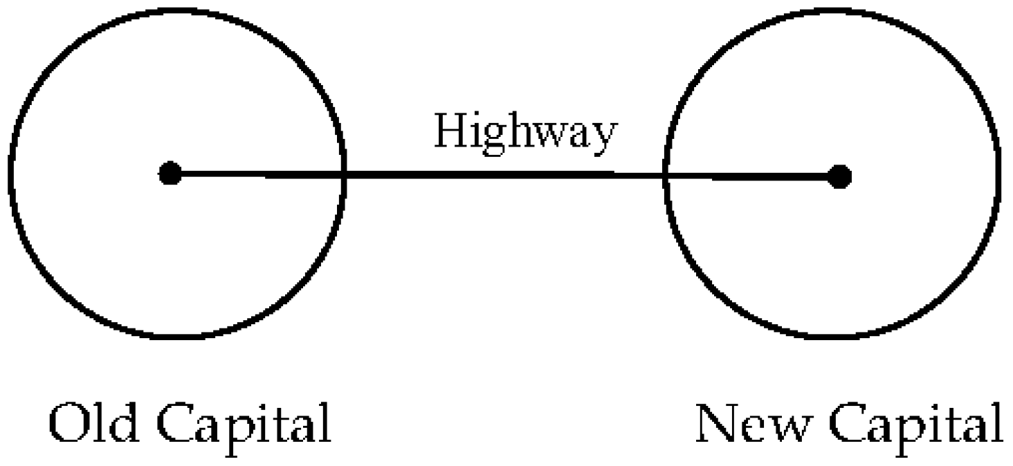
We assume a simple two-region (the old capital and the new capital, Figure 1) growth model based on Alonso (1964), Krugman (1991), and Sorek (2009). This model identifies the impacts of transportation and mobility costs on the regional economies [3,30,31]. Travel refers to mobility travel such as commuting and migration, with mobility costs. Commuting cost is incurred between two regions, but not within each region. Migration cost refers to the costs implicated in relocating. Commodities are traded between two regions, and so transportation cost, such as the shipping (trade) cost of commodities, is incurred in iceberg form. Each region produces different commodities. The labor input (worker) is assumed to be the only production factor. Agglomeration economies are represented as a function of the population. Commuting and migration costs, transportation cost, and total labor inputs are exogenous. Labor inputs can be disaggregated into four groups with respect to living and working locations. The four groups are as follows: living and working in the old capital; living and working in the new capital; living in the old capital, but working in the new capital; and the opposite of the third group.

Labor is supplied by the household. House members produce K + 1 times labor input in each house. The total population in each region is shown as in Equation (1). The size of the total population is fixed.

Population (Each region has non-zero population)

$$N_i={\displaystyle \sum _{j=1}^2{L}_{ij}(K+1)}$$

(1)

N_i: Population in region i;

L_ij: Labor input living in region i and working in region j;

K ≥ 0.

$$\overline{N}={\displaystyle \sum _{i=1}^2{N}_i}$$

(2)

Production is determined by a Cobb–Douglas function for labor inputs and agglomeration economies. The latter implies that the personal interactions involved in the production and output sales contribute to the productivity of firms. The price decreases with the population because g(N_i) represents scale effect, which represents agglomeration economies as urbanization economies, as measured by population in each region [32]. In this study, the population size is affected by relocation decisions, depending on transportation cost and mobility costs. Each household supplies homogenous labor, and the total labor inputs refer to the total man/hour. In terms of living and working locations in

Table 1. Four groups with respect to living and working locations.

Case I	Case II	Case III	Case IV
(1, 1)	(1, 2)	(2, 1)	(2, 2)
living and working in the old capital	living in the old capital, but working in the new capital	living in the new capital, but working in the old capital	living and working in the new capital

Note: (i, j) = (living, working).

, for example, output X in the old capital is produced by L₁₁ (workers living and working in the old capital) and L₂₁ (workers living in the new capital, but working in the old capital).

Production

$$X_i=Ag(N_i){L_{ii}}^{\delta }{L_{ji}}^{\theta }(j\ne i)$$

(3)

X_i: Aggregate output in region i;

A_i: Scale factor;

L_ii: Labor input living and working in region i;

L_ji: Labor input living in region j and working in region i;

g(N_i): Agglomeration economies function of population in region i;

δ + θ = 1;

0 < δ, θ < 1.

Firms maximize their profit. The conditional input demand functions for each worker are as follows under perfect competition.

Demand of each worker in region i

$$L_{ii}=\frac{\delta X_i{p}_i}{w_i}$$

(4)

$$L_{ji}=\frac{\theta X_i{p}_i}{w_i}(j\ne i)$$

(5)

Price in region i

$$p_i=\frac{w_i}{Ag(N_i){\delta }^{\delta }{\theta }^{\theta }}$$

(6)

Only the household is assumed to supply labor and consume the commodities in each house in this model. Consumers maximize the utility to consume two different regional commodities. The regional import is consumed at the transportation cost-inclusive price because of the shipping (trade) of the commodities. The transportation cost (t) is assumed to be greater than 0.

Utility

$$U_{ij}={z_{ij}^i}^{{\alpha }_{ij}}{z_{ij}^k}^{{\beta }_{ij}}(i\ne k)$$

(7)

zⁱ_ij: Commodities produced in region i that are consumed by workers living in region i and working in region j;

z^k_ij: Commodities produced in region k that are consumed by workers living in region i and working in region j;

α_ij + β_ij = 1;

0 < α_ij, β_ij < 1.

The household income is determined by the wage level. Total monthly income of a household is shown in Equation (8).

$$y_{ij}=w_{j}H-2d{c}_{ij}-m_{ij}$$

(8)

where y_ij is the monthly income of the household, excluding the mobility costs. H indicates the total monthly working time. This study did not adopt a time constraint, because a simple two-region growth model was used instead of a time-extended model. In addition, d is the working days in a month, and c_ij represents the commuting cost between the two regions. m_ij is the migration cost, which is incurred only when the living site is changed. Consequently, the budget constraint function of the household is shown in Equation (9). In addition, the Marshallian demands for each commodity are presented in Equations (11) and (12).

Demand of the house

$$y_{ij}=p_i{z}_{ij}^i+p_i^{\prime }{z}_{ij}^k$$

(9)

$$p_i^{\prime }=p_k{t}_{ki}$$

(10)

$$z_{ij}^i=\frac{{\alpha }_{ij}{y}_{ij}}{p_i}$$

(11)

$$z_{ij}^k=\frac{{\beta }_{ij}{y}_{ij}}{p_i^{\prime }}$$

(12)

where p_i is the price of a commodity in region i, and p’_i represents the price of a commodity in region k (p_k) plus the transportation cost from region k to region i (t_ki). Finally, the maximized utility level (U_ij = V_ij + ε_ij) is derived from Equation (13).

$$V_{ij}=\frac{{\alpha }_{ij}^{{\alpha }_{ij}}{\beta }_{ij}^{{\beta }_{ij}}{y}_{ij}}{p_i^{{\alpha }_{ij}}{(p_i^{\prime })}^{{\beta }_{ij}}}$$

(13)

The choice of living and working locations could be achieved through the maximized utility, Equation (13). This choice could be specified in the form of a probability. Assuming that ε_ij is independently identically distributed and follows Gumbel distribution (mean, zero, and variance, σ²: σ² = π²/6λ²), the choice probability of living and working sites is equal to Equation (14). λ is called the taste heterogeneity parameter. If λ approaches infinity (∞), the taste heterogeneity disappears.

$${\psi }_{ij}=\frac{\exp \lambda V_{ij}^{*}}{{\displaystyle \sum _{\forall (k,s)}\exp \lambda V_{ks}^{*}}}(j\ne i)$$

(14)

The probability that a randomly identified household chooses the living and working sites (i, j) to maximize the utility is calculated with the quadrinomial logit model (Pr_ij = Prob [U_ij > U_ks; ∀(i, j) ≠ (k, s)] = Prob [V_ij + ε_ij > V_ks + ε_ks; ∀(i, j) ≠ (k, s)], ∑ Pr_ij = 1) [14].

The expected welfare measure can be expressed as follows:

$$W=E[\underset{\forall (i,j)}{\max }{U}_{ij}]=\frac{1}{\lambda }\ln {\displaystyle \sum _{i,j}\exp (\lambda V_{ij})}$$

(15)

The general equilibrium is computed from the market clearing for output, labor, and competitive market.

Product market

$$X_k={\displaystyle \sum _{i,j,k}L{\psi }_{ij}}{z}_{ij}^k$$

(16)

Labor market

$$L_{ii}+L_{ji}={\displaystyle \sum _{k,i}L{\psi }_{ki}H}$$

(17)

Competitive market

$$p_i-\frac{w_i}{Ag(N_i){\delta }^{\delta }{\theta }^{\theta }}=0$$

(18)

4. Comparative Analysis

4.1. Transportation and Mobility Costs and Utilities

We assume two alternative mobility scenarios with regard to workers and population mobility from the original case of living and working in the old capital. The symmetric spatial distribution of population is initially assumed: N₁ = N₂.

Alternative I: Changing the working site from the old capital (i = 1) to the new capital (j = 2)

From L₁₁ to L₁₂, only the workers can change the working site through commuting. The population of the old capital does not change. The real income earned by a worker living in the old capital but working in the new capital decreases because of commuting cost c₁₂. The utility V₁₂ is negative in L₁₂. This result may be related to the commuting cost.

$$\frac{V_{11}}{V_{12}}=\frac{{\varphi }_{11}(A{e}^{-{\nu }_1/N_1}{\delta }^{\delta }{\theta }^{\theta }{p}_{1}H)}{{\varphi }_{12}(A{e}^{-{\nu }_2/N_2}{\delta }^{\delta }{\theta }^{\theta }{p}_{2}H-2d{c}_{12})}{p_1}^{-{\alpha }_{11}+{\alpha }_{12}}{(p_1^{\prime })}^{-{\beta }_{11}+{\beta }_{12}}$$

(19)

$$\frac{\partial V_{11}}{\partial L_{12}}>0,\frac{\partial V_{12}}{\partial L_{12}}<0,\frac{\partial V_{21}}{\partial L_{12}}>0,\frac{\partial V_{22}}{\partial L_{12}}<0$$

(${\varphi }_{ij}={\propto }_{ij}^{{\propto }_{ij}}·{\beta }_{ij}^{{\beta }_{ij}}$)

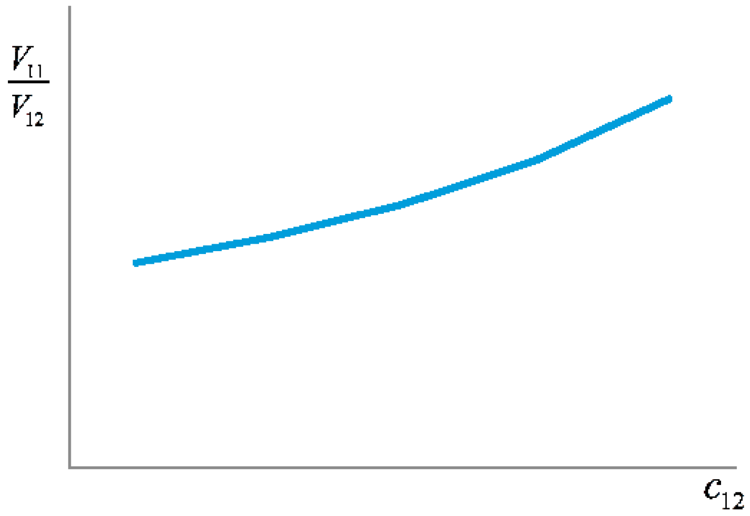
In this case, even if the workers’ mobility occurs, the total population in each region does not change. Additional subsidy or incentives are needed to induce commuting to the new capital on the condition of the utility V₁₁ < V₁₂ because 2dc₁₂ > w₂H. Figure 2 shows that the gap between two utilities increases according to the rising commuting cost. Commuting cost negatively affects the utility of workers living in the old capital, but working in the new capital.

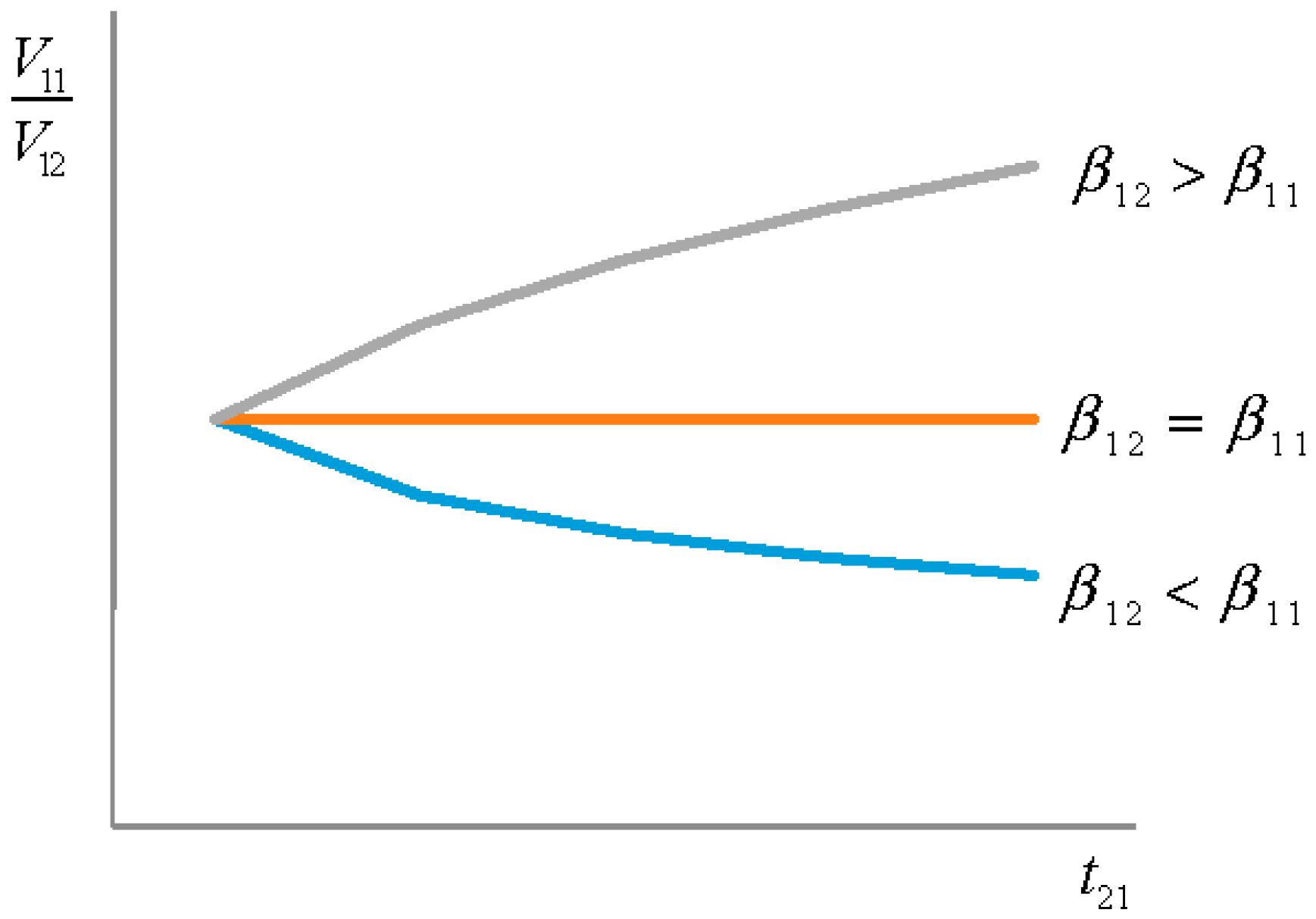
Figure 3 shows how the transportation cost affects the ratio of utilities. Transportation cost affects the real income and the commodity’s price. β₁₁ and β₁₂, the parameters of the preference for the commodity produced in the new capital, affect the ratio of the two utilities. If a worker who lives in the old capital but works in the new capital prefers the commodity produced in the new capital more than a worker who lives and works in the old capital, the gap of utilities increases with the transportation cost. The increasing transportation cost influences the price and affects the utility negatively. Additionally, the production of this commodity in the new capital increases, and ultimately raises the nominal wage in the new capital. This effect increases the welfare of the population, including the workers living in the old capital, but working in the new capital.

Alternative II: Migrating to the new capital and changing the working site

From L₁₁ to L₂₂, the population, including the workers, migrates to the new capital, and the working site also changes. The population in the new capital increases. The nominal wage in the new capital also increases, whereas the nominal wage in the old capital decreases. Migration cost is incurred. The utility V₂₂ is positive in L₂₂. This result is caused by the increasing wage in the new capital.

$$\frac{V_{11}}{V_{22}}=\frac{{\varphi }_{11}(A{e}^{-{\nu }_1/N_1}{\delta }^{\delta }{\theta }^{\theta }{p}_{1}H)}{{\varphi }_{22}(A{e}^{-{\nu }_2/N_2}{\delta }^{\delta }{\theta }^{\theta }{p}_{2}H-m_{22})}{p_1}^{-{\alpha }_{11}}{(p_1^{\prime })}^{-{\beta }_{11}}{(p_2^{\prime })}^{{\beta }_{22}}{p_2}^{{\alpha }_{22}}$$

(20)

$$\frac{\partial V_{11}}{\partial L_{22}}<0,\frac{\partial V_{22}}{\partial L_{22}}>0,\frac{\partial V_{12}}{\partial L_{22}}>0,\frac{\partial V_{21}}{\partial L_{22}}<0$$

Migration decreases the population in the old capital. It is possible that V₂₂ > V₁₁ if w₂H is larger than m₂ [N₂²/(N₁² + N₂²)]. If the household income is large enough to compensate for the migration cost without any subsidy or incentive, migration benefits the population, including the workers. Figure 4 shows that the gap between the two utilities increases according to the rising migration cost. Migration cost affects the utility of worker migrating to the new capital.

In Figure 5, as the transportation cost t₁₂ increases, the price of the commodity produced in the old capital increases. Hence, the utility of the workers living in the new capital after migration is negatively affected. The gap of utilities widens according to the increasing transportation cost t₁₂. However, when the transportation cost t₂₁ increases, the gap of utilities decreases. This result is related to the price of the commodity produced in the new capital, which the workers living and working in the old capital pay. This result negatively affects the utility V₁₁.

In summary, as the population including the workers migrates to the new capital, the nominal wage in the new capital increases, whereas the nominal wage in the old capital decreases. Utility is also directly related to the nominal wage or real income. Transportation cost negatively affects the price of the commodity and the utility. The effects of commuting and migration costs on the utility are negative. A financial subsidy is needed to enable workers to commute from the old capital to the new capital.

4.2. Agglomeration Effect and Utilities

Agglomeration economies arise from the total population in each region. The utility may be affected by agglomeration factors, parameters, and population size. The agglomeration effects of the increasing region size can induce urban costs, such as congestion or disamenity.

$$g(N_1)=e^{-{\nu }_1/N_1},g(N_2)=e^{-{\nu }_2/N_2}\mathrm{s}.\mathrm{t}.\nu >0$$

(21)

Alternative I: Changing the working site from the old capital (i = 1) to the new capital (j = 2)

$$V_{12}={\varphi }_{12}(A{e}^{-{\nu }_2/N_2}{\delta }^{\delta }{\theta }^{\theta }{p}_{2}H-2d{c}_{12}){p_1}^{-{\alpha }_{12}}{(p_1^{\prime })}^{-{\beta }_{12}}$$

(22)

In Alternative I, the population in each region is constant, and the utility changes in a declining degree or according to elasticity ν. The utility is opposite in ν. Thus, the utility of the workers living in the old capital but working in the new capital is affected only by a declining degree of agglomeration economies.

Alternative II: Migrating to the new capital and changing the working site

$$V_{22}={\varphi }_{22}(A{e}^{-{\nu }_2/N_2}{\delta }^{\delta }{\theta }^{\theta }{p}_{2}H-m_{22}){p_2}^{-{\alpha }_{22}}{(p_2^{\prime })}^{-{\beta }_{22}}$$

(23)

The population, including the workers, migrates to the new capital, and the working site also changes. Therefore, the population in the new capital increases. The utility of the workers living and working in the new capital increases due to the improved agglomeration effects. In the change of ν, the slope of the utility is less steep.

Finally, even if transportation and mobility costs negatively affect the utility, agglomeration economies improve in the increasing population through migration. The utility of the workers living and working in the new capital increases due to the improved agglomeration effects.

5. Numerical Simulation

Empirically, it is set that the old capital is Seoul, and the new capital is Sejong City (Sejong). The number of workers living in Seoul and Sejong are 11 million and 3.5 million, respectively. The initial data are obtained from Statistics Korea. This analysis discusses the spatial dispersion of workers depending on relocation decisions between Seoul and Sejong, as well as their effect on regional economies. The change in commuting and transportation cost is considered under static conditions. The dispersion of workers in each living and working site is interpreted as the change rate of the initial value set to 100. 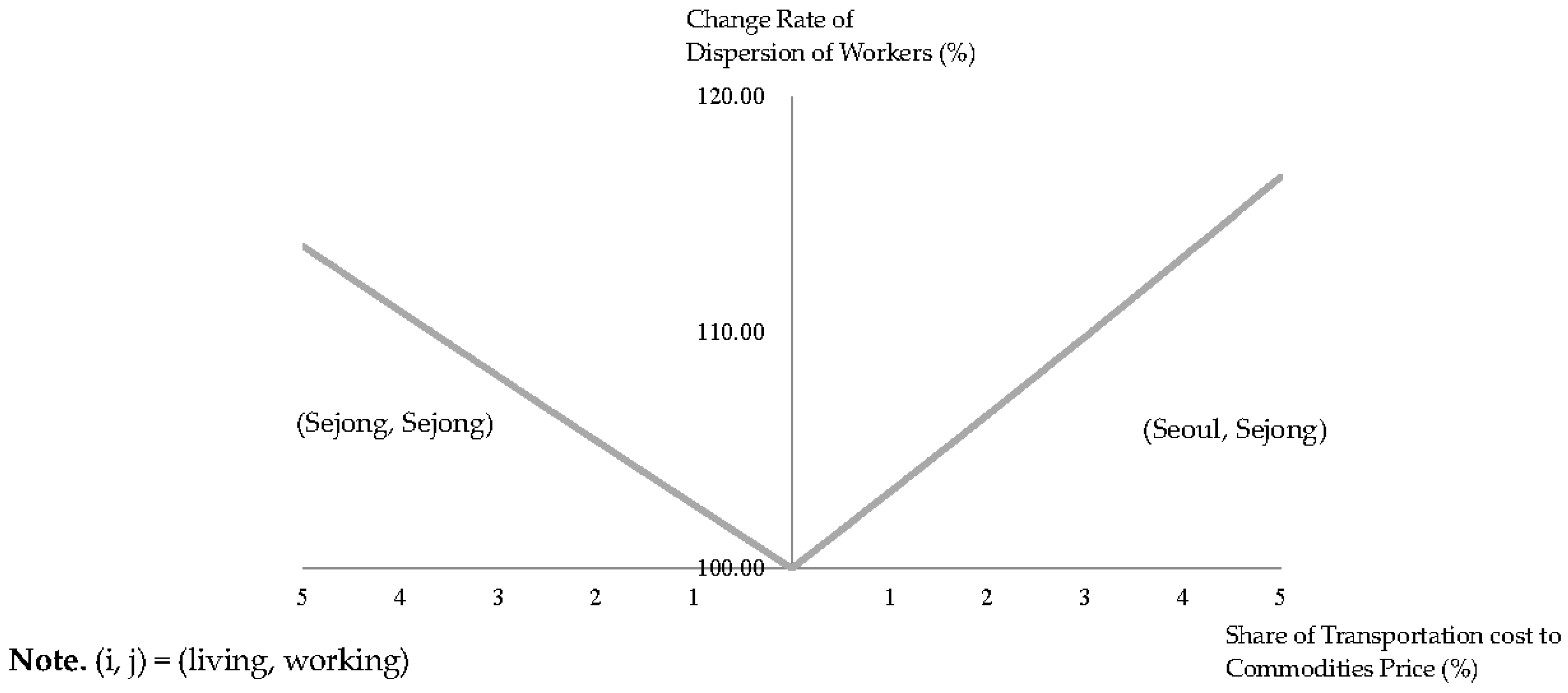Figure 6 and Figure 7 illustrate the effects of change in commuting and transportation cost on the dispersion of workers, respectively. The first dimension indicates the case of living in Seoul, but working in Sejong. The second dimension is the case of living and working in Sejong. The change rate of the dispersion of workers steeply responds to the change in transportation cost, as shown in Figure 7. As the commuting cost increases, the number of workers living and working in Sejong sharply increases. However, the choice probability of living in Seoul, but working in Sejong increases marginally, despite the commuting cost.

In conjunction with Figure 6, Figure 8 shows the relationship between the change of workers living in Seoul but working in Sejong, and the change of commuting cost. This indicates that commuting stops when the monthly commuting cost exceeds 1290 USD—about 26.1% of the monthly average income of urban households with four members in Korea—at constant price. The higher commuting cost results in the dispersion of workers to Sejong. This implies that the population may increase naturally and foster the economic activities in Sejong.

Figure 9 shows the positive relationship between the number of workers living in Sejong and the higher transportation cost. This implies the dispersion of workers from Seoul to Sejong. Krugman (1991) and Kilkenny (1998) proved that the concentration in the old capital is favored by the reduction in transportation cost [6,31], while Murata and Thisse (2005) suggested that a higher transportation cost fosters labor concentration and agglomeration in the region [9]. At a lower transportation cost, more workers live in Seoul, and the population ultimately increases. Originally, 11 million workers, out of the total 14.5 million workers in the two regions, live in Seoul. However, since transportation cost is rising, the number of workers living in Sejong is increasing. If the share of transportation cost to commodity’s price reaches up to 60.1%, the workers will be balanced between Seoul and Sejong.

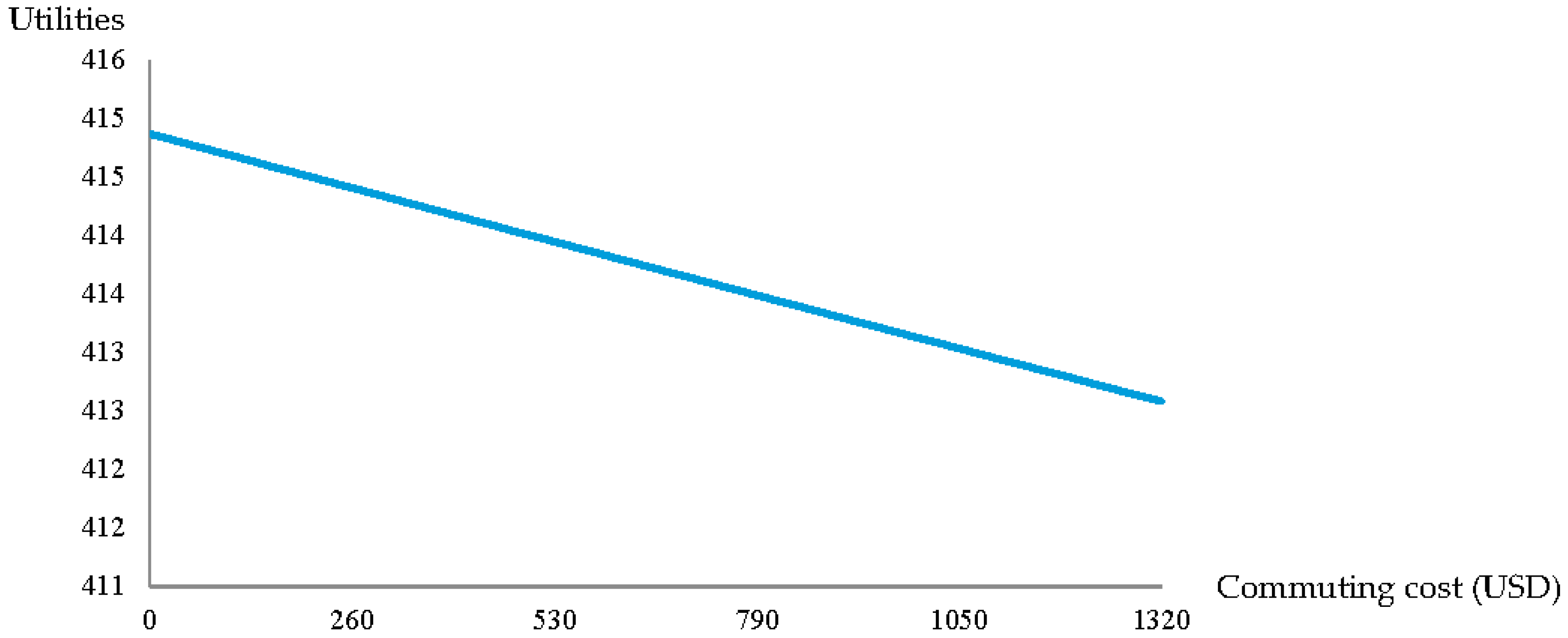
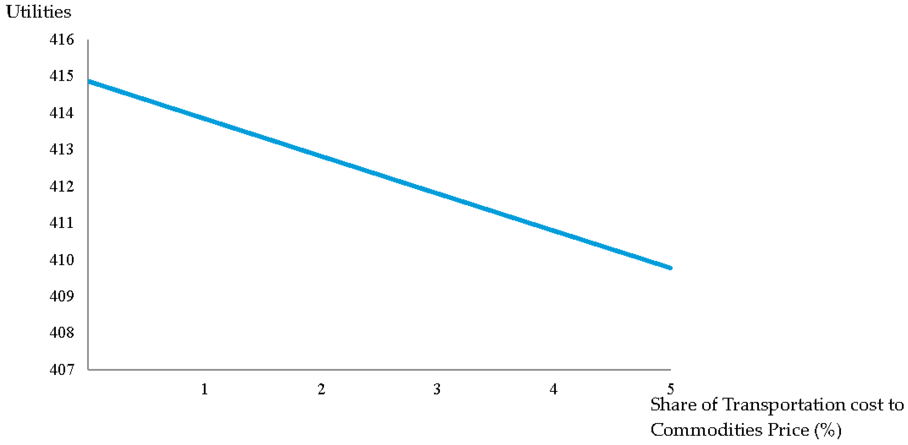
Figure 10 and Figure 11 illustrate the relationship between the transportation or commuting cost and utilities. The higher transportation or commuting cost negatively affects the utilities, even if they contribute to the dispersion of workers. The effect of increasing transportation cost on utilities is greater than that of increasing commuting cost.

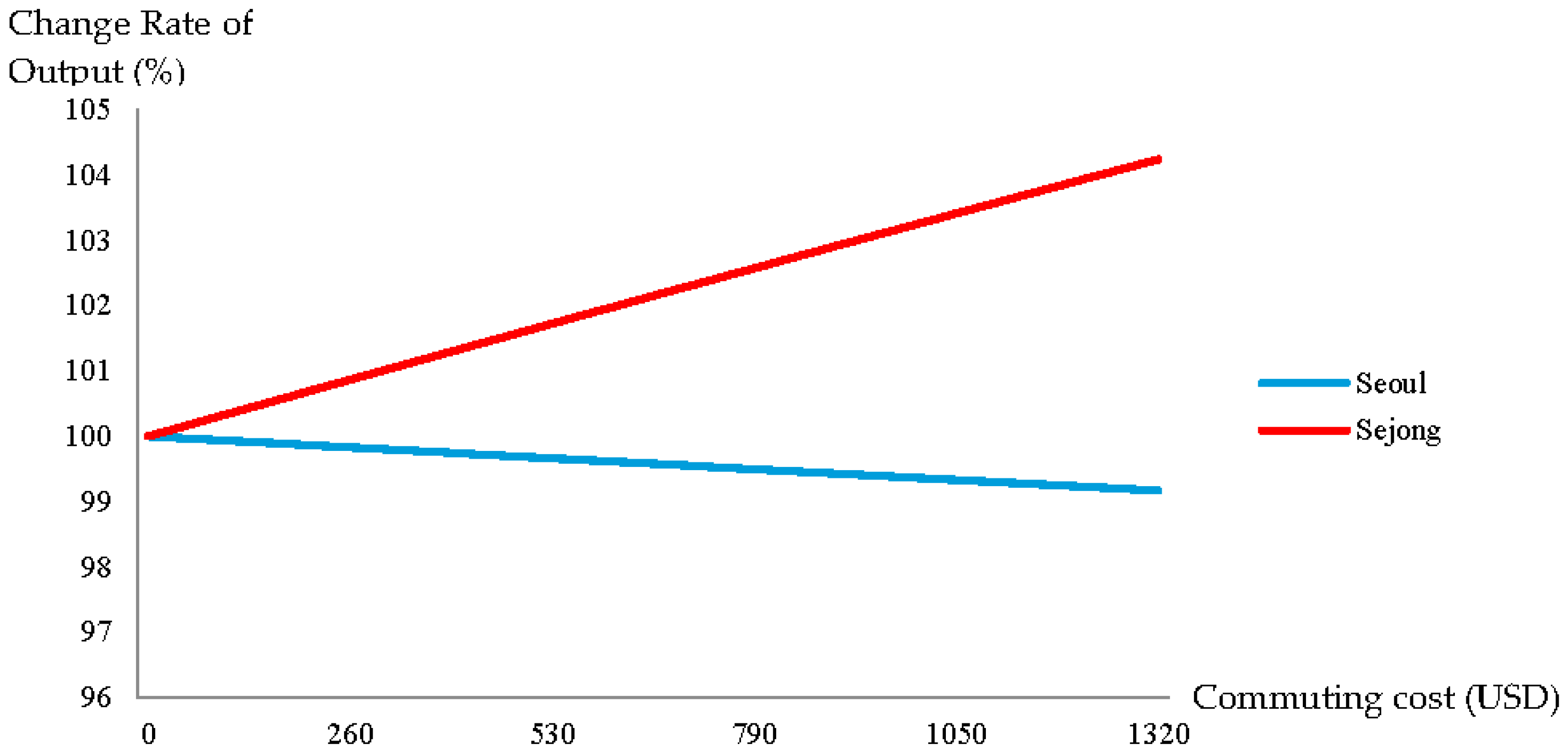
Figure 12 and Figure 13 show that output in Sejong increases with the rising transportation and commuting cost. This is related to the scale effect of agglomeration economies.

Consequently, the lower transportation and commuting costs foster the concentration of workers in Seoul. Paradoxically, the higher transportation and commuting costs induce the dispersion of workers to Sejong, and positively affect the output growth. However, the social welfare decreases, as indicated by Kilkenny (1998) [6]. Kilkenny (1998) pointed out that rural development could only be achieved at a lower overall welfare [6]. In the sense that 1290 USD is the maximum amount for the commuters to pay from Seoul to Sejong, the government needs to restrict the financial subsidy allocated to them in order to increase the population size of Sejong. If the share of transportation cost to commodity price reaches 60.1%, the interregional population equilibrium could be achieved. In addition, for the sustainable growth of Sejong, it is necessary to implement in-migration policy tools such as improvement of living quality (e.g., housing supply and amenities) and the development of public infrastructure facilities (e.g., transportation and disaster prevention).

6. Conclusions

This paper analyzes the effects of transportation and mobility costs on the mobility of workers and population between the old and new capital cities using a two-region growth model. First of all, there is clearly a negative effect of transportation and mobility costs on utility, and the agglomeration economies in Sejong (the new capital) could improve with increasing population through migration. These agglomeration economies positively lead to output growth with scale effect. Higher transportation and commuting costs could result in the spatial dispersion of workers. In addition, if the monthly commuting cost exceeds 1290 USD between the old and new capital cities, it would be efficient for workers in Seoul to move to Sejong. Finally, the interregional population equilibrium could be achieved when the share of transportation cost to commodity price reaches 60.1%. This result can identify what kinds of financial subsidies and policy tools on population and commuters are necessary for the mutual development of a few core cities such as old and new capital cities in terms of population distribution. What is an effect of the commuter cost on the population dispersion between the cities? What are the effectiveness and efficiency of regional development tools with respect to spatial income disparity? How does spatial accessibility from the infrastructure development affect regional economic integration? In particular, the impact of transportation costs on the mobility from this paper could contribute to policy formulation and processes of population and location of Japan, Indonesia, and other countries that have discussed the construction of a new administrative capital city.

As for further research issues, one is to quantify the time value and mobility costs in monetary terms. It would be interesting to extend the two-region growth model to a dynamic one with forward-looking behavior of households, producers, and national and local governments between overlapping generations. Another future research area could be exploring the optimal size of the population through using agglomeration economies and scale effects of distances and factor inputs. Since actual relocation patterns take the form of polycentric cities, it is necessary to specify a spatial model with multiple workplaces and residential areas in mixed urban structures, the heterogeneous quality of schooling, and urban functions for QOL [33].

References

1. Lim, J.W.; Lee, C.K.; Kim, E.J. Contributions of human capital investment policy to regional economic growth: An interregional CGE model approach. Ann. Reg. Sci. 2015, 55, 269–287. [Google Scholar] [CrossRef]
2. Pinto, S.M. Residential Choice, Mobility, and the Labor Market. J. Urban Econ. 2002, 51, 469–496. [Google Scholar] [CrossRef]
3. Sorek, G. Migration costs, commuting costs and intercity population sorting. Reg. Sci. Urban Econ. 2009, 39, 377–385. [Google Scholar] [CrossRef]
4. Wrede, M. Should Commuting Expenses Be Tax Deductible? A Welfare Analysis. J. Urban Econ. 2001, 49, 80–99. [Google Scholar] [CrossRef]
5. Fujita, M.; Krugman, P.; Venables, A.J. The Spatial Economy; MIT Press: Cambridge, MA, USA, 1999. [Google Scholar]
6. Kilkenny, M. Transport costs and Rural Development. J. Reg. Sci. 1998, 38, 293–312. [Google Scholar] [CrossRef]
7. Tabuchi, T.; Thisse, J.F.; Zeng, D.Z. On the number and size of cities. J. Econ. Geogr. 2005, 5, 423–448. [Google Scholar] [CrossRef]
8. Tabuchi, T. Urban Agglomeration and dispersion: A Synthesis of Alonso and Krugman. J. Urban Econ. 1998, 44, 333–351. [Google Scholar] [CrossRef]
9. Murata, Y.; Thisse, J.F. A simple model of economic geography à la Helpman-Tabuchi. J. Urban Econ. 2005, 58, 137–155. [Google Scholar] [CrossRef]
10. Alstadt, B.; Weisbrod, G.; Cutler, D. The Relationship of Transportation Access and Connectivity to Local Economic Outcomes: A Statistical Analysis. In Proceedings of the Transportation Research Board Annual Conference, Washington, DC, USA, 22–26 January 2012. [Google Scholar]
11. Allio, C. Inter urban population distribution and commute modes. Ann. Reg. Sci. 2016, 57, 125–144. [Google Scholar] [CrossRef]
12. Suh, S.H. The Possibility and impossibility of intercity commuting. J. Urban Econ. 1988, 23, 86–100. [Google Scholar] [CrossRef]
13. Anas, A.; Arnott, R.; Small, K.A. Urban spatial structure. J. Econ. Lit. 1998, 36, 1426–1464. [Google Scholar]
14. Anas, A.; Rhee, H.J. When are urban growth boundaries not second-best policies to congestion tolls? J. Urban Econ. 2007, 61, 263–286. [Google Scholar] [CrossRef]
15. Baum-Snow, N. Did highways cause suburbanization? Q. J. Econ. 2007, 122, 775–805. [Google Scholar] [CrossRef]
16. Baum-Snow, N. Suburbanization and transportation in the monocentric model. J. Urban Econ. 2007, 62, 405–423. [Google Scholar] [CrossRef]
17. Xu, H.; Li, Z. High-Speed Railroad and Economic Geography: Evidence from Japan; Asian Development Bank Economics Working Papers; Asian Development Bank: Metro Manila, Philippines, 2016; No. 485. [Google Scholar]
18. Harris, J.R.; Todaro, M.P. Migration and Unemployment: A Two-Sector Analysis. Am. Econ. Rev. 1970, 60, 126–142. [Google Scholar]
19. Todaro, M.P. A Model of Labor Migration and Urban Unemployment in Less Developed Countries. Am. Econ. Rev. 1969, 59, 138–148. [Google Scholar]
20. Cristopher, A.P.; McMaster, I. Regional Migration, Wages and Unemployment: Empirical Evidence and Implication for Policy. Oxf. Econ. Pap. 1990, 42, 812–831. [Google Scholar]
21. Cushing, B.; Poot, J. Crossing Boundaries and Borders: Regional Science Advantages in Migration Modelling. Pap. Reg. Sci. 2004, 83, 317–338. [Google Scholar] [CrossRef]
22. Kancs, A. The economic geography of labor migration: Competition, competitiveness and development. Appl. Geogr. 2011, 31, 191–200. [Google Scholar] [CrossRef]
23. Tiebout, C. A pure theory of local public expenditures. J. Political Econ. 1956, 64, 416–424. [Google Scholar] [CrossRef]
24. Porell, F.W. Inter-metropolitan Migration and Quality of Life. J. Reg. Sci. 1982, 22, 137–158. [Google Scholar] [CrossRef] [PubMed]
25. Marshall, J.N.; Bradley, D.; Hodgson, C.; Alderman, N.; Richarson, R. Relocation, relocation, relocation: Assessing the case for public sector dispersal. Reg. Stud. 2005, 39, 767–787. [Google Scholar] [CrossRef]
26. McKinnish, T. Welfare-induced migration at state borders: New evidence from Micro-data. J. Public 2007, 91, 437–450. [Google Scholar] [CrossRef] [PubMed]
27. Glazer, A.; Kanniainen, V.; Poutvaara, P. Income taxes, property values, and migration. J. Public Econ. 2008, 92, 915–923. [Google Scholar] [CrossRef]
28. Koethenbuerger, M. Competition for migrants in a federation: Tax or Transfer competition? J. Urban Econ. 2014, 80, 110–118. [Google Scholar] [CrossRef]
29. Rijnks, R.H.; Koster, S.; McCann, P. Spatial Heterogeneity in Amenity and Labor Market Migration. Int. Reg. Sci. Rev. 2016, 1–27. [Google Scholar] [CrossRef]
30. Alonso, W. Location and Land Use; Easr-West Center: Honolulu, HI, USA, 1964. [Google Scholar]
31. Krugman, P. Increasing Returns and Economic Geography. J. Political Econ. 1991, 99, 483–499. [Google Scholar] [CrossRef]
32. Eberts, R.W.; McMillen, D.P. Agglomeration Economies and Urban Public Infrastructure. In Handbook of Regional and Urban Economics, 1st ed.; Cheshire, P., Mills, E.S., Eds.; Elsevier: Amsterdam, The Netherlands, 1999; Volume 3, pp. 1455–1495. [Google Scholar]
33. Hanushek, E.A.; Yilmaz, K. Schools and Location: Tiebout, Alonso, and Governmental Finance Policy. J. Public Econ. Theory 2013, 15, 829–855. [Google Scholar] [CrossRef]
Figure 1. Structure of the two-region model.
Sustainability 09 01872 g001
Figure 2. Commuting cost and utilities.
Sustainability 09 01872 g002
Figure 3. Transportation cost and utilities.
Sustainability 09 01872 g003
Figure 4. Migration cost and utilities.
Sustainability 09 01872 g004
Figure 5. Transportation cost and utilities.
Sustainability 09 01872 g005
Figure 6. Effect of change in communing cost on the dispersion of workers.
Sustainability 09 01872 g006
Figure 7. Effect of change in transportation cost on the dispersion of workers.
Sustainability 09 01872 g007
Figure 8. Change of workers living in Seoul but working in Sejong.
Sustainability 09 01872 g008
Figure 9. Transportation cost and dispersion of workers between the two regions.
Sustainability 09 01872 g009
Figure 10. Impact of change in commuting cost on utilities.
Sustainability 09 01872 g010
Figure 11. Impact of change in transportation cost on utilities.
Sustainability 09 01872 g011
Figure 12. Impact of change in commuting cost on output.
Sustainability 09 01872 g012
Figure 13. Impact of change in transportation cost on output.
Sustainability 09 01872 g013