Application of Kalman Filter for Estimating a Process Disturbance in a Building Space


Abstract
:1. Introduction
- In most buildings, occupancy information of each space is not collected because of the privacy issue. Moreover, the sensible and latent heat gain from people vary according to age, sex, and activities [1].
- Electric consumption by lights and equipment (PCs, laptops, printers, etc.) is not generally sub-metered. Moreover, heat release from those varies depending on their types, specifications, and part load [1].
- It is difficult to measure the airflows by infiltration, ventilation, and air movement between zones) in each space [2].
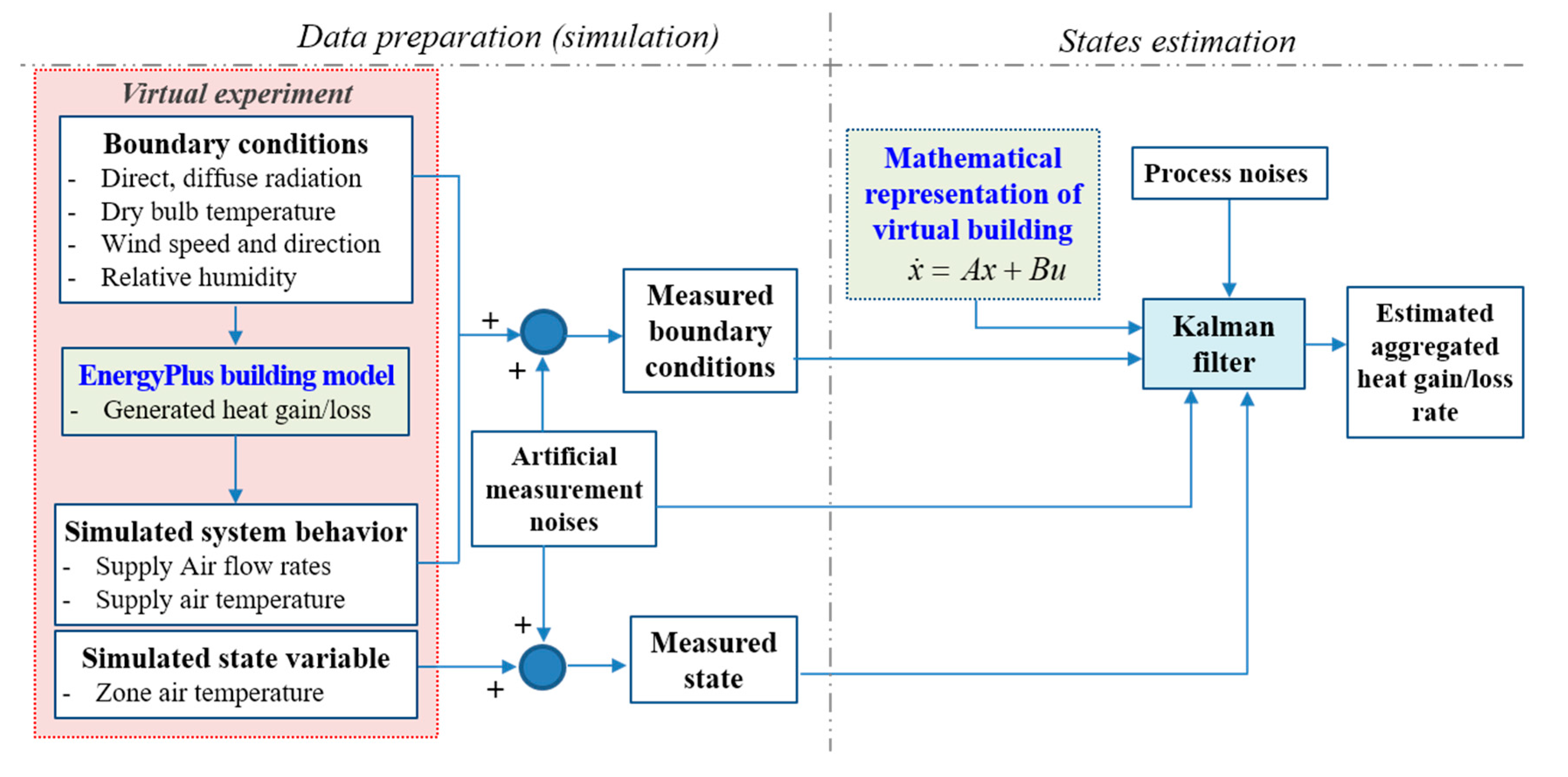
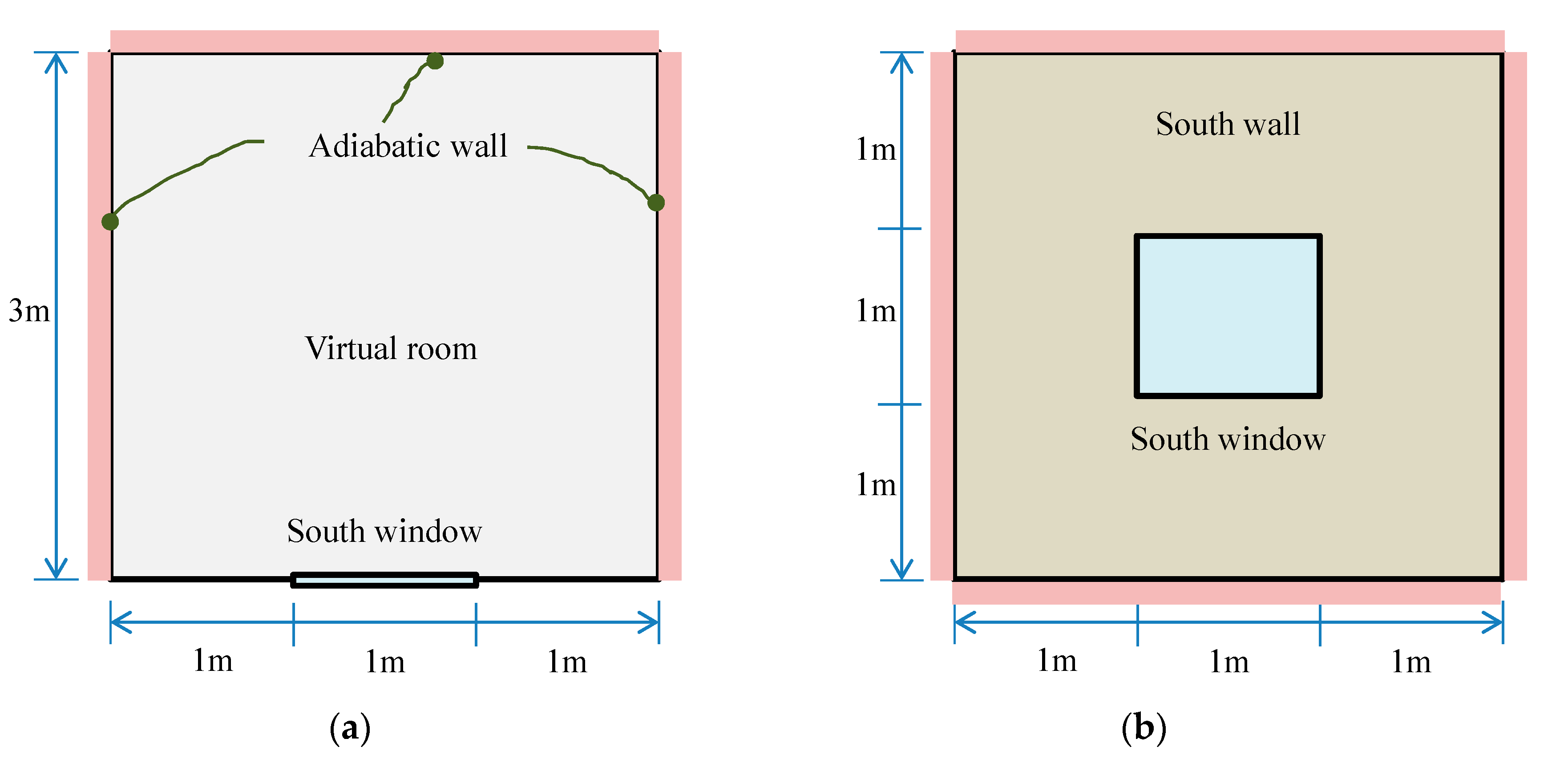
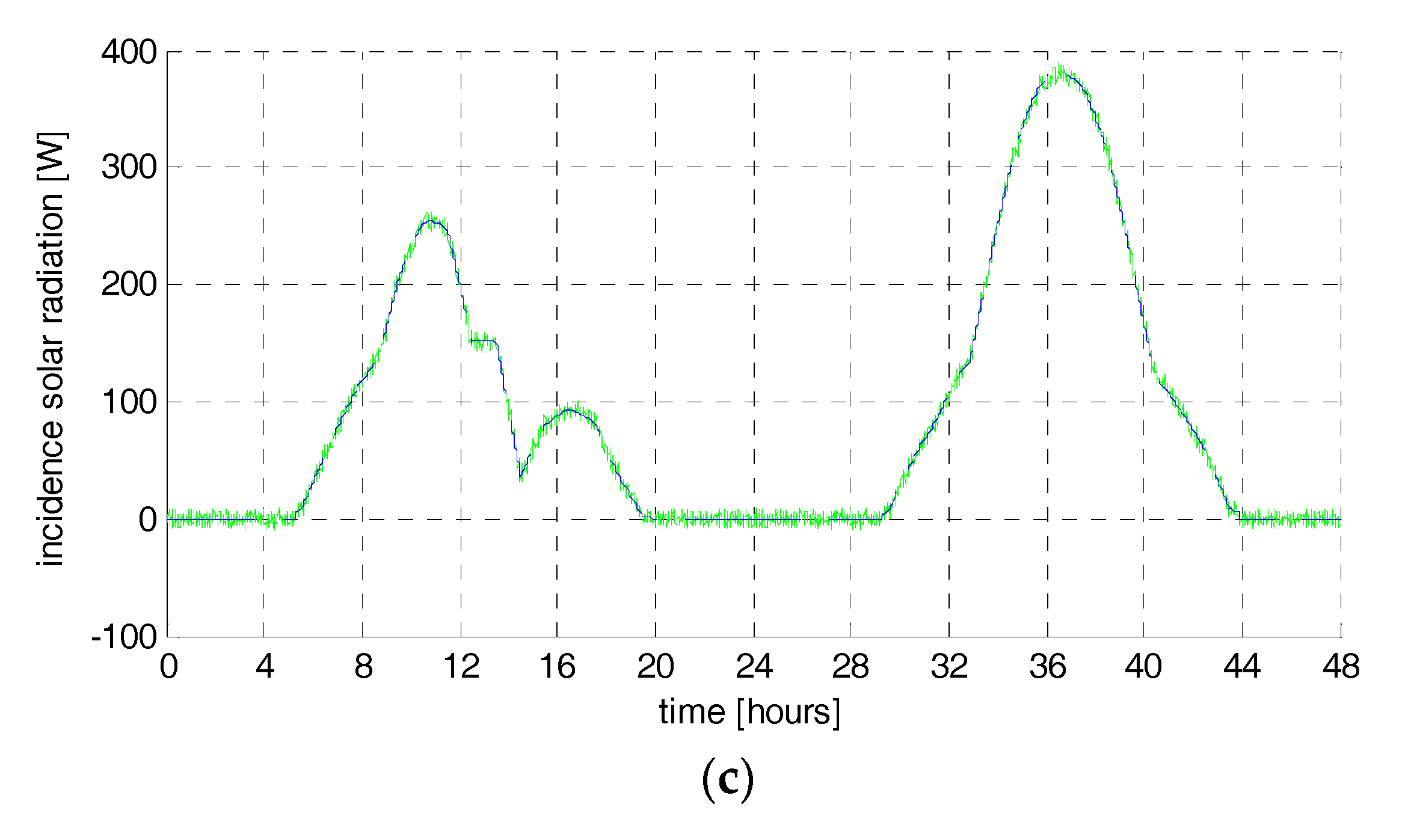
- Virtual experiment—a single room simulation model (3 m high, 3 m wide and 3 m deep) was made under a clear sky condition in two summer days. The time-varying aggregated heat gain/loss rate was manipulated inside the full dynamic simulation model. Four simulation cases were designed to test the KF estimation performance with regard to the heat gain/loss rate of the simulation room model.
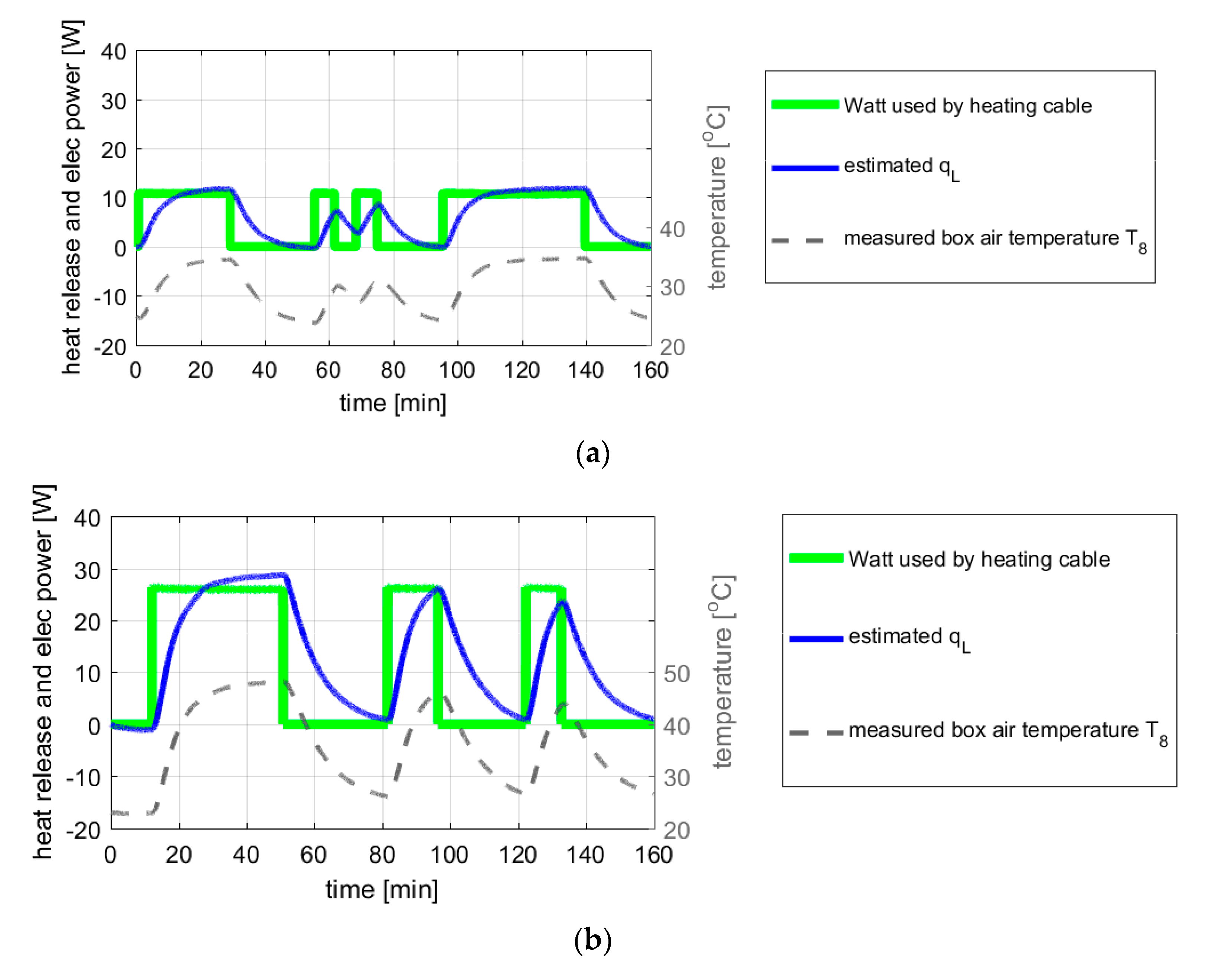
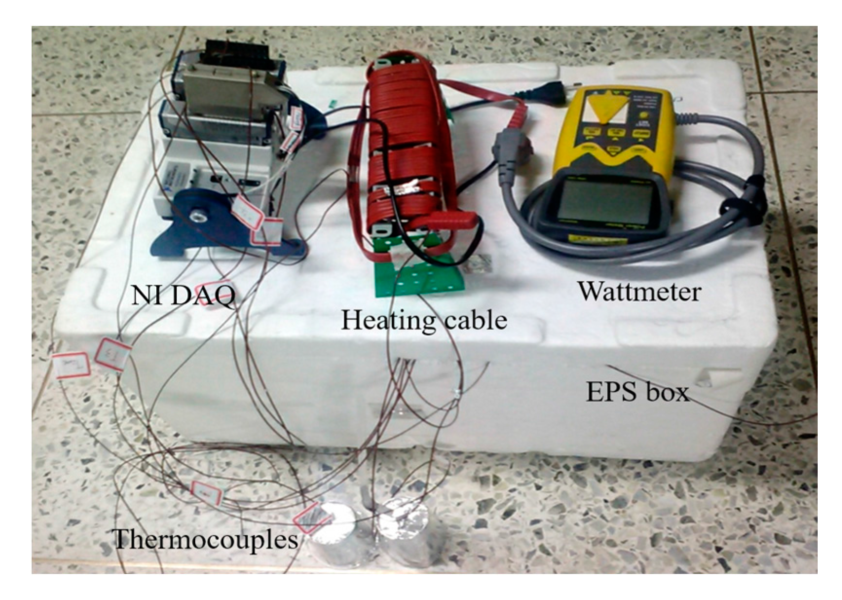
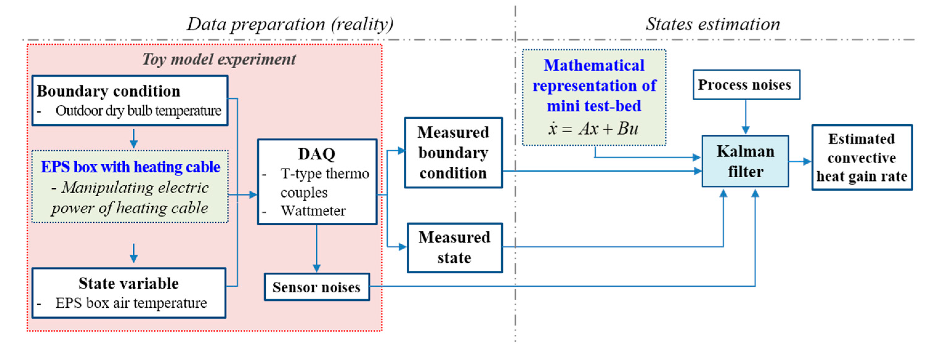
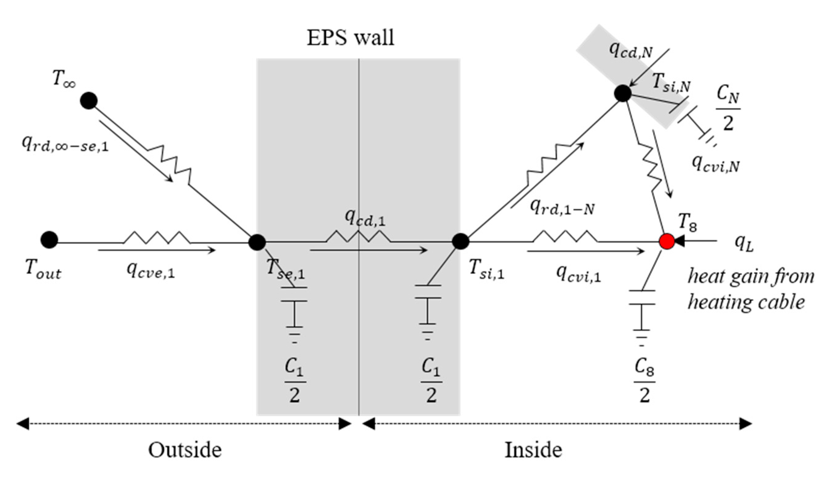
- Mini test-bed experiment—a small-scale real experiment was conducted in a rectangular box made of expanded polystyrene. The box represents a room space and electric heating cables installed inside the box emulates a convective heating system. Two experimental cases were conducted to test the KF estimation performance of time-varying electrical heat releases from the cables.
2. Kalman Filtering
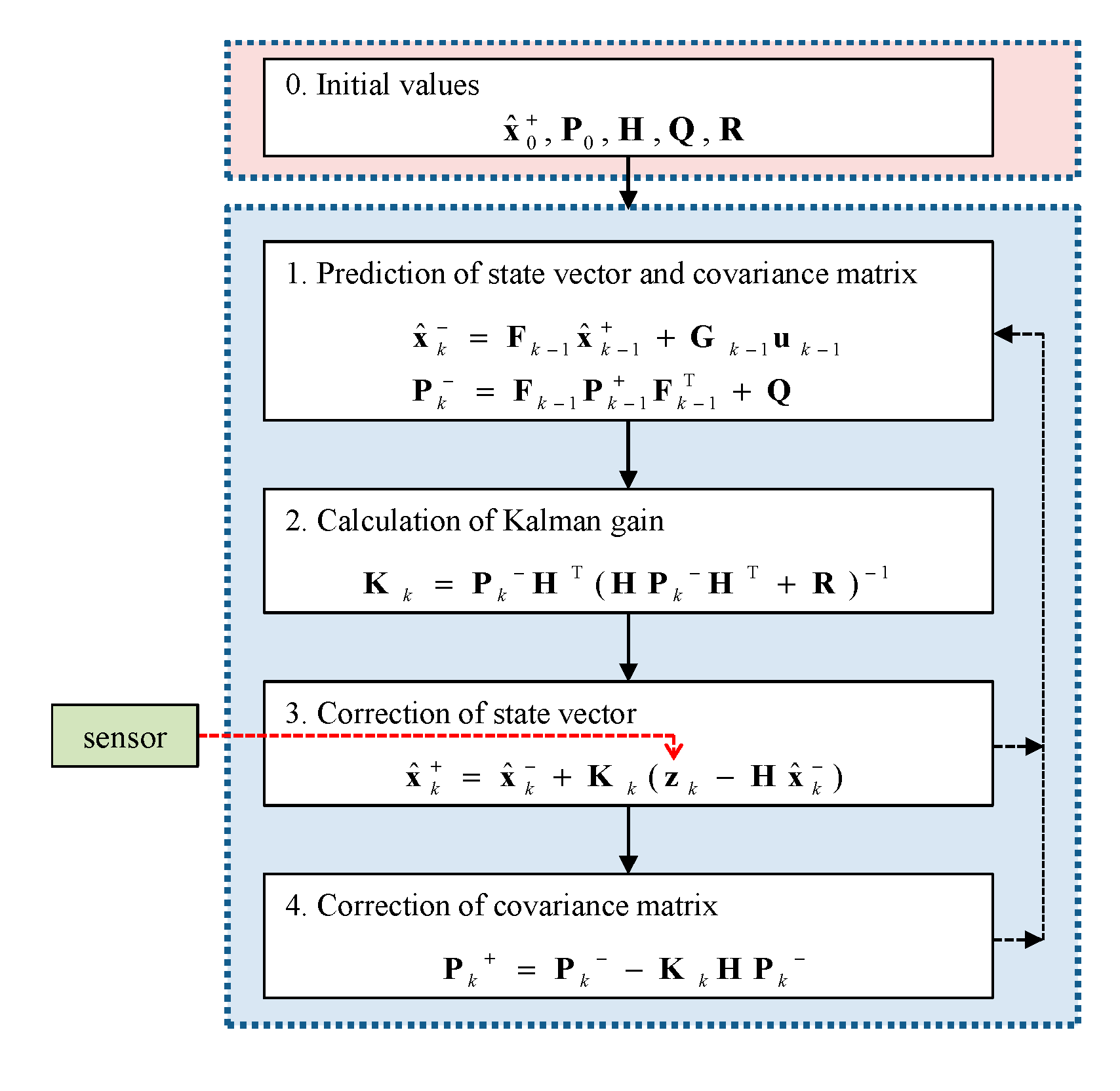
2.1. Algorithm
2.2. State Augmentation
2.3. Random Walk Hypothesis for the Process Disturbance
3. Virtual Experiment
3.1. Simulation Model by EnergyPlus
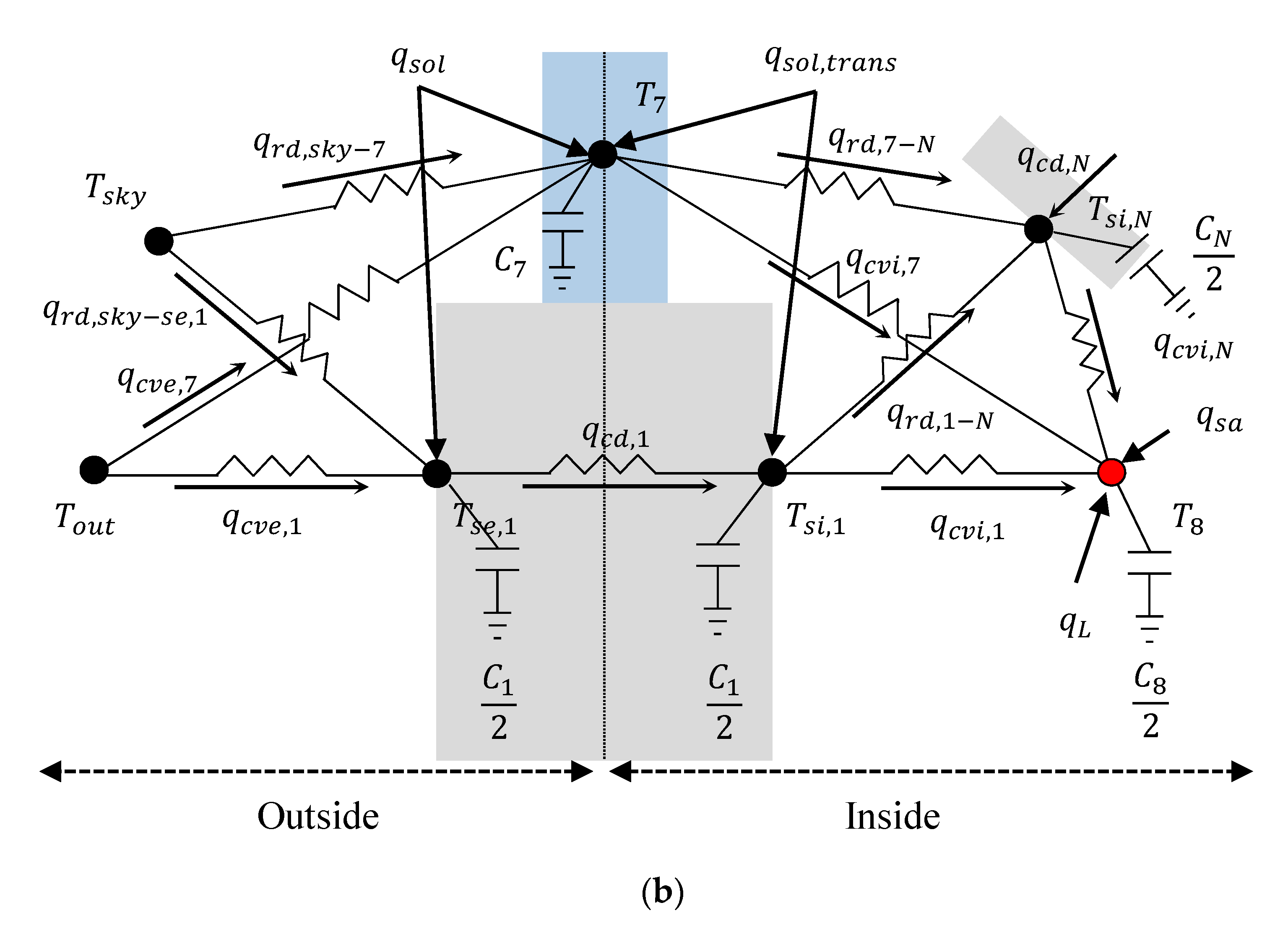
3.2. Augmented State-Space Model Resembling EnergyPlus Simulation Model
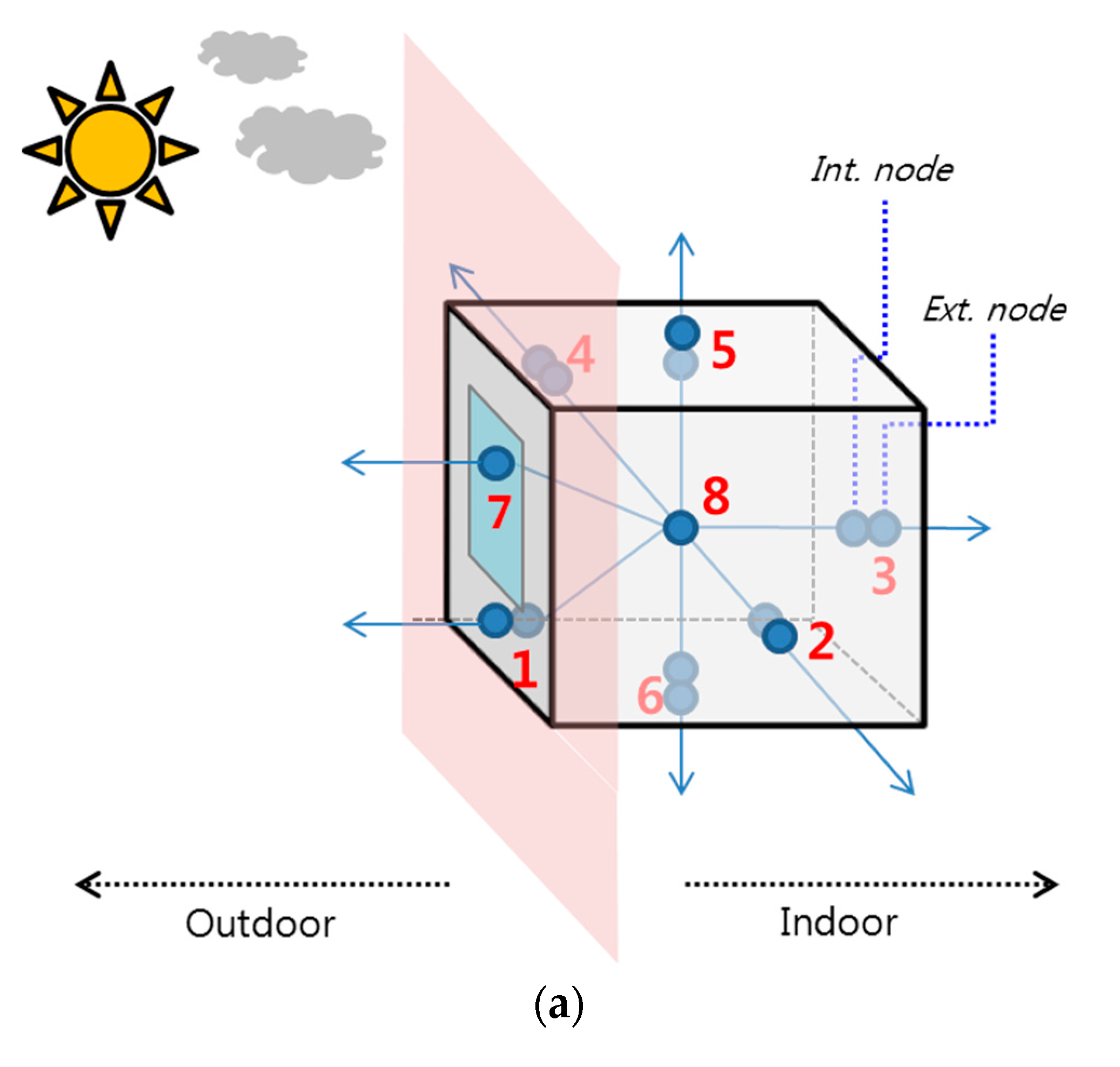
- The 1st to 8th states represent the interior and exterior surface nodes of the walls (the surface numbers from #1 to #4 in Figure 5a)
- The 9th to 12th states represent the interior and exterior surface nodes of the ceiling and the floor (the surface numbers from #5 to #6 in Figure 5a)
- The 13th state is the window node (the window is assumed to be one node)
- The 14th state is the zone air node
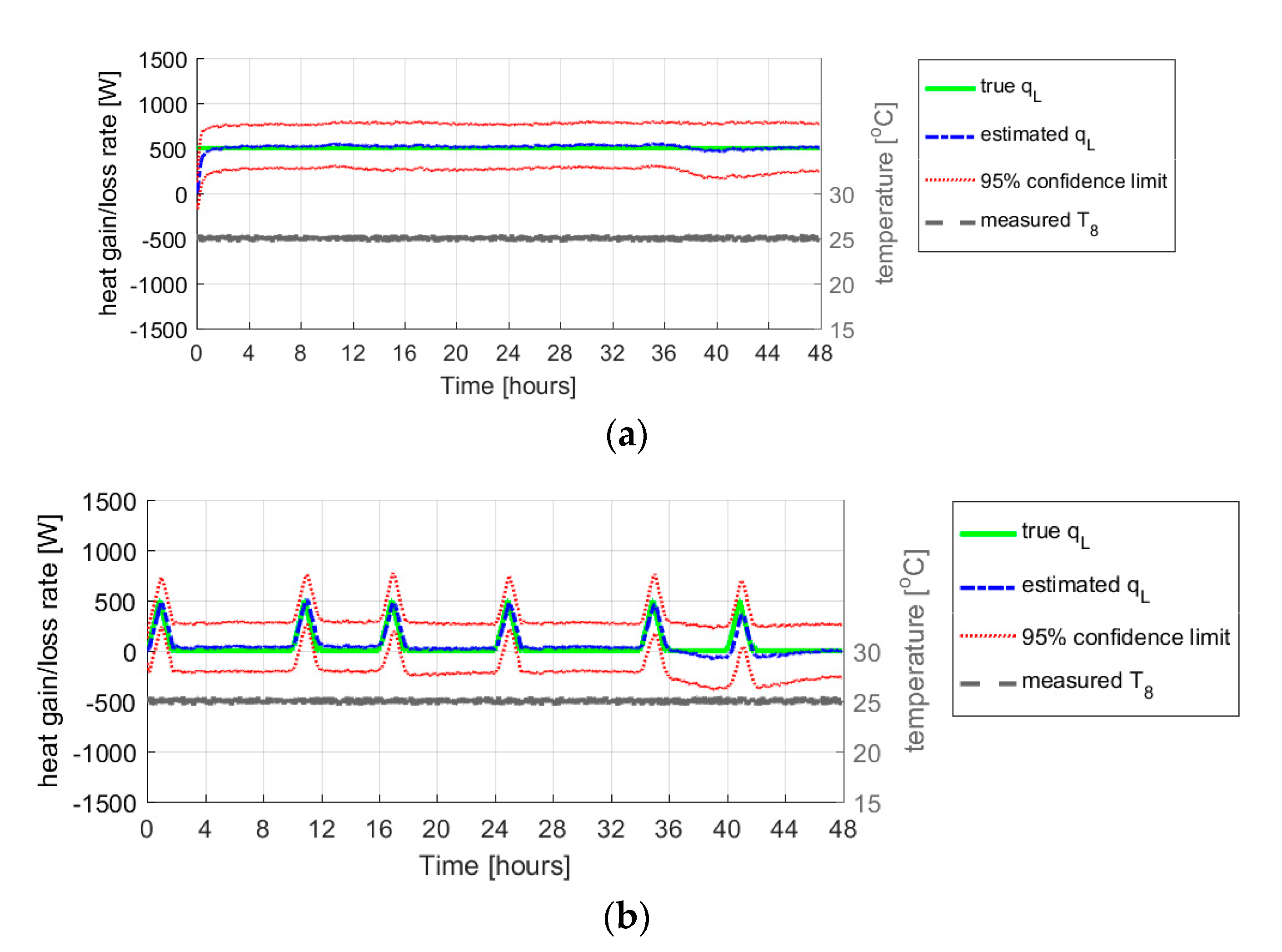
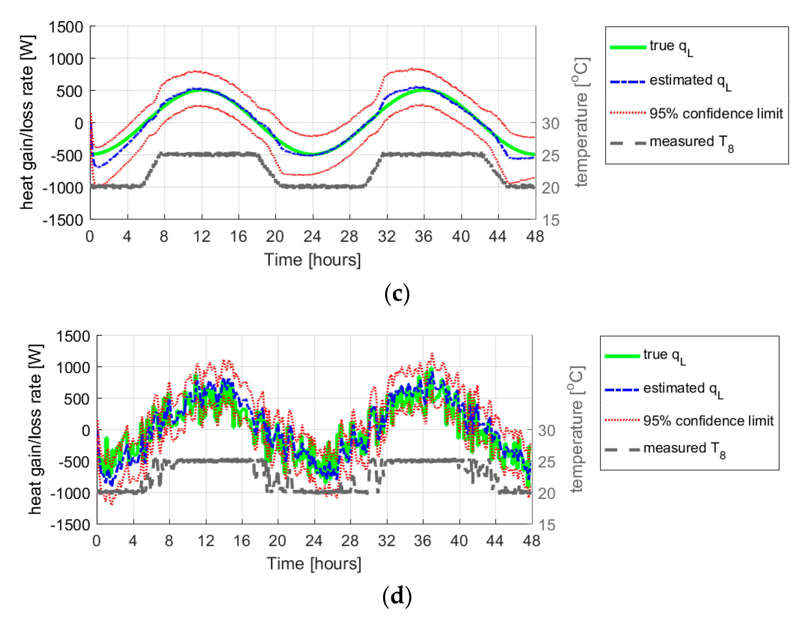
3.3. Results
4. Mini Test-Bed Experiment
4.1. Augemented State Space Model of the Mini Test-Bed
4.2. Results
5. Conclusions
Acknowledgments
Author Contributions
Conflicts of Interest
References
- American Society of Heating, Refrigerating and Air-Conditioning Engineers (ASHRAE). ASHRAE Handbook of Fundamentals; American Society of Heating, Refrigerating and Air-Conditioning Engineers, Inc.: Atlanta, GA, USA, 2013. [Google Scholar]
- McWiliams, J. Review of Airflow Measurement Techniques; LBNL-49747; Lawrence Berkeley National Laboratory: Berkeley, CA, USA, 2002.
- Hopfe, C.J.; Hensen, J.L.M. Uncertainty analysis in building performance simulation for design support. Energy Build. 2011, 43, 2798–2805. [Google Scholar] [CrossRef] [Green Version]
- Ahn, K.U.; Kim, D.W.; Kim, Y.J.; Yoon, S.H.; Park, C.S. Issues to Be Solved for Energy Simulation of An Existing Office Building. Sustainability 2016, 8, 345. [Google Scholar] [CrossRef]
- De Wilde, P. The gap between predicted and measured energy performance of buildings: A framework for investigation. Autom. Constr. 2014, 41, 40–49. [Google Scholar] [CrossRef]
- Reddy, A.T. Literature review on calibration of building energy simulation programs: Uses, problems, procedures, uncertainty, and tools. ASHRAE Trans. 2006, 112, 226–240. [Google Scholar]
- Reddy, T.A.; Maor, I.; Panjapornpon, C. Calibrating Detailed Building Energy Simulation Programs with Measured Data Part II: Application to Three Case Study Office Buildings. HVAC R Res. 2007, 13, 243–265. [Google Scholar]
- Liu, G.; Liu, M. A rapid calibration procedure and case study for simplified simulation models of commonly used HVAC systems. Build. Environ. 2011, 46, 409–420. [Google Scholar] [CrossRef]
- Raftery, P.; Keane, M.; Costa, A. Calibrating whole building energy models: Detailed case study hourly measured data. Energy Build. 2011, 43, 3666–3679. [Google Scholar] [CrossRef]
- Heo, Y.S.; Choudhary, R.; Augenbroe, G.A. Calibration of building energy models for retrofit analysis under uncertainty. Energy Build. 2012, 47, 550–560. [Google Scholar] [CrossRef]
- American Society of Heating, Refrigerating and Air-Conditioning Engineers (ASHRAE). 90.1 User’s Manual; ANSI/ASHRAE/IESNA Standard 90.1-2004; American Society of Heating, Refrigerating and Air-Conditioning Engineers, Inc.: Atlanta, GA, USA, 2004. [Google Scholar]
- Carling, P.; Isakson, P.; Blomberg, P.; Eriksson, J. Experiences from Evaluation of the HVAC Performance in the Katsan Building Based on Calibrated Whole-Building Simulation and Extensive Trending; A40-D-M6-SWE-AF/KTH-2; IEA Annex 40 Working Paper; IEA: Paris, France, 2003. [Google Scholar]
- Gelb, A. Applied Optimal Estimation; MIT Press: Cambridge MA, USA, 1974. [Google Scholar]
- Simon, D. Optimal State Estimation: Kalman, H Infinity, and Nonlinear Approaches; John Wiley & Sons: Hoboken, NJ, USA, 2006. [Google Scholar]
- Grewal, M.S.; Andrews, A.P. Kalman Filtering: Theory and Practice Using MATLAB, 2nd ed.; John Wiley & Sons, Inc.: Hoboken, NJ, USA, 2001. [Google Scholar]
- Crassidis, J.L.; Junkins, J.L. Optimal Estimation of Dynamic Systems, 2nd ed.; CRC Press: Boca Raton, FL, USA, 2011. [Google Scholar]
- Madsen, H.; Holst, J. Estimation of continuous-time models for the heat dynamics of a building. Energy Build. 1995, 22, 67–79. [Google Scholar] [CrossRef]
- Federspiel, C.C. Estimating the inputs of gas transport processes in buildings. IEEE Trans. Control Syst. Technol. 1997, 5, 480–489. [Google Scholar] [CrossRef]
- Fux, S.F.; Ashouri, A.; Benz, M.J.; Guzzella, L. EKF based self-adaptive thermal model for a passive house. Energy Build. 2014, 68, 811–817. [Google Scholar] [CrossRef]
- Ahn, K.U.; Park, C.S. Correlation between occupants and energy consumption. Energy Build. 2016, 116, 420–433. [Google Scholar] [CrossRef]
- Ahn, K.U.; Kim, D.W.; Park, C.S.; de Wilde, P. Predictability of occupant presence and performance gap in building energy simulation. Appl. Energy 2017, in press. [Google Scholar] [CrossRef]
- Yan, D.; O’Brien, W.; Hong, T.; Feng, X.; Gunay, H.B.; Tahmasebi, F.; Mahdavi, A. Occupant behavior modeling for building performance simulation: Current state and future challenges. Energy Build. 2015, 107, 264–278. [Google Scholar] [CrossRef]
- Duska, M.; Lukes, J.; Bartak, M.; Drkal, F.; Hensen, J.L.M. Trend in heat gains from office equipment. In Proceedings of the 6th International Conference on Indoor Climate of Buildings, Bratislava, Slovakia, 28 November–1 December 2007. [Google Scholar]
- Pierce, J.; Schiano, D.J.; Paulos, E. Home, habits, and energy: Examining domestic interactions and energy consumption. In Proceedings of the CHI 2010: Home Eco Behavior, Atlanta, GA, USA, 10–15 April 2010; pp. 1985–1994. [Google Scholar]
- Andrews, C.J.; Yi, D.; Krogmann, U.; Senick, J.A.; Wener, R.E. Designing buildings for real occupants: An agent-based approach. IEEE Trans. Syst. Man Cybern. Part A Syst. Hum. 2011, 41, 1077–1091. [Google Scholar] [CrossRef]
- De Wit, M.S.; Augenbroe, G.L.M. Analysis of uncertainty in building design evaluation. Energy Build. 2002, 34, 951–958. [Google Scholar] [CrossRef]
- Crawley, D.B.; Lawrie, L.K.; Winkelmann, F.C.; Buhl, W.F.; Erdem, A.E.; Pedersen, C.O.; Liesen, R.J.; Fisher, D.E. What Next for Building Energy Simulation—A Glimpse of the Future. In Proceedings of the Building Simulation ’97, Prague, Czech Republic, 7–10 September 1997; pp. 395–402. [Google Scholar]
- U.S. Department of Energy (DOE). S. Department of Energy (DOE). EnergyPlus 7.0 Engineering Reference: The Reference to EnergyPlus Calculations; U.S. Department of Energy: Washington, DC, USA, 2011.
- Mathworks. Statistics Toolbox™ User’s Guide, R2013a; MathWorks, Inc.: Natick, MA, USA, 2013. [Google Scholar]
- Fohanno, S.; Polidori, G. Modelling of natural convective heat transfer at an internal surface. Energy Build. 2006, 38, 548–553. [Google Scholar] [CrossRef]
- Yazdanian, M.; Klems, J.H. Measurement of the exterior convective film coefficient for windows in low-rise buildings. ASHRAE Trans. 1994, 100, 1087–1096. [Google Scholar]
- Alamdari, F.; Hammond, G.P. Improved data correlations for buoyancy-driven convection in rooms. Build. Serv. Eng. Res. Technol. 1983, 4, 106–112. [Google Scholar] [CrossRef]
- International Standardization Organization. ISO15099—Thermal Performance of Windows, Doors, and Shading Devices—Detailed Calculations, 1st ed.; International Standardization Organization: Geneva, Switzerland, 2003. [Google Scholar]
- Kim, D.W.; Suh, W.J.; Jung, J.T.; Yoon, S.H.; Park, C.S. A mini test-bed for modeling, simulation and calibration. In Proceedings of the Second International Conference on Building Energy and Environment, Boulder, CO, USA, 1–4 August 2012; pp. 1145–1152. [Google Scholar]


| Element | Expression |
|---|---|
| System model | |
| Measurement model | |
| Noises | Process noise: Measurement noise: * and are uncorrelated each other |
| Initial values | , |
| Prediction step | a priori error covariance calculation: Kalman gain calculation: a priori state calculation: |
| Correction step | a posteriori state calculation: a posteriori error covariance calculation: |
| Cases | Objective | Experiment Setting |
|---|---|---|
| Ref. | To test estimation performance of the KF for a time-invariant state. This can be regarded as a Reference Case. | The generated process disturbance () is set as a constant |
| #1 | To test estimation performance of the KF under sudden changes of . | The generated process disturbance () increases and decreases sharply three times a day (artificial condition). |
| #2 | To test estimation performance of the KF under smooth changes of . | The generated process disturbance () varies as a sinusoidal shape |
| #3 | To test estimation performance of the KF under random changes of . This may be close to a real-life situation in buildings (e.g., open/close windows, turn on/off lights/laptops) [20,24,25]. | Random numbers were added to the generated process disturbance () of Case #2 at every 10 min |
| List of Sensors | Sensor Noise | Unit | Reference |
|---|---|---|---|
| Outdoor air temperature | ±0.5 | (°C) | HOBO Weather station (H21-001) |
| Outdoor wind speed | ±1.2 | (m/s) | Gill inc. (WindSonic 1405) |
| Solar radiation | ±10 | (W/m2) | LI-COR (LI-200SA) |
| Indoor air temperature | ±0.5 | (°C) | General T-type thermocouple |
| Supply airflow speed | ±0.1 | (m/s) | TESTO vane probe (0635 9335) |
| Supply air temperature | ±0.5 | (°C) | General T-type thermocouple |
| Heat Transfer | State-Space Model | EnergyPlus |
|---|---|---|
| Wall cond. | ConductionFiniteDifference:simplified [28] | ConductionFiniteDifference [28] |
| Wall conv. (inside) | ASHRAE model [1] | FohannoPolidoriVerticalWall [30] |
| Wall conv. (outside) | SimpleCombined model [28] | MoWiTT [31] |
| Ceiling conv. | ASHRAE model [1] | AlamdariHammondStableHorizontal [32] |
| Floor conv. | ASHRAE model [1] | AlamdariHammondUnstableHorizontal [32] |
| Window conv. (inside) | ASHRAE model [1] | ISO15099Windows [33] |
| Window conv. (outside) | SimpleCombined model [28] | NaturalASHRAEVerticalWall [1] |
| Transmitted direct solar | All beam solar radiation entering the zone is assumed to be diffused on all surfaces | FullInteriorAndExterior: beam radiation reaches each surface in the zone by projecting the sun’s rays through the exterior windows. |
| Long-wave heat exchange (inside) | Surface radiosity balance equation | A grey interchange model based on the ScriptF [28] |
| Parameter | Symbol * | Value | Unit | Remark | ||
|---|---|---|---|---|---|---|
| State vector | Wall int./ext. temperature | (i = 1, ..., 12) | 25 | (°C) | Close to room air temperature | |
| Window temperature | 25 | (°C) | Close to room air temperature | |||
| Zone air temperature | 25 | (°C) | Room air temperature set point | |||
| Aggregated heat gain/loss rate | 0 | (W) | No heat input at initial stage | |||
| Initial error covariance matrix | (j = 1, ..., 14) | (±2)2 | (°C2) | A confidence range would be ±2 °C of the initial temperatures. | ||
| (±439 × 10%)2 | (W2) | A confidence range would be ±10% of normal condition (439 Watt); Heat releases of people, lights, and equipment are assumed to be 10 W/m2, 10.8 W/m2, and 125 W/person * 2 persons respectively. The floor area is 9 m2. | ||||
| Measurement matrix | 1 | (-) | Only zone air temperature was measured. Hence the measurement matrix is [0, 0, 0, 0, 0, 0, 0, 0, 0, 0, 0, 0, 0, 1, 0,]. | |||
| (n = 1, ..., 13, 15) | 0 | (-) | ||||
| Process noise covariance matrix | (m = 1, ..., 14) | (±0.2)2 | (°C2) | The process noise of temperatures would be ±0.2 °C. | ||
| (±439 × 10%)2 | (W2) | The estimate of the aggregated heat gain/loss rate can vary ±10% of 439 Watt per one minute. | ||||
| Measurement noise covariance matrix | (±2)2 | (°C2) | The measurement noise of the zone air temperature would be ±2 °C. | |||
| Case | RMSE (W) | NRMSE (%) | R-Square (-) |
|---|---|---|---|
| Ref. | 37.9 | ∞ | −∞ |
| #1 | 60.5 | 12.1 | 0.75 |
| #2 | 64.7 | 6.4 | 0.97 |
| #3 | 225.6 | 11.8 | 0.71 |
| Parameter | Symbol * | Value | Unit | Comments | |
|---|---|---|---|---|---|
| State vector | Wall int./ext. temperature | (i = 1, ..., 12) | 25 | (°C) | Close to room air temperature |
| Air temperature in the EPS box. | 25 | (°C) | Close to room air temperature | ||
| Heat release rate | 0 | (W) | No heat release at initial stage | ||
| Initial error covariance matrix | (j = 1, ..., 13) | (±2)2 | (°C2) | A confidence range would be ±2 °C of the initial values | |
| (±30 × 10%)2 | (W2) | The nominal heating cable power is 30 Watt at maximum. The confidence range would be 10% of the initial value. | |||
| Measurement matrix | 1 | (-) | Only box air temperature is measured. Hence the measurement matrix is [0, 0, 0, 0, 0, 0, 0, 0, 0, 0, 0, 0, 1, 0,]. | ||
| (n = 1, ..., 12, 14) | 0 | (-) | |||
| Process noise covariance matrix | (m = 1, ..., 13) | (±0.2)2 | (°C2) | The process noise of temperatures would be ±0.2 °C. | |
| (±30 × 10%)2 | (W2) | The estimate of the heat release rate can vary ±1% of 30 W per second. | |||
| Measurement noise covariance matrix | (±2)2 | (°C2) | The measurement noise would be ±2 °C | ||
© 2017 by the authors. Licensee MDPI, Basel, Switzerland. This article is an open access article distributed under the terms and conditions of the Creative Commons Attribution (CC BY) license (http://creativecommons.org/licenses/by/4.0/).
Share and Cite
Kim, D.-W.; Park, C.-S. Application of Kalman Filter for Estimating a Process Disturbance in a Building Space. Sustainability 2017, 9, 1868. https://doi.org/10.3390/su9101868
Kim D-W, Park C-S. Application of Kalman Filter for Estimating a Process Disturbance in a Building Space. Sustainability. 2017; 9(10):1868. https://doi.org/10.3390/su9101868
Chicago/Turabian StyleKim, Deuk-Woo, and Cheol-Soo Park. 2017. "Application of Kalman Filter for Estimating a Process Disturbance in a Building Space" Sustainability 9, no. 10: 1868. https://doi.org/10.3390/su9101868