How Does Energy Storage Increase the Efficiency of an Electricity Market with Integrated Wind and Solar Power Generation?—A Case Study of Korea

Abstract

In recent years, increasing requests to reduce greenhouse gas emissions have led to renewable resources rapidly replacing conventional power sources. However, the inherent variability of renewable sources reduces the reliability of power systems. Energy storage has been proposed as a viable alternative, as it can mitigate the variability of renewable energy sources and increase the efficiency of power systems by lowering peak electricity demand. In this study, we evaluate the benefits of integrating energy storage with combined wind and solar power generation in the Korean power system through using the dynamic optimization method. Realistic wind and photovoltaic solar power generation scenarios were estimated for actual sites. The results show that the wind power-based system benefitted more from energy storage than the combined wind and solar photovoltaic power-based system. This is because the high variability of wind power was reduced when it was combined with solar power. Co-optimization for energy and reserve costs was more beneficial than optimization for energy costs alone, which suggests that the reliability offered by storage is an important cost-saving factor, in addition to the reduction of energy costs by price arbitrage. Finally, the analysis was conducted under various scenarios to determine the validity of energy storage cost effectiveness.

1. Introduction

With increasing requests to reduce greenhouse gas (GHG) emissions, renewable resources have rapidly replaced conventional, non-renewable power sources in recent years. From 2000 to 2015, global nuclear power generation increased by 20 GW, while wind and solar photovoltaic power generation increased by 355 GW and 179 GW, respectively, and this trend is accelerating according to Schneider et al. [1]. Highly developed countries are leading the deployment of renewable power sources. During certain hours in 2016, Germany solely used renewable energy to meet the country’s electricity demands, and the United States and China are also actively increasing the share of renewable sources in their power sectors.

Nuclear and coal plants are the main sources of energy in South Korea, which has not actively adopted renewable sources in the power sector. Instead, the country has focused on supplying reliable and economic electricity to industry to support economic growth. Thus, solar photovoltaic and wind power only contributed 3.1% and 0.7% to generating capacity in 2015, respectively [2]. However, in 2017, increasing concerns regarding the safety of nuclear plants and air pollution from coal plants culminated in the new administration deciding to end two ongoing nuclear projects and promote the deployment of solar photovoltaic and wind power sources.

Since renewable sources such as wind and solar photovoltaic power reduce the reliability of the power system due to their inherent variability, reserve facilities that support these variable sources are necessary for stable grid operation. Energy storage has been considered as a potential solution for this. Many studies, including Walawalker et al. [3], Sioshansi [4], Hill et al. [5], Hoppman et al. [6], and Jeon et al. [7], have demonstrated that energy storage facilities can increase the efficiency of wind or solar power plants by reducing the amount of reserve energy needed by mitigating the variability of renewable sources. These papers also demonstrate that storage can reduce energy costs through enabling more renewable generation to be included in the power grid, which used to be spilled due to high variability. While energy storage used to be considered prohibitively expensive for supporting grid operation, as the cost of lithium ion batteries significantly decreases, their use in the power system is actively being reconsidered.

While many studies have discussed combining energy storage with a single renewable source, few have studied integrated wind and solar power generation with energy storage, which is more common. Studies such as Chedid et al. [8], Elhadidy [9], Nema et al. [10], and Zhou et al. [11] have assessed the impact of integrating wind and solar power generation in a small-scale system, such as a power system on an island, and replacing the existing, diesel-based power system. Integrated wind and solar systems have different characteristics to systems with a single renewable source, because in most regions, these non-dispatchable renewable sources are negatively correlated with each other since strong winds are common during the night, while solar radiation is only available during the day. Hence, integrated systems result in less variability than wind-only systems.

In this study, we conducted empirical analysis to determine the impacts of energy storage in an integrated wind and solar power system following the dynamic optimization method. Korean power system data were used, and a peak summer day was chosen for more detailed daily analysis. Realistic wind and solar photovoltaic power generation data from actual sites were estimated based on an econometric model and the Monte Carlo method.

The contributions that this study provides can be summarized as follows.

-

Firstly, it presents a dynamic optimization model that allows the impacts of variable renewable sources and energy storage to be analyzed with realistic wind and solar photovoltaic generation scenarios, estimated based on a econometric model on a national scale.

-

Secondly, this paper analyzes the impact of energy storage on a power system with integrated wind and solar sources, and provides a comparison of the benefits of using storage for wind, solar, and combined systems.

-

Thirdly, this paper analyzes the impact of energy storage under two optimization schemes by a system operator. One co-optimizes both energy and reserve costs, while the other optimizes energy costs alone. The results from the two optimization schemes can indicate how beneficial storage is when price arbitrage is the sole focus, and when both price arbitrage and variability mitigation are considered.

-

Finally, an analysis of the validity of energy storage cost effectiveness is conducted under various scenarios by comparing marginal savings in energy, reserve, and capacity components with the marginal capital costs of energy storage.

2. Model Specification

2.1. System Operator’s Optimization Model

Equations (1)–(9) is the optimization model that minimizes operation costs, which are the sum of energy and reserve costs. Equation (1) is the objective function that minimizes the sum of energy and reserve costs over a 24-h period. Net demand is the control variable, which is conventional power demand minus renewable power generation.

Equations (2) and (3) are the constraints for the hourly charging and discharging power limits of energy storage. Equation (4) is a constraint that limits the energy level of the storage device between the predetermined upper and lower bounds. In this equation, the power efficiency of the storage device (CE_t) is applied during charging and discharging. Equation (5) defines the structure of the key control variable, net demand, which system operators are responsible for satisfying.

Equation (6) shows the structure of energy costs. Energy cost is a function of net demand, and the net demand is multiplied by the temporally variable energy price. Equation (7) shows the structure of reserve costs. In this model, reserve costs consist of three components: load following, operation, and ramp wear and tear costs. The load-following reserve cost is a function of changes in net demand; hence, when net demand is highly variable due to renewable power generation, the load-following reserve cost increases. The operation reserve cost is assumed to be 3% of net demand, which is the amount that the operators of the Korean power system maintain. Ramp wear and tear costs are the result of physical stress imposed on power generators due to rapid changes in power output, which are caused by the variability of renewable generation. This cost has been discussed in recent studies, including Troy et al. [12], Kumar et al. [13], Lamadrid et al. [14], and Wogrin et al. [15]. The methodology of applying ramp wear and tear costs in this model follows Jeon [16]. The ramp wear and tear cost is proportional to net demand change.

Equation (8) shows that energy price is a function of net demand, and this function is estimated using the ordinary least squares method on historic data. In Equation (9), VRES compensates for residual energy in storage by its opportunity cost during the final optimization period.

Table 1. Nomenclature used in the model description.

Term	Description
EC	Energy cost
RC	Reserve cost
VRES	Value of residual energy in storage
ESS	Energy storage system
NGt	Net demand
Dt	Base demand
WGt	Wind power generation
PVt	Photovoltaic solar power generation
ESSt,ch	ESS charging amount
ESSt,dis	ESS discharging amount
CEt	ESS charging and discharging efficiency
EPt	Energy price
RWC()	Ramp wear cost
LRC()	Load-following reserve cost
ORC()	Operating reserve cost
PLt()	Lower limit of ESS charging and discharging constraint
PUt()	Upper limit of ESS charging and discharging constraint
ELtESS	Lower limit of energy that can be stored in the ESS
EUtESS	Upper limit of energy that can be stored in the ESS

presents detailed descriptions of the variables used in the optimization model.

Equation (1) System operator’s optimization model.

$$\underset{N{G}_t}{\min }{\displaystyle \sum }_{t=1}^{24}EC(N{G}_t)+RC(N{G}_t,\left|\mathsf{\Delta }N{G}_t\right|,{\left|\mathsf{\Delta }N{G}_t\right|}^2)-VRES$$

(1)

Subject to equation

$${\mathrm{PL}}_{\mathrm{t}}^{ch}\le ES{S}_t^{ch}\le {\mathrm{PU}}_{\mathrm{t}}^{ch},\forall t=1,\dots ,24$$

(2)

$${\mathrm{PL}}_{\mathrm{t}}^{dis}\le ES{S}_t^{dis}\le {\mathrm{PU}}_{\mathrm{t}}^{dis},\forall t=1,\dots ,24$$

(3)

$${\mathrm{EL}}_{\mathrm{t}}^{ESS}\le ES{S}_{initial}+{\displaystyle \sum }_{t=1}^{T^{\prime }}\left(C{E}_t·ES{S}_t^{ch}-\frac{1}{C{E}_t}·ES{S}_t^{dis}\right)\le E{U}_t^{ESS},\forall T^{\prime }=1,\dots ,24$$

(4)

$${\mathrm{NG}}_{\mathrm{t}}=D_t-W{G}_t-P{V}_t+ES{S}_t^{ch}-ES{S}_t^{dis}$$

(5)

$$\mathrm{EC}\left({\mathrm{NG}}_{\mathrm{t}}\right)=E{P}_t·N{G}_t$$

(6)

$$RC\left(N{G}_t\right)=LRC\left(\left|\mathsf{\Delta }N{G}_t\right|\right)+ORC\left(N{G}_t\right)+RWC({\left|\mathsf{\Delta }N{G}_t\right|}^2)$$

(7)

$${\mathrm{EP}}_{\mathrm{t}}=f\left(N{G}_t\right)$$

(8)

$$\mathrm{VRES}={\mathrm{P}}_{\mathrm{Opportunity}\mathrm{Cost}\mathrm{of}\mathrm{RES}}·RES$$

(9)

2.2. Model for Wind and Solar Photovoltaic Power Generation

Figure 1 shows the locations of the 12 largest wind and seven largest solar farms selected for this study, which account for approximately 89% and 87% of the total wind and solar photovoltaic power installations in South Korea, respectively.

Table 2. Descriptions of the selected wind farms. AWS: Automated weather station.

Site Number	Wind Farm	AWS Site Number	Capacity Allocated (MW)	Site Number	Wind Farm	AWS Site Number	Capacity Allocated (MW)
1	Hoengseong	525	634.1	7	Youngam	731	634.1
2	Pyongchang	526	1,553.5	8	Youngkwang	769	317.0
3	Taeback	878	424.8	9	Youngheung	664	285.3
4	Youngyang	801	974.9	10	Hangwon	781	908.3
5	Youngdeok	844	627.7	11	Seongsan	792	1077.9
6	Kyungju	859	266.3	12	Hanlim	779	359.8

and

Table 3. Descriptions of the selected solar photovoltaic farms.

Site Number	Solar Farm	AWS Site Number	Capacity Allocated (MW)	Site Number	Solar Farm	AWS Site Number	Capacity Allocated (MW)
1	Seoul	108	1004.3	5	Kyungnam	155	1755.7
2	Kangwon	101	988.0	6	Jeonbuk	146	3726.7
3	Chungnam	133	1239.7	7	Jeonnam	243	5462.4
4	Kyungbuk	143	2388.1	-	-	-	-

show the sites’ names, allocated generation capacities, and the AWS (Automated Weather Station from the Korea Meteorological Administration) station number for each selected site. The target capacities of wind and solar photovoltaic power that the government set for 2029 are 8064 MW and 16,565 MW, respectively. These target capacities were assigned proportionally based on the current installation capacity of each location. Hourly wind speed, solar radiation, and temperature data were collected from each corresponding AWS station.

To produce realistic wind power generation profiles, wind speed was estimated using the two-stage ARMAX model (ARIMA (Autoregressive Integrated Moving Average) with exogenous variables), as shown in Equations (10)–(12). In the first stage, which is described in detail in Equation (12), one-year, half-year, one-day, and half-day cycles, as well as cooling (CDD (Cooling degree days index = Max (temperature − 18, 0))) and heating degree days (HDD (Heating degree days index = Max (18 − temperature, 0))) were set as the main explanatory variables for wind speed, so that log(wind speed + 1) (To avoid zero wind speed in log function, one is added) could be estimated using the OLS (Ordinary Least Square). In the second stage, the ARIMA model was estimated, with the residuals (u_t) of the OLS estimation equation set as dependent variables to address autocorrelation. For the solar generation estimation model, solar radiation from seven sites was used instead of wind speed in Equation (10).

Equation (2) Two-stage ARIMA with exogenous variables (ARMAX) model for wind speed estimation.

$$\mathrm{Stage}1:\mathrm{Log}\left({\mathrm{windspeed}}_{\mathrm{it}}+1\right)={\mathrm{f}}_{\mathrm{t}}\left(DeterministicCycle{s}_t,CD{D}_t,HD{D}_t\right)+u_t$$

(10)

$$\mathrm{Stage}2:u_t:(1-{\displaystyle {\sum }_{i=1}^p}{\alpha }_i{L}^i)u_t=(1+{\displaystyle {\sum }_{i=1}^q}{\theta }_i{L}^i){ϵ}_t$$

(11)

Equation (3) Description of stage one of the ARMAX model.

$$\begin{array}{cc}\hfill \mathrm{Log}(\mathrm{wind}{\mathrm{speed}}_{\mathrm{it}}& +1)\hfill \\ & ={\beta }_{i0}+{\beta }_{i0}c{y}_t+{\beta }_{i0}s{y}_t+{\beta }_{i0}cy{h}_t+{\beta }_{i0}sy{h}_t+{\beta }_{i0}c{h}_t+{\beta }_{i0}s{h}_t\hfill \\ & +{\beta }_{i0}ch{h}_t+{\beta }_{i0}sh{h}_t+{\beta }_{i0}CD{D}_{\mathit{it}}+{\beta }_{i0}HD{D}_{\mathit{it}}+u_t\hfill \end{array}$$

(12)

where,

-

Log(wind speed_it + 1) = log transformed (wind speed + 1) at time t and location i

-

cy_t, sy_t, cyh_t, syh_t: yearly cycle (full and half year of sine and cosine curves)

-

ch_t, sh_t, chh_t, shh_t: daily cycle (full and half day of sine and cosine curves)

-

CDD_it: Cooling degree day at time t and location i

-

HDD_it: Heating degree day at time t and location i

Table 4. Estimation results of the two-stage ARMAX model at wind site two.

Stage 1: Wind Speed OLS Model			Stage 2: OLS Residual ARIMA Model
Explanatory Variable	Coefficient Estimate	t-Value	Explanatory Variable	Coefficient Estimate	t-Value
Constant term	0.66218	135.49	MU	0.00018	0.03
cy	−0.02323	−3.49	MA 1,1 (lag1)	0.36081	43.03
sy	−0.00706	−2.02	MA 1,2 (lag2)	0.05529	7.61
cyh	−0.06844	−23.21	MA 1,3 (lag3)	0.02551	3.61
syh	−0.06269	−21.36	MA 1,4 (lag4)	0.02485	3.57
ch	−0.05202	−17.72	AR 1,1 (lag1)	0.89583	159.24
sh	−0.00753	−2.75	AR 2,1 (lag24)	0.06241	10.11
chh	0.04070	15.43
shh	0.04386	16.65
CDD	0.01124	9.08
HDD	0.02323	40.92
Adjusted R2 0.2239			Pseudo R2 0.6231

shows the estimation results of the two-stage ARMAX model at wind site two. The explanatory power of the first OLS part is approximately 22.3%, and the explanatory power of the whole model is approximately 62.3%, which is adequate for a wind estimation model.

To produce realistic wind generation scenarios, we applied the Monte Carlo simulation method to the estimated two-stage ARMAX model to generate 1000 forecasted sample profiles. The white noise residuals of the ARMA part of the wind estimation model were used and randomly generated to construct the 24-h forecasting sample profiles, as shown in Figure 2. Among the 1000 sample profiles, 5%, 50%, and 95% percentile profiles were selected and converted to wind power level, and were used as wind generation inputs for optimization as low, mid, and high wind days, respectively. Figure 3a shows the 5%, 50%, and 95% percentile profiles of wind generation for a peak summer day.

The same methodology was applied to generate sample profiles for solar photovoltaic power generation. From the 1000 simulated solar generation profiles in Figure 2b, the 5%, 50%, and 95% percentile profiles were estimated and used as inputs for optimization, as shown in Figure 3b.

3. Results

3.1. Daily Optimization Result

Table 5. Descriptions of scenarios.

Scenario Name	Description
Wind-only	Korean power system + wind capacity of 8064 MW (target capacity by 2029) + energy storage of 10 GWh
Solar-only	Korean power system + solar capacity of 16,565 MW (target capacity by 2029) + energy storage of 10 GWh
Combined	Korean power system + both wind and solar capacity used above (target capacity by 2029) + energy storage of 10 GWh

describes each scenario that we studied to analyze the effect of energy storage on power systems with different renewable sources. The wind-only scenario is a basic Korean power system with a wind capacity of 8064 MW, which is the government’s target capacity by 2029. The solar-only scenario is a basic Korean power system with a solar photovoltaic capacity of 16,565 MW, and the combined scenario is a basic Korean power system with both wind and solar generation at the capacities used above. For each scenario, the effects of base and net demand were computed, and optimum demand was estimated based on optimization with 10 GWh of energy storage.

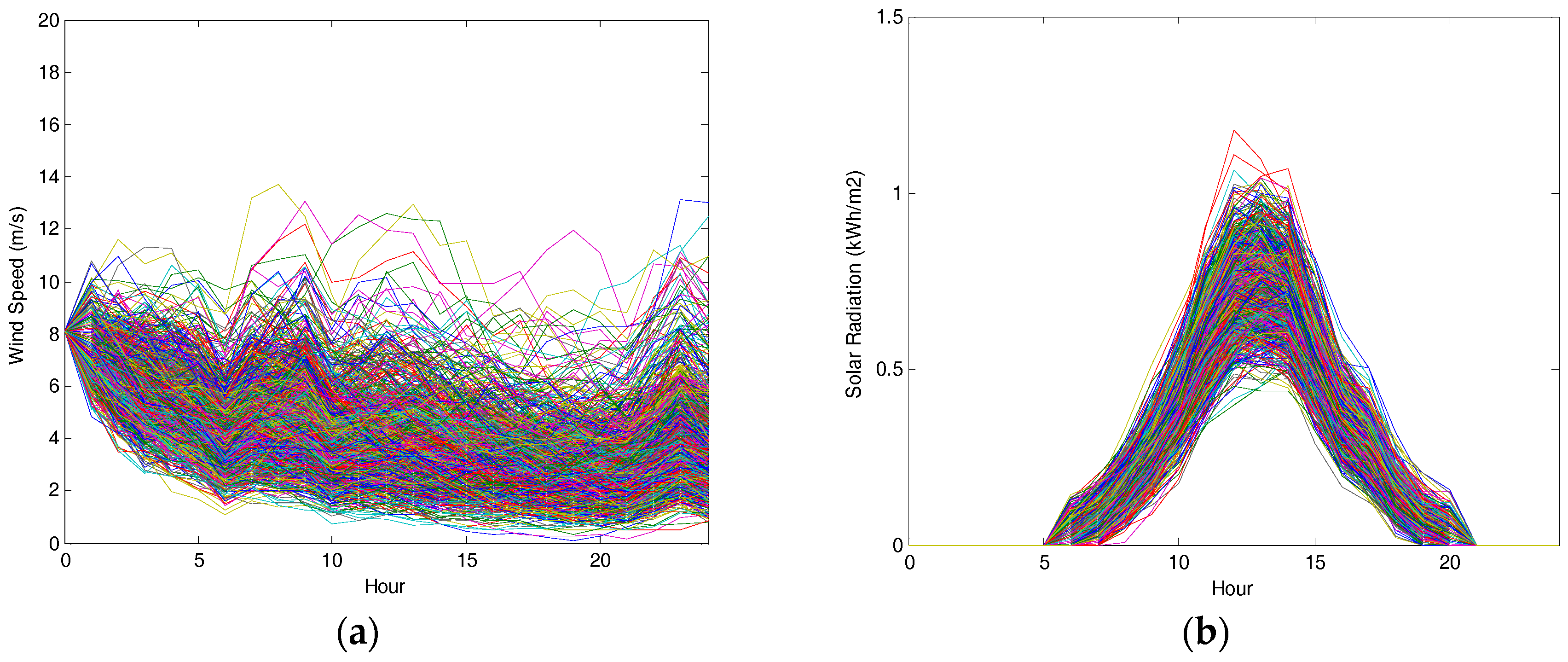
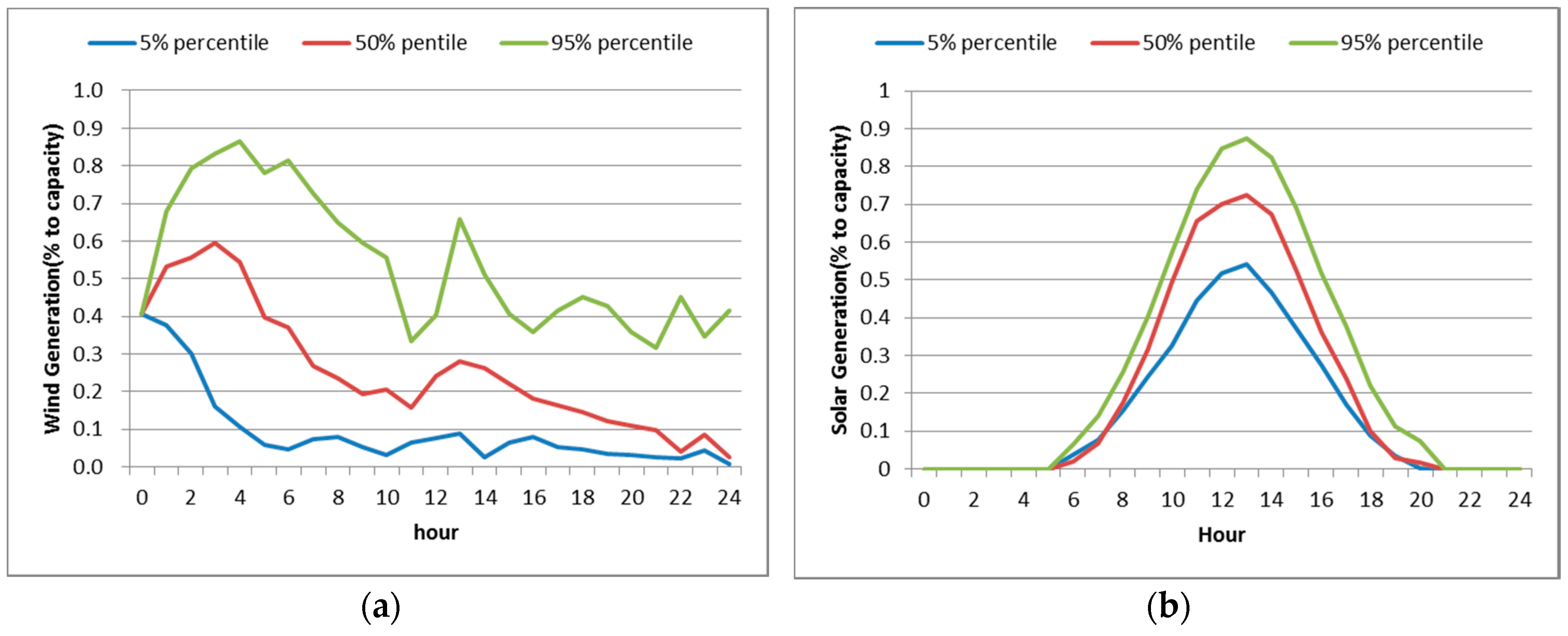
The same methodology was applied to generate sample profiles for solar photovoltaic power generation. From the 1000 simulated solar generation profiles in Figure 2b, the 5%, 50%, and 95% percentile profiles were estimated and used as inputs for optimization, as shown in Figure 3b.

For each scenario, analysis was conducted for low, mid, and high days for each renewable source, which were the 5%, 50%, and 95% percentile profiles of the simulations, respectively. The energy storage capacity was assumed to be 10 GWh. 10 GWh is chosen because it is approximately 10% of peak electricity demand of Korea, and thus can start to create some meaningful impacts on the Korean power system. Also, the target capacity of wind and solar photovoltaic power used in this study is 8064 MW and 16,565 MW, respectively. Hence, this storage capacity is approximately the size that can manage the variability caused by these renewable power sources.

The charging and discharging hourly power limits were assumed to be one-third of capacity level. The storage efficiency was assumed to be 95% for each charging and discharging cycle. The charging and discharging efficiency of a Lithium ion battery varies from 90% to 99% by its technology and specification. This paper uses 95% for efficiency based on products manufactured by KOKAM [17].

(a) Wind-Only Scenario

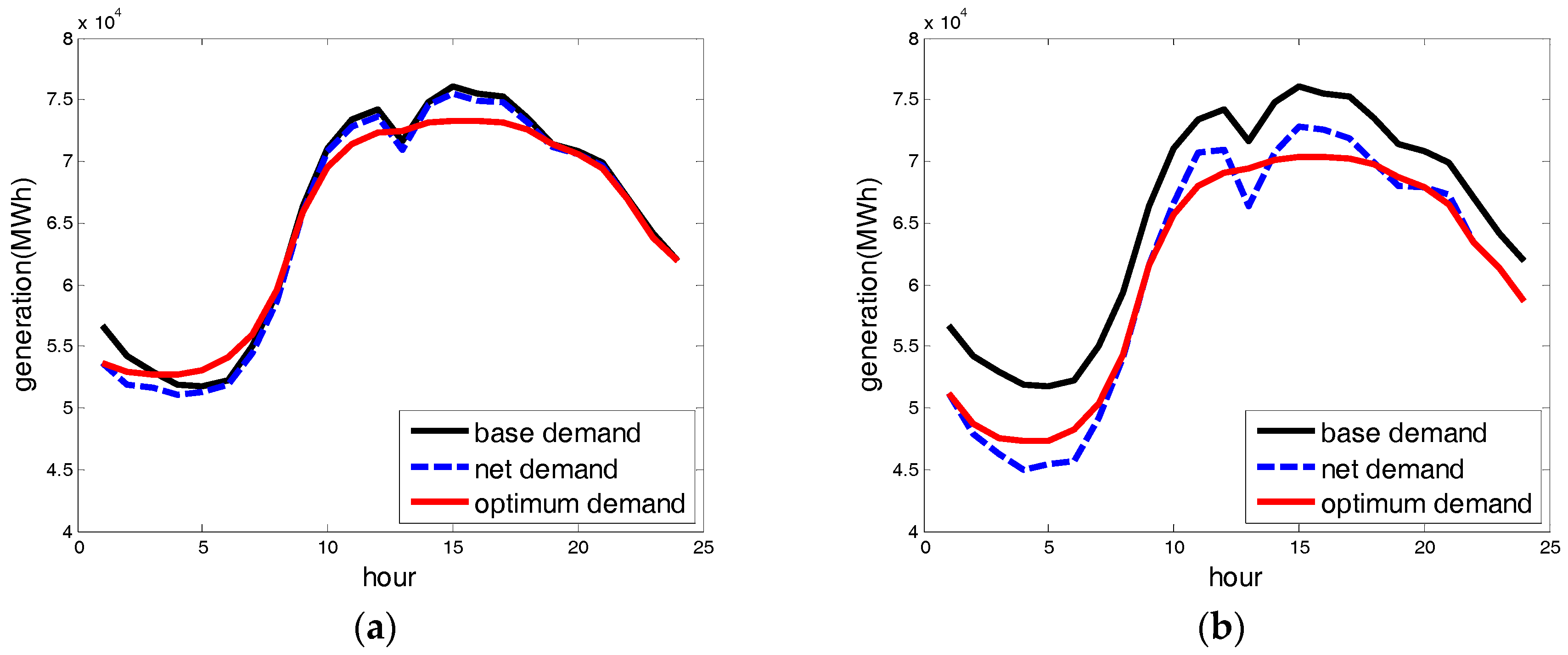
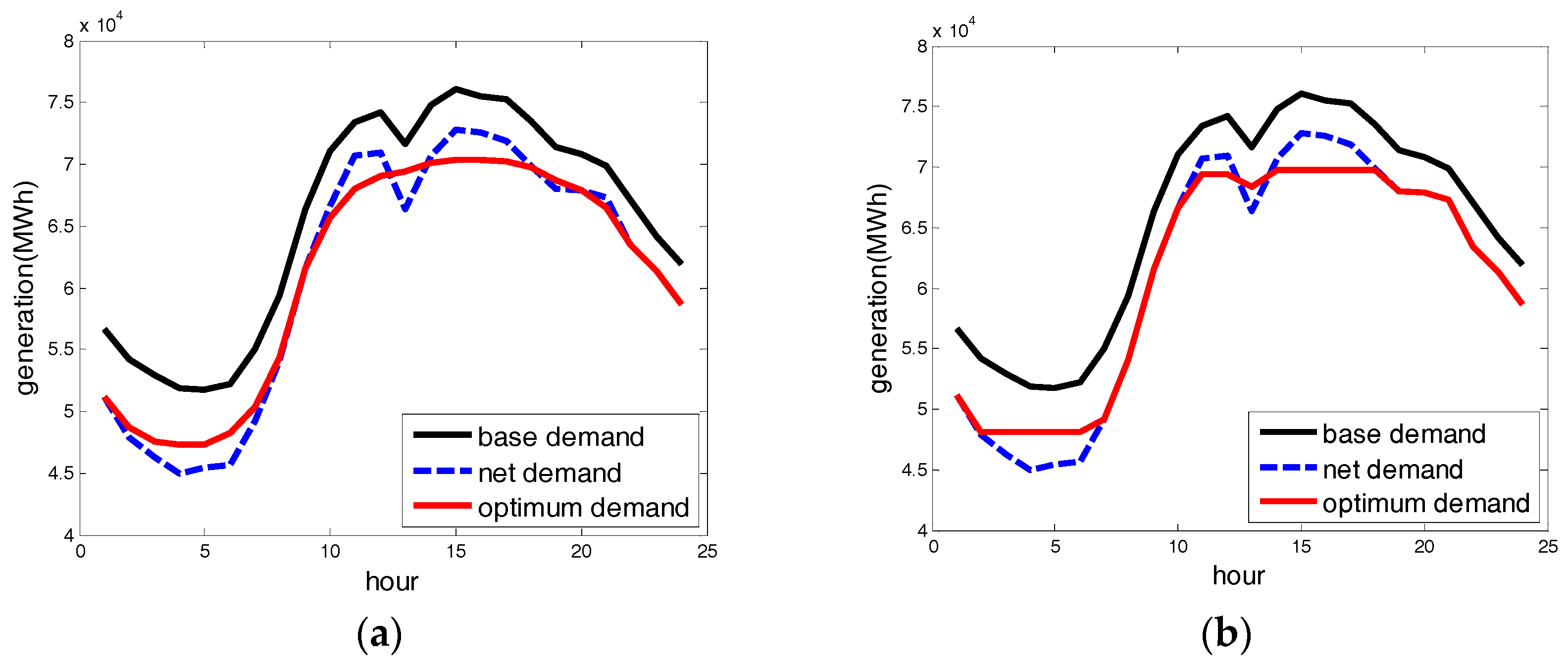
Figure 4 shows the 24-h profiles of base and optimum demand, which is net demand optimized by energy storage to minimize the energy and reserve costs on the chosen summer day. To compare high and low wind days, two sets of optimization results are presented. The optimization results show that, in both the high and low wind-only scenarios, energy storage charged during the early hours and discharged during the peak hours for price arbitrage, and it almost smoothed the net demand profiles to minimize reserve costs.

Table 6. Daily operating costs of meeting base, net, and optimum demand: wind-only scenario.

($1000/Day)	Base Demand	Low Wind-Only Scenario		High Wind-Only Scenario
		Net Demand	Optimum Demand	Net Demand	Optimum Demand
Energy Cost	146,829	144,509 (98.4%) *	144,182 (98.2%)	131,200 (89.4%)	130,810 (89.1%)
Reserve Cost	1344	1352 (100.6%)	931 (69.3%)	1766 (131.4%)	1115 (83.0%)
Operating Reserve Cost	476	474	383	563	415
Load-Following Reserve Cost	386	378	248	516	311
Ramp Wear and Tear Cost	482	480	300	687	389
Operating Cost	148,173	145,861 (98.4%)	145,113 (97.9%)	132,966 (89.7%)	131,924 (89.0%)
Peak Demand (MW)	76,054	75,540 (99.3%)	73,318 (96.4%)	72,783 (95.7%)	70,306 (92.4%)

* All figures in parenthesis show percentages compared with base demand.

presents the operation costs of base, net, and optimum demand of two of the wind-only scenarios on the peak summer day. For the high wind-only scenario, meeting net demand has significantly lower energy costs and much higher reserve costs than meeting base demand. This is because wind generation effectively replaces expensive fossil-fuel generation, but inherent variability increases the reserve costs by about 31%. Compared with net demand, the energy costs of meeting optimum demand are smaller again, as the expensive peak demand is moved to off-peak hours. Reserve costs are also significantly smaller, as energy storage effectively mitigates for the variability of wind generation. As seen in Figure 4b, net demand is smoothed by energy storage. The low wind-only scenario has similar results to the high wind-only scenario, but increases in reserve costs are limited as wind power generation is not as variable. Thus, the low wind-only scenario saves only $748,000/day in operation costs, while the high wind-only scenario saves $1,042,000/day. The peak demand of each scenario indicates how much the energy storage reduces the maximum energy required for system adequacy.

(b) Solar-only scenario

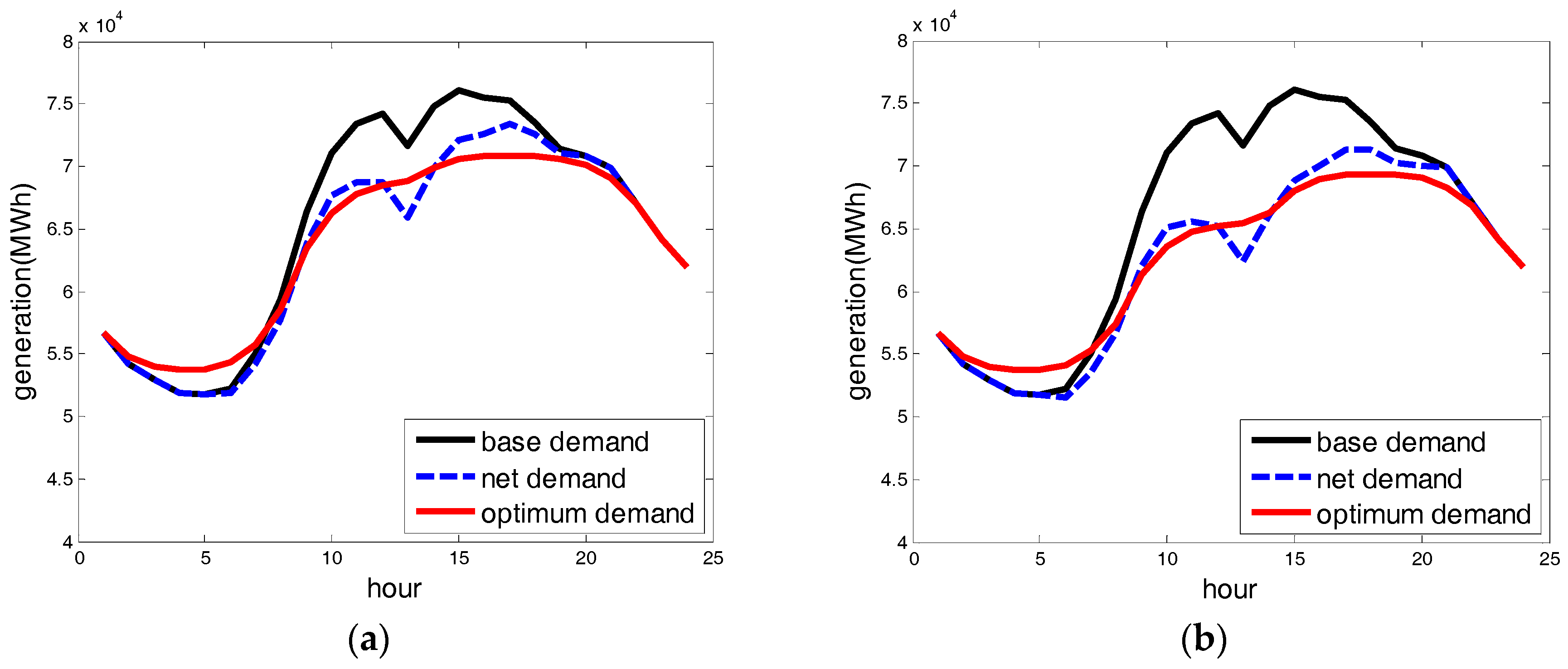
Figure 5 shows the base, net, and optimum demand of the solar-only scenario for the same summer day. The net demand of the solar-only scenario is less variable, and the difference between off-peak and peak demand is less noticeable than that of the wind-only scenario, as solar power is typically produced during peak hours. Hence, although optimum demand includes price arbitrage and demand profile smoothing, cost saving would be limited, as the price difference between peak and off-peak hours is also limited, and the net demand of the solar-only scenario is less variable than the wind-only scenario.

This is confirmed in

Table 7. Daily operating costs of meeting base, net, and optimum demand: solar-only scenario.

($1000/Day)	Base Demand	Low Solar-Only Scenario		High Solar-Only Scenario
		Net Demand	Optimum Demand	Net Demand	Optimum Demand
Energy Cost	146,829	140,230 (95.5%) *	139,958 (95.3%)	135,207 (92.1%)	134,966 (91.9%)
Reserve Cost	1344	1161 (86.4%)	733 (54.5%)	1036 (77.1%)	614 (45.7%)
Operating Reserve Cost	476	430	334	398	303
Load-Following Reserve Cost	386	331	191	294	155
Ramp Wear and Tear Cost	482	400	209	345	156
Operating Cost	148,173	141,391 (95.4%)	140,692 (95.0%)	136,243 (91.9%)	135,580 (91.5%)
Peak Demand (MW)	76,054	73,417 (96.5%)	70,796 (93.1%)	71,246 (93.7%)	69,283 (91.1%)

* All figures in parenthesis show percentages compared with base demand.

. In the high solar-only scenario, energy storage only reduces energy costs by $241,000/day, reserve costs by $422,000/day, and operating costs by $664,000/day in meeting optimum demand, while the costs of the wind-only scenario (Table 6) are reduced by $390,000/day, $652,000/day, and $1,042,000/day, respectively. This indicates that energy storage is more valuable for wind power generation than solar power generation.

(c) Combined scenario

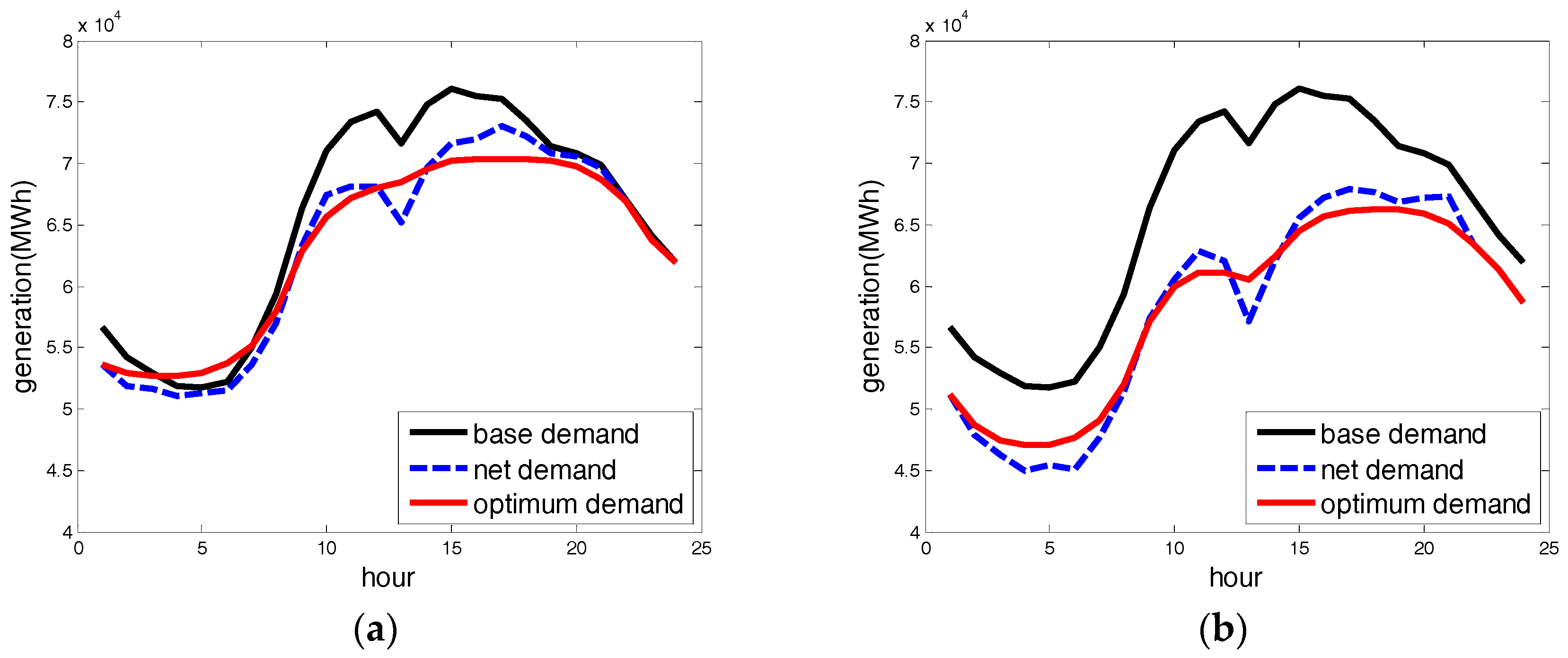
Figure 6 shows the 24-h profiles of base, net, and optimum demand of the combined scenario for the chosen summer day. The main advantage of combining wind and solar sources in a power system is that variability is reduced due to the disparity between the variability of the two sources. As seen in Figure 6, wind is more abundant during the night, while solar power is only produced during the day. Hence, when these two variable sources are combined, overall variability reduces. There is less difference between day–night demand in Figure 5b and Figure 6b.

In

Table 8. Daily operating costs of base demand, net, and optimum demand: combined scenario.

($1000/Day)	Base Demand	Low Combined Scenario		High Combined Scenario
		Net Demand	Optimum Demand	Net Demand	Optimum Demand
Energy Cost	146,829	137,949 (94.0%) *	137,674 (93.8%)	120,129 (81.8%)	119,803 (81.6%)
Reserve Cost	1344	1156 (86.0%)	706 (52.5%)	1439 (107.1%)	782 (58.2%)
Operating Reserve Cost	476	428	327	478	329
Load-Following Reserve Cost	386	325	180	424	215
Ramp Wear and Tear Cost	482	402	199	537	238
Operating Cost	148,173	139,105 (93.9%)	138,380 (93.4%)	121,568 (82.0%)	120,585 (81.4%)
Peak Demand (MW)	76,054	73,001 (96.0%)	70,399 (92.6%)	67,913 (89.3%)	66,212 (87.1%)

* All figures in parenthesis show percentages compared with base demand.

, the high combined scenario demonstrates the advantages of a combined system more clearly. The reserve cost of meeting net demand is $1,439,000/day, which is much lower than the $1,766,000/day for meeting net demand in the wind-only scenario. Energy storage in meeting optimum demand saves $326,000/day, $657,000/day, and $983,000/day of energy, reserve, and operating costs, respectively. These savings are slightly lower than those made by energy storage in the wind-only scenario. This is because the difference in day–night demand and net demand variability in the combined scenario is less severe than in the wind-only scenario. Therefore, there are fewer challenges for energy storage to mitigate for, thus there is less of a demand for it.

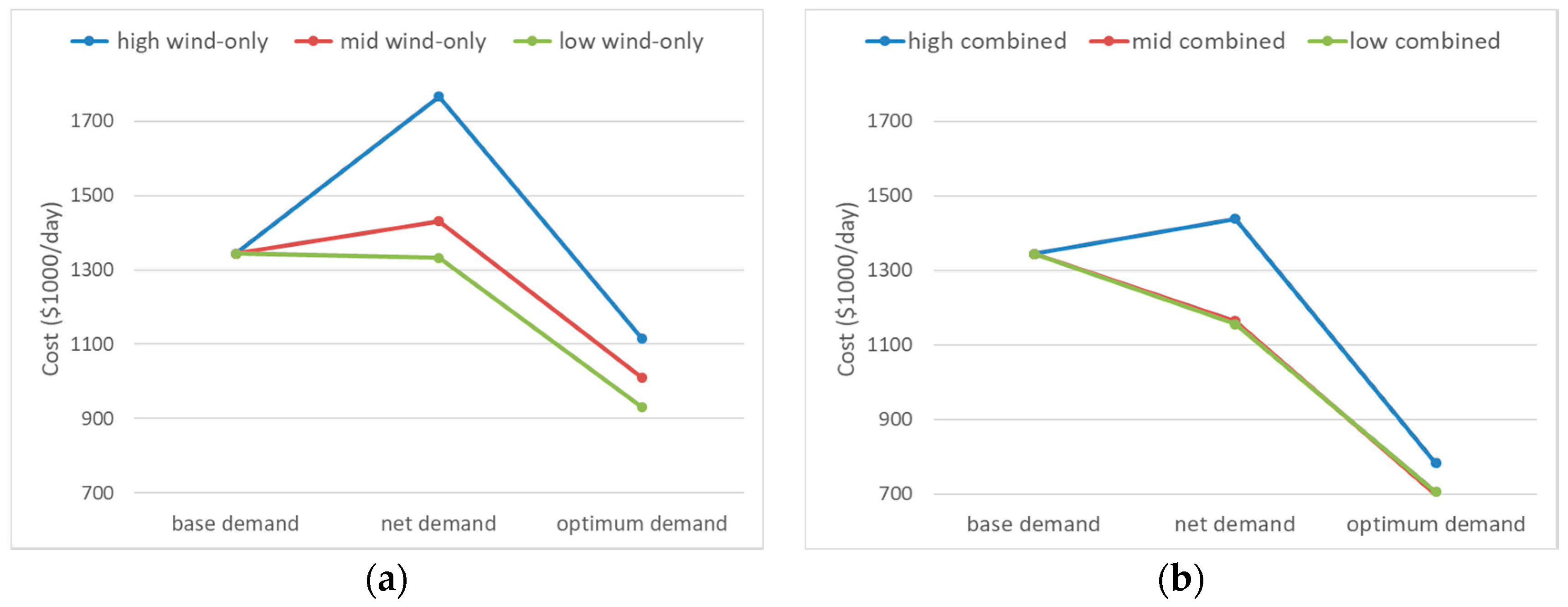
The advantages of the combined scenario over the wind-only scenario are demonstrated in Figure 7. In the wind-only scenario, the reserve costs of meeting net demand are significantly higher in the high-wind-only scenario, which is due to the variability of wind power, than when wind is combined with solar generation (Figure 7b). Figure 7b shows that a balanced installation of wind and solar power capacities in the electricity sector will benefit the operation of the power system, as it faces less variability.

3.2. Optimization with Energy Cost Alone vs. Co-Optimization with Energy and Reserve Cost

This section analyzes changes in the operation costs of the power system in scenarios when the aim of energy storage is to reduce energy costs, and when the aim is to reduce both energy and reserve costs. The value of energy storage is typically evaluated by energy cost savings from moving expensive peak demand to off-peak hours. This is not because using storage for reliability issue is less beneficial, but rather because the current rate structure under real-time pricing can compensate for price arbitrage, but not for variability mitigation. However, from the system operator’s perspective, it would be more efficient to use storage to minimize operating costs as well as energy costs. Hence, in this section, in addition to the original model for minimizing operating costs, we provide the optimization result from minimizing energy costs alone, which is what demand-side storage companies do, and compare how the efficiency of the power system varies under two different optimization schemes.

Figure 8 shows the difference between optimum demand when it is co-optimized with both energy and reserve costs, and optimum demand when it is only optimized with energy costs in the high wind-only scenario. As noted in Equation (1-1), the system operator minimizes operating costs, which are the sum of energy and reserve costs. However, energy storage is often used solely for reducing energy costs by moving expensive peak demand to off-peak hours, and this price arbitrage benefit was the most valuable factor of energy storage. Figure 8b shows the optimum demand under the optimization scheme that solely reduces energy costs. As expected, it moves as many demand peaks as possible to off-peak hours. Thus, optimum demand has several kinks that create additional costs to the system, while the optimum demand of Figure 8a is smooth.

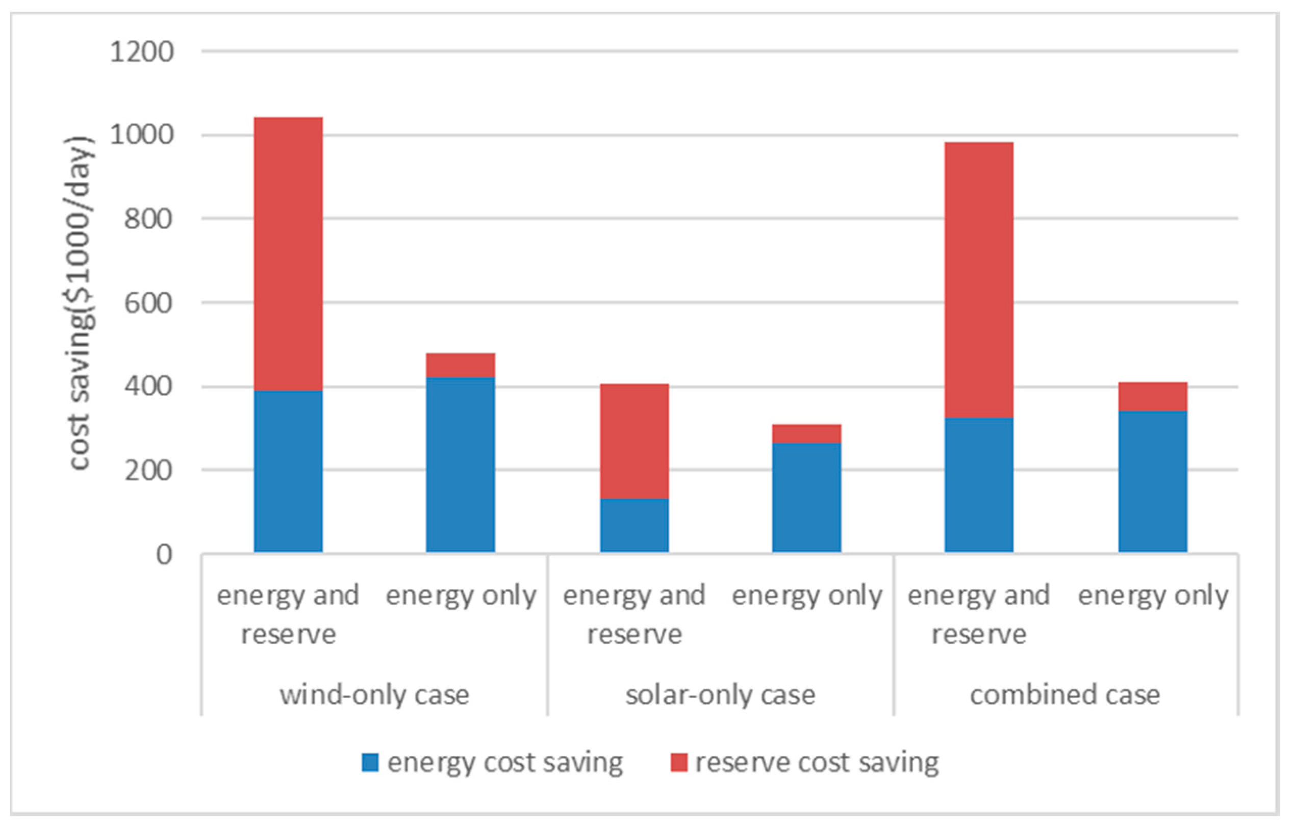
Figure 9 shows the amount of energy and reserve costs saved for each scenario when they are co-optimized for both energy and reserve costs, and optimized for energy costs alone. In all three scenarios, energy storage saves reserve costs by as much as or larger than energy costs alone when energy and reserve costs are co-optimized, whereas when energy costs are optimized alone, energy cost savings increase very marginally, and there is almost no saving of reserve costs. Energy cost savings increase very little, even when the system operator’s optimization focuses on reducing energy costs, because the benefit of arbitrage becomes saturated when more storage is used for this purpose, due to the reduction of the price difference between peak and off-peak periods. Another reason for this is storage charging/discharging inefficiency, which further reduces the price difference between peak and off-peak periods. For these reasons, allocating energy storage to reduce both energy and reserve costs is more economically viable.

3.3. Annual Cost Savings of Energy Storage

Table 9. Annual operating costs and peak demand observed for the base, net, and optimum demand of the three scenarios.

($Mil/Year)	Base Demand	Wind-Only Scenario		Solar-Only Scenario		Combined Scenario
		Net Demand	Optimum Demand	Net Demand	Optimum Demand	Net Demand	Optimum Demand
Energy cost	40,194	33,972	33,422	37,506	37,277	32,008	31,685
Reserve cost	402	587	362	287	208	436	234
Operating cost	40,597	34,558	33,784	37,794	37,486	32,444	31,920
Peak demand (MW)	76,092	72,812	70,356	71,325	70,175	67,960	66,272

shows the annual operating costs and peak demand for the base, net, and optimum demand of the three scenarios. To estimate annual costs, three representative days of each season were selected and the Piecewise Cubic Hermite Interpolating Polynomial (PCHIP) interpolation method was followed to estimate annual costs, with peak demand as the highest demand observed on the chosen representative days. The result shows that reserve costs are increased significantly for meeting the net demand of the wind-only scenario, while reserve and energy costs for meeting optimum demand are effectively reduced. In the combined scenario, the reserve cost of meeting net demand is lower than that of the wind-only scenario, indicating that the combined scenario faces less variability in net demand, as there is disparity between wind and solar power generation. Again, there are effective savings in both the reserve and energy costs of meeting optimum demand in the combined scenario.

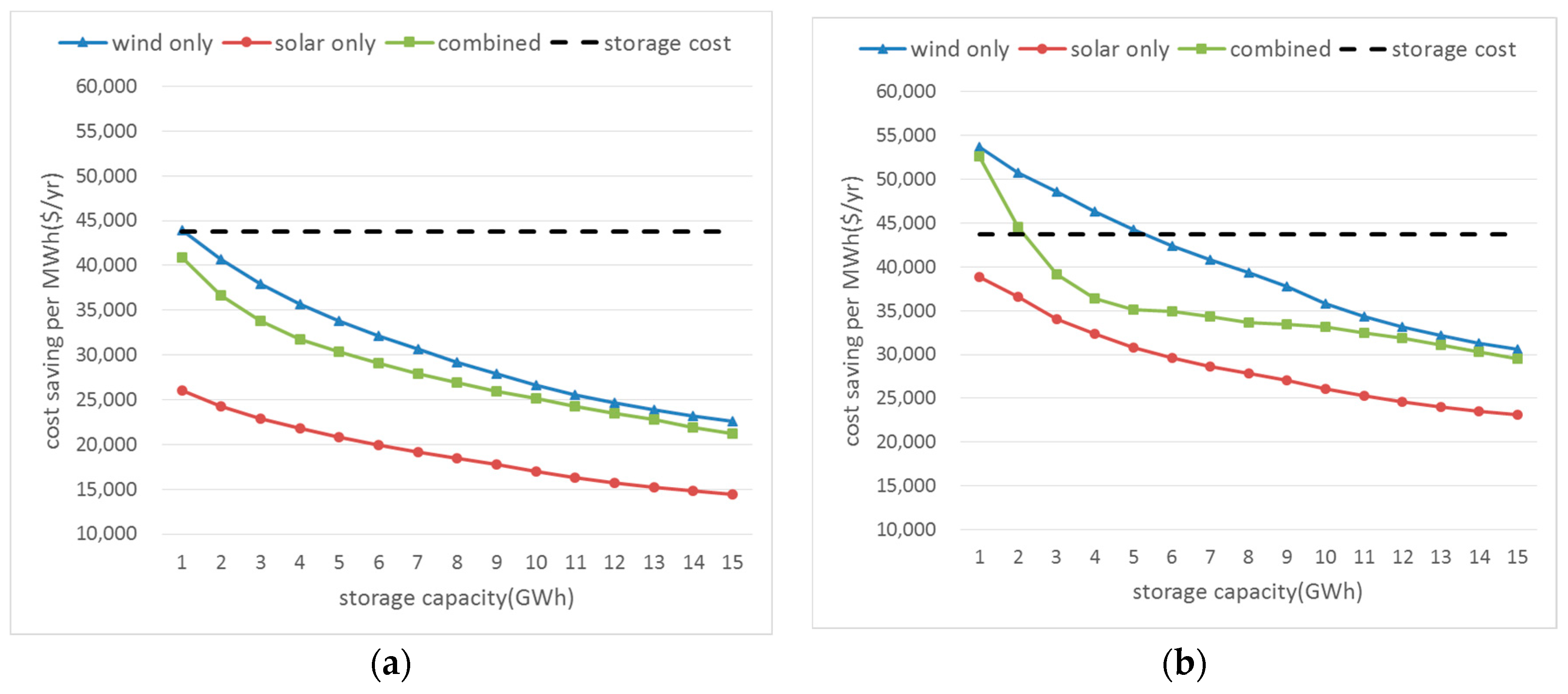
Figure 10 shows the annual costs saved per MWh of energy storage with varying storage capacities for the wind-only, solar-only, and combined scenarios and

Table 10. Annual cost savings per unit storage with varying storage sizes in a combined scenario.

($Mil/Year-MWh)	1 GWh	2 GWh	3 GWh	4 GWh	5 GWh	6 GWh	7 GWh
Energy Cost Saving	8100	8655	8946	9223	9066	8904	8748
Reserve Cost Saving	32,816	27,975	24,898	22,524	21,269	20,148	19,174
Capacity Cost Saving	11,713	7934	5290	4668	4806	5911	6366
System Cost Saving	52,630	44,564	39,134	36,416	35,140	34,962	34,288
	8 GWh	9 GWh	10 GWh	11 GWh	12 GWh	13 GWh	14 GWh
Energy Cost Saving	8607	8467	8321	8176	8034	7889	7823
Reserve Cost Saving	18,300	17,505	16,785	16,115	15,484	14,863	14,124
Capacity Cost Saving	6765	7457	8008	8178	8323	8362	8339
System Cost Saving	33,671	33,429	33,113	32,469	31,840	31,114	30,287

presents composition of annual system cost savings with varying storage capacities for the combined scenario. Figure 10a shows cost savings when operating costs were considered alone. The annual costs saved per MWh of storage decrease as storage capacity increases, because when storage size increases, the effect of reducing energy and reserve costs per unit MWh becomes less significant. The black dashed line shows the annual capital cost of storage per MWh, which is $43,750/MWh/year (based on the cost of a lithium battery cell: $350/kWh, life cycle: 10 years, PCS (Power Control System) cost and degrading cost). The annual storage cost provides a reference level for evaluating the cost effectiveness of energy storage for grid operation.

As shown in Figure 10, storage is most valuable for the wind-only scenario, followed by the combined scenario, and the solar-only scenario benefits very little from storage, as there is little variability that storage can mitigate for. As discussed above, wind power is highly variable and abundant during the night, which makes the price difference between day and night larger; therefore, it provides a better opportunity for arbitrage and a chance to reduce high reserve costs. With the current costs of storage, storage in the wind-only scenario just achieved economic viability, while in the other scenarios, the benefit is below the cost of storage.

Figure 10b shows the annual system cost savings per unit MWh of storage, which is the operating cost saving plus capacity cost saving. Capacity cost-saving was computed based on the contribution of storage to reducing peak demand, as reported in Table 8. The annual capacity cost of a gas turbine plant, $53,200/MW/year (EIA [18]) was used when computing the capacity cost saving by storage through reducing peak demand. When capacity cost reduction by storage is considered, in addition to operating cost reduction, cost savings by storage exceed costs in the wind-only and combined cases. This means that energy storage is already economic viable when its contribution to grid operation is correctly evaluated, and properly compensated at the current storage cost levels.

4. Discussion and Conclusions

This study examined how combining wind and solar sources in a power system affected operating costs compared with wind-only or solar-only systems. It also demonstrates the benefits of installing energy storage, which can be changed depending on the type of renewable source and the optimization scheme that the system operator adopts.

Due to the inherent variability of renewable sources, an increase of renewable generation in the electricity sector often leads to higher reliability costs. When two disparate renewable sources, such as wind and solar, are deployed in the same system, as in South Korea, the overall variability that the system needs to manage is decreased. This reduces the reserve costs required to maintain a reliable system.

The reserve cost of the high wind-only scenario compared with the base case was $422,000/day higher than the base scenario, whereas the reserve cost in the high combined scenario increased by only $85,000/day. This demonstrates that the variability of wind generation is decreased effectively when it is combined with solar generation. However, energy storage saved $983,000/day and $1,042,000/day in operating costs in the high combined and high wind-only scenarios, respectively. This is because, in the high wind-only scenario, energy storage can effectively reduce wind variability; thus, it can significantly reduce reserve costs. However, in the high combined scenario, wind variability is partially reduced by solar generation; thus, the effect of storage is reduced. In the high solar-only scenario, only $664,000/day of operating costs were saved by energy storage, as energy cost savings are reduced by peak reduction, which is a main characteristic of solar generation.

While storage can be effective in mitigating the variability of renewable sources, the economic value of storage is mostly due to the amount of energy costs saved by arbitrage benefit. To compare the benefits of storage when the focus is on saving energy costs alone versus saving both energy and reserve costs, this study analyzed situations where storage is operated to minimize both energy and reserve costs, and where it is operated to solely minimize energy costs. The result of this shows that operating cost savings are much higher when storage is operated to minimize both energy and reserve costs. When storage is operated to solely minimize energy costs, the energy cost savings marginally increase, but reserve cost savings significantly decrease.

The wind-only scenario had the largest savings in annual operating costs, but the marginal operating costs saved per unit MWh of storage were below the capital costs of storage in all three scenarios. However, when capacity cost savings are properly considered, the cost-saving effect of storage surpasses capital costs in the wind-only and combined scenarios.

The main outcome of this paper can be applied to other potential demand-side storages such as electric vehicle and thermal storage. With rapidly decreasing lithium battery prices, electric vehicles have become a major alternative to gasoline vehicles. The massive deployment of electric vehicles can make the electric vehicle a valuable resource to support the grid, with high renewable generation using vehicle-to-grid (V2G) technology. Load-serving entities can aggregate storage capacities from these electric vehicles while they are parked at home or work, and provide a similar service to supply-side storage to the power grid. Especially, the cost of the battery in the electric vehicle can be shared between providing its own service, which is commuting, and supporting the grid. In this way, the electric vehicle can be a more economically viable option when it can receive compensation for providing the services to the grid that this paper suggests.

Thermal storage can also provide services such as supply-side storage at a lower cost. Thermal storage works stores ice during the nighttime when electricity is cheap, and provides a cooling service mostly during the daytime, when electricity is expensive. Instead of storing electricity, it stores ice, so the capital cost of facility is much lower compared with a lithium ion battery, but it can provide almost the same service as a lithium ion battery by replacing the electricity consumed for cooling with an actual cooling service. By mitigating the cooling electricity demand required to support the grid with high renewable generation, it can contribute to not only lower energy costs, but also lower reserve and capacity costs as well.

The rapid introduction of renewable resources and decreasing capital costs make energy storage a viable option in the power system. However, the deployment of storage is still slow, because its contribution to the power system has not been properly compensated. When suitable compensation mechanisms pay each market player for the contribution they make to energy, reserve, and capacity costs, we will be able to establish a sustainable and efficient electricity market.