Impact of Urban Climate Landscape Patterns on Land Surface Temperature in Wuhan, China


Abstract
:1. Introduction
2. Materials
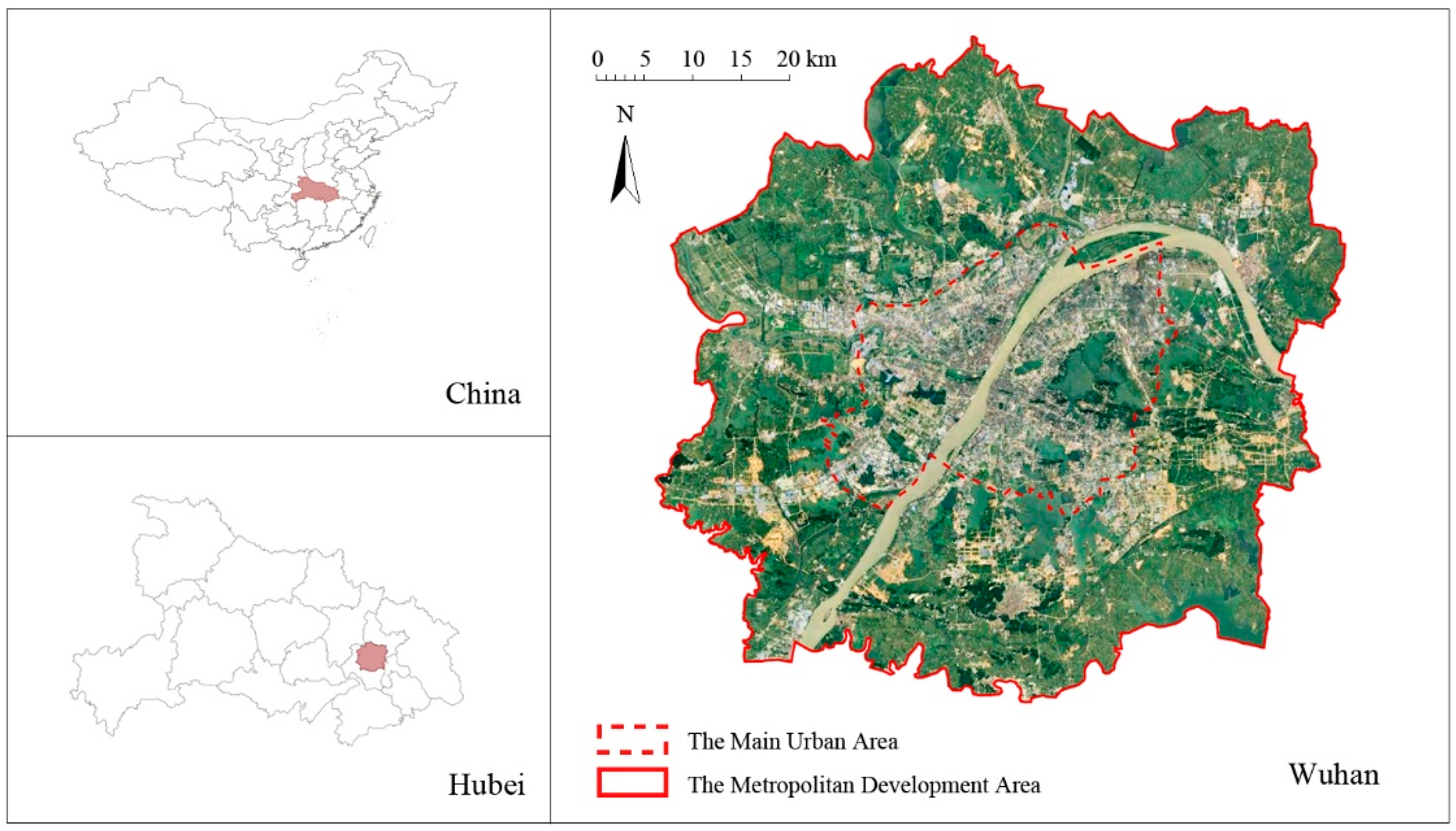
2.1. Study Area
2.2. Data Pre-Processing
3. Methodology
3.1. LCZ Classification and Validation
3.1.1. Mapping Local Climate Zones
3.1.2. Validation by LST Variation
3.2. Comparison of Different Landscapes
3.2.1. Urban Climate Landscape Pattern
3.2.2. Searching for the Optimal Scale
3.2.3. Comparison of the Pattern-Temperature Relationship
3.3. Quantification of the Heating/Cooling Effect
3.3.1. Defining the Heating/Cooling Intensity
3.3.2. Quantifying the Effect by Patch Metrics
4. Results and Discussion
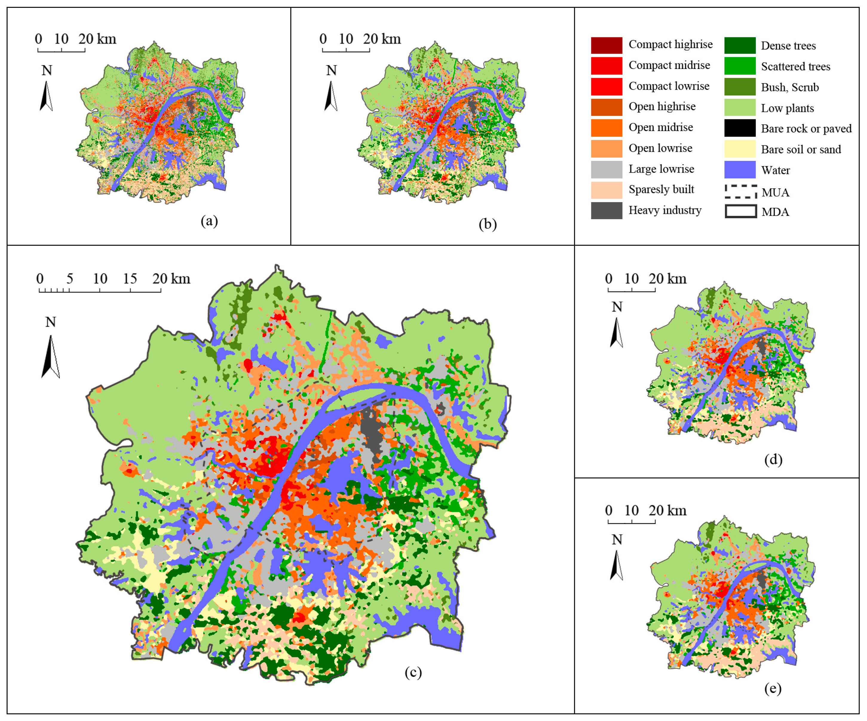
4.1. LCZ Map of Wuhan
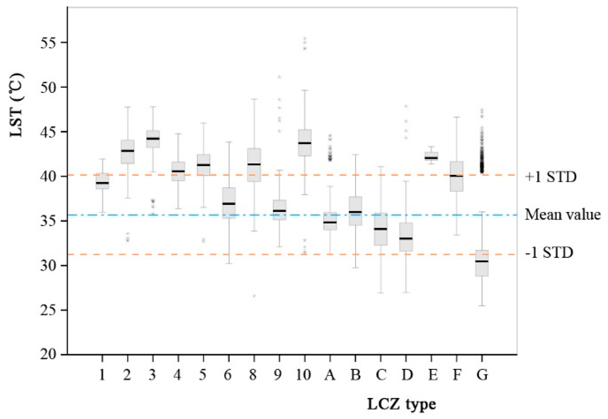
4.2. Verifying LCZs by LST Variation
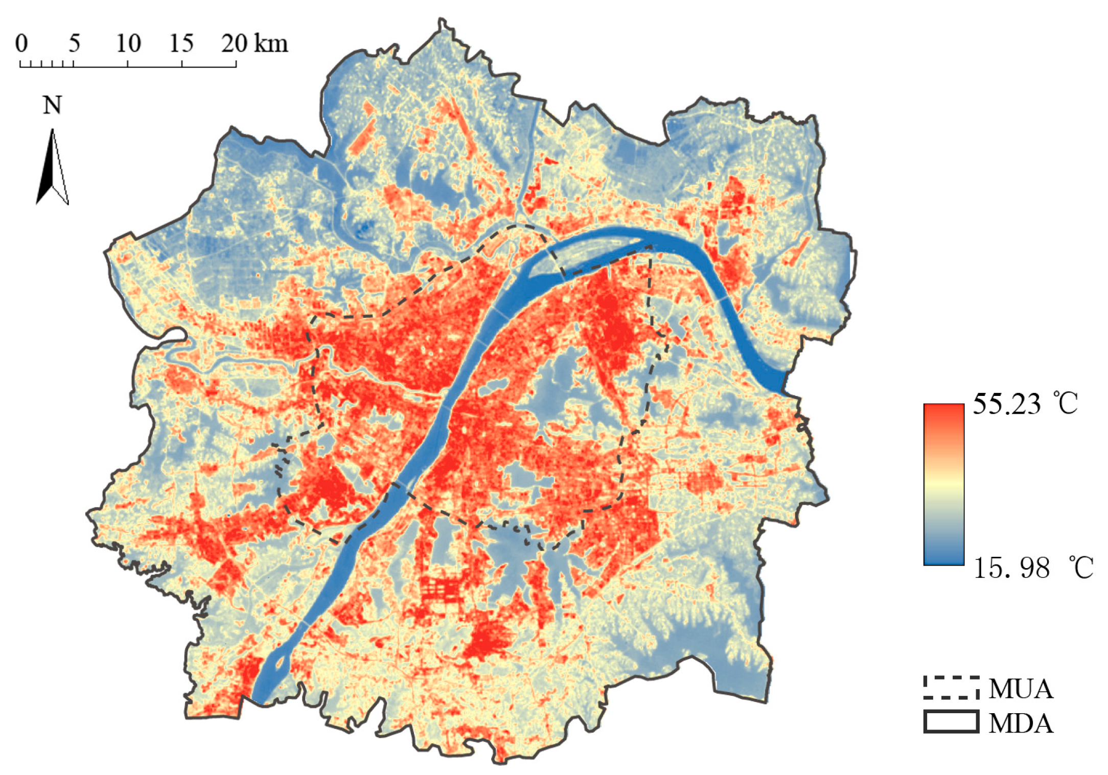
4.2.1. Distribution of LST
4.2.2. Validation of LCZ Classification
4.3. Spatial Distribution of Urban Climate Landscape and Focal Landscapes
4.3.1. Area Proportion of Each Climate Landscape
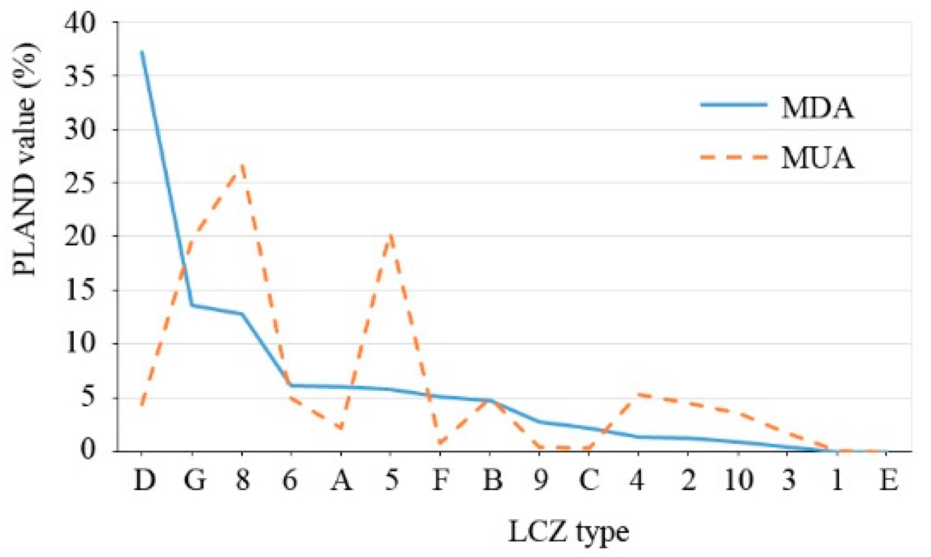
4.3.2. Selection of Focal Climate Landscapes
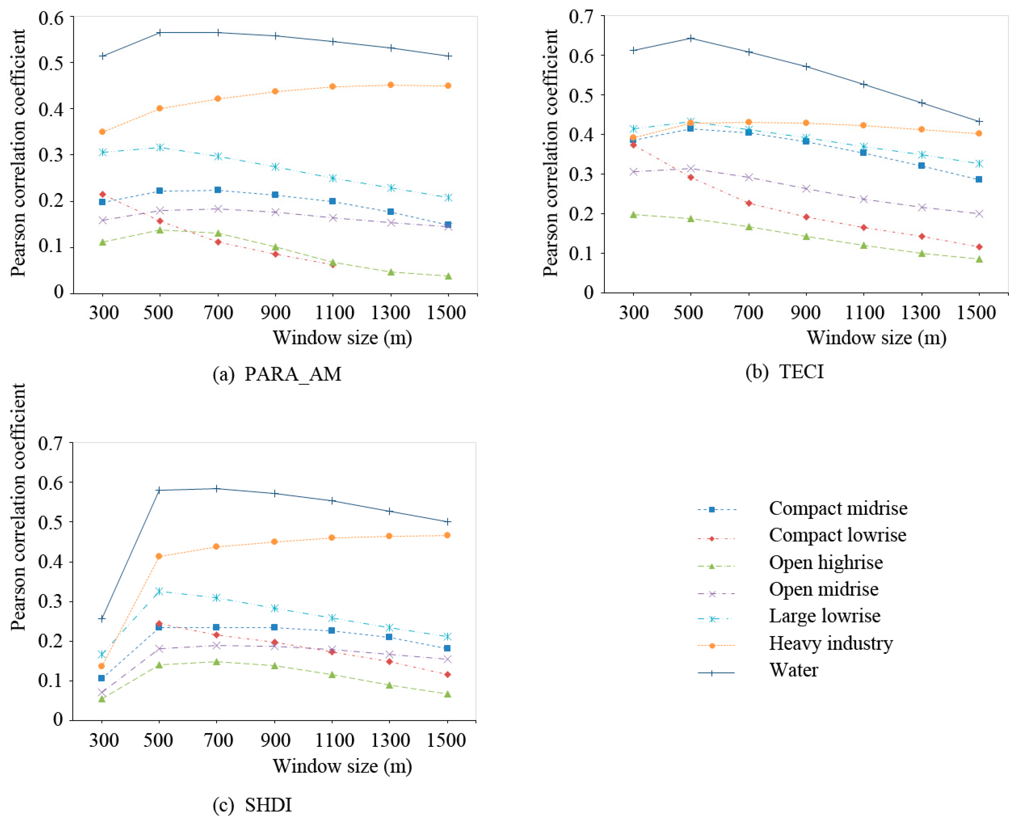
4.4. Optimal Scale for Studying Pattern-Temperature Interactions
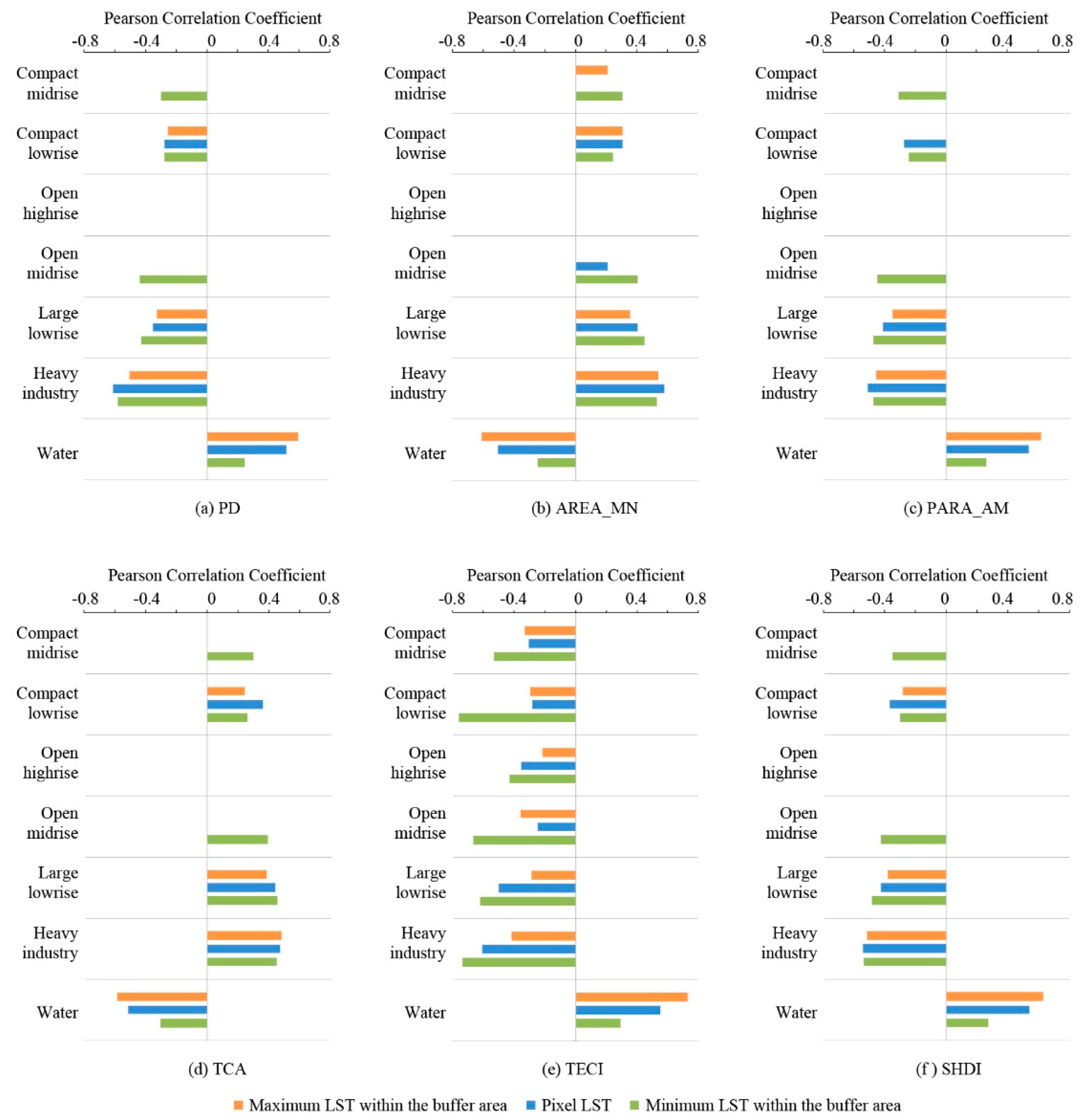
4.5. Relationship between Landscape Metrics and LST at a Fixed Scale
4.6. Impact of Patch Metrics on LST
5. Implications and Conclusions
Acknowledgments
Author Contributions
Conflicts of Interest
References
- Hoag, H. How cities can beat the heat: Rising temperatures are threatening urban areas, but efforts to cool them may not work as planned. Nature 2015, 524, 402–405. [Google Scholar] [CrossRef] [PubMed]
- IPCC. Climate Change 2014: Synthesis Report. Contribution of Working Groups I, II and III to the Fifth Assessment Report of the Intergovernmental Panel on Climate Change; IPCC: Cambridge, UK, 2014. [Google Scholar]
- Grimmond, C.S.B.; Roth, M.; Oke, T.R.; Au, Y.C.; Best, M.; Betts, R.; Carmichael, G.; Cleugh, H.; Dabberdt, W.; Emmanuel, R. Climate and more sustainable cities: Climate information for improved planning and management of cities. Procedia Environ. Sci. 2010, 1, 247–274. [Google Scholar] [CrossRef]
- Adolphe, L. A simplified model of urban morphology: Application to an analysis of the environmental performance of cities. Environ. Plan. B Plan. Des. 2001, 28, 183–200. [Google Scholar] [CrossRef]
- Unger, J. Intra-urban relationship between surface geometry and urban heat island: Review and new approach. Clim. Res. 2004, 27, 253–264. [Google Scholar] [CrossRef]
- Zhao, C.; Fu, G.; Liu, X.; Fu, F. Urban planning indicators, morphology and climate indicators: A case study for a north-south transect of beijing, China. Build. Environ. 2011, 46, 1174–1183. [Google Scholar] [CrossRef]
- Voogt, J.A.; Oke, T.R. Thermal remote sensing of urban climates. Remote Sens. Environ. 2003, 86, 370–384. [Google Scholar] [CrossRef]
- Song, J.; Du, S.; Feng, X.; Guo, L. The relationships between landscape compositions and land surface temperature: Quantifying their resolution sensitivity with spatial regression models. Landsc. Urban Plan. 2014, 123, 145–157. [Google Scholar] [CrossRef]
- Wang, J.; Zhan, Q.; Guo, H.; Jin, Z. Characterizing the spatial dynamics of land surface temperature-impervious surface fraction relationship. Int. J. Appl. Earth Obs. Geoinf. 2016, 45, 55–65. [Google Scholar] [CrossRef]
- Myint, S.W.; Zheng, B.; Talen, E.; Fan, C.; Kaplan, S.; Middel, A.; Smith, M.; Huang, H.P.; Brazel, A. Does the spatial arrangement of urban landscape matter? Examples of urban warming and cooling in phoenix and las vegas. Ecosyst. Health Sustain. 2015, 1, 15. [Google Scholar]
- Cao, X.; Onishi, A.; Chen, J.; Imura, H. Quantifying the cool island intensity of urban parks using aster and ikonos data. Landsc. Urban Plan. 2010, 96, 224–231. [Google Scholar] [CrossRef]
- Li, J.; Song, C.; Cao, L.; Zhu, F.; Meng, X.; Wu, J. Impacts of landscape structure on surface urban heat islands: A case study of shanghai, china. Remote Sens. Environ. 2011, 115, 3249–3263. [Google Scholar] [CrossRef]
- Kong, F.; Yin, H.; Wang, C.; Cavan, G.; James, P. A satellite image-based analysis of factors contributing to the green-space cool island intensity on a city scale. Urban Green. 2014, 13, 846–853. [Google Scholar] [CrossRef]
- Feng, X.; Myint, S.W. Exploring the effect of neighboring land cover pattern on land surface temperature of central building objects. Build. Environ. 2016, 95, 346–354. [Google Scholar] [CrossRef]
- Matthews, T.; Lo, A.Y.; Byrne, J.A. Reconceptualizing green infrastructure for climate change adaptation: Barriers to adoption and drivers for uptake by spatial planners. Landsc. Urban Plan. 2015, 138, 155–163. [Google Scholar] [CrossRef]
- Emmanuel, R.; Loconsole, A. Green infrastructure as an adaptation approach to tackling urban overheating in the glasgow clyde valley region, UK. Landsc. Urban Plan. 2015, 138, 71–86. [Google Scholar] [CrossRef]
- Jim, C.Y.; Chan, M.W.H. Urban greenspace delivery in hong kong: Spatial-institutional limitations and solutions. Urban Green. 2016, 18, 65–85. [Google Scholar] [CrossRef]
- Demuzere, M.; Orru, K.; Heidrich, O.; Olazabal, E.; Geneletti, D.; Orru, H.; Bhave, A.; Mittal, N.; Feliu, E.; Faehnle, M. Mitigating and adapting to climate change: Multi-functional and multi-scale assessment of green urban infrastructure. J. Environ. Manag. 2014, 146, 107–115. [Google Scholar] [CrossRef] [PubMed]
- Yuan, C.; Ng, E. Building porosity for better urban ventilation in high-density cities—A computational parametric study. Build. Environ. 2012, 50, 176–189. [Google Scholar] [CrossRef]
- Gál, T.; Unger, J. Detection of ventilation paths using high-resolution roughness parameter mapping in a large urban area. Build. Environ. 2009, 44, 198–206. [Google Scholar] [CrossRef]
- Karlessi, T.; Santamouris, M.; Synnefa, A.; Assimakopoulos, D.; Didaskalopoulos, P.; Apostolakis, K. Development and testing of pcm doped cool colored coatings to mitigate urban heat island and cool buildings. Build. Environ. 2011, 46, 570–576. [Google Scholar] [CrossRef]
- Larsen, L. Urban climate and adaptation strategies. Front. Ecol. Environ. 2015, 13, 486–492. [Google Scholar] [CrossRef]
- Stewart, I.D.; Oke, T.R. Local climate zones for urban temperature studies. Bull. Am. Meteorol. Soc. 2012, 93, 1879–1900. [Google Scholar] [CrossRef]
- Wang, J.; Ouyang, W. Attenuating the surface urban heat island within the local thermal zones through land surface modification. J. Environ. Manag. 2017, 187, 239–252. [Google Scholar] [CrossRef] [PubMed]
- Geletič, J.; Lehnert, M.; Dobrovolný, P. Land surface temperature differences within local climate zones, based on two central european cities. Remote Sens. 2016, 8, 788. [Google Scholar] [CrossRef]
- Bechtel, B.; See, L.; Mills, G.; Foley, M. Classification of local climate zones using sar and multispectral data in an arid environment. IEEE J. Sel. Top. Appl. Earth Obs. Remote Sens. 2016, 9, 3097–3105. [Google Scholar] [CrossRef]
- Danylo, O.; See, L.; Bechtel, B.; Schepaschenko, D.; Fritz, S. Contributing to wudapt: A local climate zone classification of two cities in ukraine. IEEE J. Sel. Top. Appl. Earth Obs. Remote Sens. 2016, 9, 1841–1853. [Google Scholar] [CrossRef]
- Xu, Y.; Ren, C.; Cai, M.; Edward, N.Y.Y.; Wu, T. Classification of local climate zones using aster and landsat data for high-density cities. IEEE J. Sel. Top. Appl. Earth Obs. Remote Sens. 2017, 10, 3397–3405. [Google Scholar] [CrossRef]
- Leconte, F.; Bouyer, J.; Claverie, R.; Pétrissans, M. Using local climate zone scheme for UHI assessment: Evaluation of the method using mobile measurements. Build. Environ. 2015, 83, 39–49. [Google Scholar] [CrossRef]
- Middel, A.; Häb, K.; Brazel, A.J.; Martin, C.A.; Guhathakurta, S. Impact of urban form and design on mid-afternoon microclimate in phoenix local climate zones. Landsc. Urban Plan. 2014, 122, 16–28. [Google Scholar] [CrossRef]
- Mills, G.; Ching, J.; See, L.; Bechtel, B.; Foley, M. An introduction to the wudapt project. In Proceedings of the 9th International Conference on Urban Climate, Toulouse, France, 20–24 July 2015; pp. 20–24. [Google Scholar]
- Bechtel, B.; Alexander, P.J.; Böhner, J.; Ching, J.; Conrad, O.; Feddema, J.; Mills, G.; See, L.; Stewart, I.D. Mapping local climate zones for a worldwide database of the form and function of cities. ISPRS Int. J. Geo-Inf. 2015, 4, 199–219. [Google Scholar] [CrossRef]
- Stewart, I.D.; Oke, T.R.; Krayenhoff, E.S. Evaluation of the ‘local climate zone’ scheme using temperature observations and model simulations. Int. J. Climatol. 2014, 34, 1062–1080. [Google Scholar] [CrossRef]
- Schwarz, N.; Schlink, U.; Franck, U.; Großmann, K. Relationship of land surface and air temperatures and its implications for quantifying urban heat island indicators—An application for the city of leipzig. Ecol. Indic. 2012, 18, 693–704. [Google Scholar] [CrossRef]
- McGarigal, K.; Cushman, S.A.; Ene, E. Spatial Pattern Analysis Program for Categorical and Continuous Maps. Available online: http://www.umass.edu/landeco/research/fragstats/fragstats.html (accessed on 20 September 2017).
- Goodchild, M.F.; Quattrochi, D.A. Scale, Multiscaling, Remote Sensing, and GIS. Available online: http://www.citeulike.org/group/7954/article/4257773 (accessed on 20 September 2017).
- Wu, J. Effects of changing scale on landscape pattern analysis: Scaling relations. Landsc. Ecol. 2004, 19, 125–138. [Google Scholar] [CrossRef]
- Weng, Q.; Lu, D.; Schubring, J. Estimation of land surface temperature–vegetation abundance relationship for urban heat island studies. Remote Sens. Environ. 2004, 89, 467–483. [Google Scholar] [CrossRef]
- Hang, J.; Li, Y. Ventilation strategy and air change rates in idealized high-rise compact urban areas. Build. Environ. 2010, 45, 2754–2767. [Google Scholar] [CrossRef]
- Morris, K.I.; Chan, A.; Ooi, M.C.; Oozeer, M.Y.; Abakr, Y.A.; Morris, K.J.K. Effect of vegetation and waterbody on the garden city concept: An evaluation study using a newly developed city, Putrajaya, Malaysia. Comput. Environ. Urban Syst. 2016, 58, 39–51. [Google Scholar] [CrossRef]
- Sun, R.; Chen, L. How can urban water bodies be designed for climate adaptation? Landsc. Urban Plan. 2012, 105, 27–33. [Google Scholar] [CrossRef]
- Dubois, C.; Cloutier, G.; Rosenkilde Rynning, K.M.; Adolphe, L.; Bonhomme, M. City and building designers, and climate adaptation. Buildings 2016, 6, 3. [Google Scholar] [CrossRef]
- Stone, B.; Vargo, J.; Habeeb, D. Managing climate change in cities: Will climate action plans work? Landsc. Urban Plan. 2012, 107, 263–271. [Google Scholar] [CrossRef]
- Hebbert, M.; Jankovic, V. Cities and climate change: The precedents and why they matter. Urban Stud. 2013, 50, 1332–1347. [Google Scholar] [CrossRef]
- Ren, C.; Cai, M.; Wang, R.; Xu, Y.; Ng, E. Local climate zone (LCZ) classification using the world urban database and access portal tools method: A case study in wuhan and hangzhou. In Proceedings of the Fourth International Conference on Countermeasure to Urban Heat Islands, Stephen Riady Centre, University Town, Singapore, 30 May–1 June 2016. [Google Scholar]
- Stone, B.; Vargo, J.; Liu, P.; Hu, Y.; Russell, A. Climate change adaptation through urban heat management in Atlanta, Georgia. Environ. Sci. Technol. 2013, 47, 7780–7786. [Google Scholar] [CrossRef] [PubMed]


| LCZ Classes | Sky View Factor | Aspect Ratio | Building Surface Fraction | Impervious Surface Fraction | Pervious Surface Fraction | Height of Roughness Elements |
|---|---|---|---|---|---|---|
| LCZ 1 (Compact Highrise) | 0.2–0.4 | >2 | 40–60 | 40–60 | <10 | >25 |
| LCZ 2 (Compact Midrise) | 0.3–0.6 | 0.75–2 | 40–70 | 30–50 | <20 | 10–25 |
| LCZ 3 (Compact Lowrise) | 0.2–0.6 | 0.75–1.5 | 40–70 | 20–50 | <30 | 3–10 |
| LCZ 4 (Open Highrise) | 0.5–0.7 | 0.75–1.25 | 20–40 | 30–40 | 30–40 | >25 |
| LCZ 5 (Open Midrise) | 0.5–0.8 | 0.3–0.75 | 20–40 | 30–50 | 20–40 | 10–25 |
| LCZ 6 (Open Lowrise) | 0.6–0.9 | 0.3–0.75 | 20–40 | 20–50 | 30–60 | 3–10 |
| LCZ 7 (Lightweight Lowrise) | 0.2–0.5 | 1–2 | 60–90 | <20 | <30 | 2–4 |
| LCZ 8 (Large Lowrise) | >0.7 | 0.1–0.3 | 30–50 | 40–50 | <20 | 3–10 |
| LCZ 9 (Sparsely Built) | >0.8 | 0.1–0.25 | 10–20 | <20 | 60–80 | 3–10 |
| LCZ 10 (Heavy Industry) | 0.6–0.9 | 0.2–0.5 | 20–30 | 20–40 | 40–50 | 5–15 |
| LCZ A (Dense Trees) | <0.4 | >1 | <10 | <10 | >90 | 3–30 |
| LCZ B (Scattered Trees) | 0.5–0.8 | 0.25–0.75 | <10 | <10 | >90 | 3–15 |
| LCZ C (Bush, Shrub) | >0.9 | 0.25–1.0 | <10 | <10 | >90 | <2 |
| LCZ D (Low Plants) | >0.9 | <0.1 | <10 | <10 | >90 | <1 |
| LCZ E (Bare Rock or Paved) | >0.9 | <0.1 | <10 | >90 | <10 | <0.25 |
| LCZ F (Bare Soil or Sand) | >0.9 | <0.1 | <10 | <10 | >90 | <0.25 |
| LCZ G (Water) | >0.9 | <0.1 | <10 | <10 | >90 | - |
| Abbreviation | Landscape Metrics | Description | Analysis Level |
|---|---|---|---|
| AREA | Area | The area of the patch. | Patch level |
| SHAPE | Shape Index | The simplest and straightforward measure of shape complexity. | Patch level |
| CAI | Core Area Index | A relative index that quantifies core area as a percentage of patch area. | Patch level |
| ECON | Edge Contrast Index | A relative measure of the amount of contrast along the patch perimeter. | Patch level |
| PLAND | Percentage of Landscape | The percentage the landscape comprised of the corresponding patch type. | Class level |
| PARA_AM | Area-Weighted Mean Perimeter-Area Ratio | PARA is a simple measure of shape complexity. | Landscape level |
| SHDI | Shannon’s Diversity Index | A popular measure of diversity in community ecology. | Landscape level |
| TECI | Total Edge Contrast Index | A relative measure of the amount of contrast along the patch perimeter. | Landscape level |
| PD | Patch Density | The number of patches on a per unit area basis. | Landscape level |
| AREA_MN | Mean Patch Area | Average patch area of the landscape. | Landscape level |
| TCA | Total Core Area | The sum of the core areas of each patch of the landscape. | Landscape level |
| LCZ 1 | LCZ 2 | LCZ 3 | LCZ 4 | LCZ 5 | LCZ 6 | LCZ 8 | LCZ 9 | LCZ 10 | LCZ A | LCZ B | LCZ C | LCZ D | LCZ E | LCZ F | |
|---|---|---|---|---|---|---|---|---|---|---|---|---|---|---|---|
| LCZ 2 | −3.212 * | ||||||||||||||
| LCZ 3 | −4.671 * | −1.459 * | |||||||||||||
| LCZ 4 | −1.187 * | 2.025 * | 3.484 * | ||||||||||||
| LCZ 5 | −1.831 * | 1.382 * | 2.841 * | −0.644 * | |||||||||||
| LCZ 6 | 2.184 * | 5.397 * | 6.856 * | 3.371 * | 4.015 * | ||||||||||
| LCZ 8 | −1.837 * | 1.376 * | 2.835 * | −0.649 * | −0.006 | −4.021 * | |||||||||
| LCZ 9 | 3.037 * | 6.249 * | 7.708 * | 4.224 * | 4.868 * | 0.853 * | 4.873 * | ||||||||
| LCZ 10 | −4.493 * | −1.280 * | 0.179 | −3.305 * | −2.662 * | −6.677 * | −2.656 * | −7.529 * | |||||||
| LCZ A | 4.228 * | 7.441 * | 8.900 * | 5.415 * | 6.059 * | 2.044 * | 6.065 * | 1.192 * | 8.721 * | ||||||
| LCZ B | 3.238 * | 6.451 * | 7.910 * | 4.425 * | 5.069 * | 1.054 * | 5.075 * | 0.201 * | 7.731 * | −0.990 * | |||||
| LCZ C | 5.284 * | 8.496 * | 9.955 * | 6.471 * | 7.114 * | 3.099 * | 7.120 * | 2.247 * | 9.776 * | 1.055 * | 2.046 * | ||||
| LCZ D | 6.014 * | 9.226 * | 10.685 * | 7.201 * | 7.845 * | 3.830 * | 7.851 * | 2.977 * | 10.507 * | 1.786 * | 2.776 * | 0.730 * | |||
| LCZ E | −2.936 * | 0.277 | 1.736 * | −1.749 * | −1.105 * | −5.120 * | −1.099 * | −5.973 * | 1.557 * | −7.164 * | −6.174 * | −8.219 * | −8.950 * | ||
| LCZ F | −0.625 | 2.588 * | 4.046 * | 0.562 * | 1.206 * | −2.809 * | 1.212 * | −3.662 * | 3.868 * | −4.853 * | −3.863 * | −5.909 * | −6.639 * | 2.311 * | |
| LCZ G | 8.749 * | 11.961 * | 13.420 * | 9.936 * | 10.580 * | 6.565 * | 10.585 * | 5.712 * | 13.241 * | 4.521 * | 5.511 * | 3.465 * | 2.735 * | 11.685 * | 9.374 * |
| Sufficient Area | Centralized Distribution | Adequate Temperature Difference | |
|---|---|---|---|
| LCZ 1 (Compact Highrise) | - | √ | - |
| LCZ 2 (Compact Midrise) | √ | √ | √ |
| LCZ 3 (Compact Lowrise) | √ | √ | √ |
| LCZ 4 (Open Highrise) | √ | √ | √ |
| LCZ 5 (Open Midrise) | √ | √ | √ |
| LCZ 6 (Open Lowrise) | √ | - | - |
| LCZ 8 (Large Lowrise) | √ | √ | √ |
| LCZ 9 (Sparsely Built) | √ | - | - |
| LCZ 10 (Heavy Industry) | √ | √ | √ |
| LCZ A (Dense Trees) | √ | - | - |
| LCZ B (Scattered Trees) | √ | - | - |
| LCZ C (Bush, Shrub) | √ | - | - |
| LCZ D (Low Plants) | √ | - | - |
| LCZ E (Bare Rock or Paved) | - | √ | √ |
| LCZ F (Bare Soil or Sand) | √ | - | - |
| LCZ G (Water) | √ | √ | √ |
| Model | Unstandardized Coefficients | Standardized Coefficients | t | Sig. | Collinearity Statistics | Adjusted R Square | ||||
|---|---|---|---|---|---|---|---|---|---|---|
| B | Std. Error | Beta | Tolerance | VIF | ||||||
| Heating intensity | LCZ 2 (Compact Midrise) | (Constant) | 7.117 | 0.938 | 7.587 | 0.000 | 0.512 | |||
| ECON | −0.102 | 0.015 | −0.495 | −6.574 | 0.000 | 0.958 | 1.044 | |||
| CAI | 0.030 | 0.010 | 0.261 | 3.126 | 0.002 | 0.775 | 1.290 | |||
| SHAPE | 2.005 | 0.663 | 0.255 | 3.024 | 0.003 | 0.765 | 1.307 | |||
| LCZ 3 (Compact Lowrise) | (Constant) | 8.701 | 0.262 | 33.185 | 0.000 | 0.347 | ||||
| CAI | 0.049 | 0.009 | 0.599 | 5.599 | 0.000 | 1.000 | 1.000 | |||
| LCZ 4 (Open Highrise) | (Constant) | 4.178 | 0.680 | 6.141 | 0.000 | 0.353 | ||||
| CAI | 0.045 | 0.007 | 0.462 | 6.053 | 0.000 | 0.689 | 1.452 | |||
| ECON | −0.033 | 0.013 | −0.167 | −2.593 | 0.010 | 0.969 | 1.032 | |||
| SHAPE | 1.371 | 0.602 | 0.174 | 2.279 | 0.024 | 0.687 | 1.456 | |||
| LCZ 5 (Open Midrise) | (Constant) | 5.798 | 0.393 | 14.747 | 0.000 | 0.490 | ||||
| CAI | 0.057 | 0.005 | 0.507 | 10.693 | 0.000 | 0.983 | 1.017 | |||
| ECON | −0.066 | 0.009 | −0.306 | −7.411 | 0.000 | 0.742 | 1.348 | |||
| SHAPE | 0.884 | 0.274 | 0.152 | 3.226 | 0.001 | 0.752 | 1.329 | |||
| LCZ 8 (Large Lowrise) | (Constant) | 6.327 | 0.499 | 12.684 | 0.000 | 0.533 | ||||
| CAI | 0.068 | 0.006 | 0.512 | 11.770 | 0.000 | 0.995 | 1.005 | |||
| ECON | −0.091 | 0.010 | −0.347 | −9.592 | 0.000 | 0.687 | 1.456 | |||
| SHAPE | 1.336 | 0.333 | 0.175 | 4.018 | 0.000 | 0.685 | 1.459 | |||
| LCZ 10 (Heavy Industry) | (Constant) | 0.755 | 1.835 | 0.412 | 0.682 | 0.268 | ||||
| SHAPE | 6.452 | 1.470 | 0.531 | 4.389 | 0.000 | 1.000 | 1.000 | |||
| Cooling intensity | LCZ G (Water) | (Constant) | −5.020 | 0.360 | −13.932 | 0.000 | 0.574 | |||
| CAI | −0.034 | 0.004 | −0.399 | −7.696 | 0.000 | 0.988 | 1.012 | |||
| AREA | −0.001 | 0.000 | −0.396 | −7.681 | 0.000 | 0.694 | 1.441 | |||
| ECON | 0.056 | 0.007 | 0.372 | 7.627 | 0.000 | 0.701 | 1.427 | |||
© 2017 by the authors. Licensee MDPI, Basel, Switzerland. This article is an open access article distributed under the terms and conditions of the Creative Commons Attribution (CC BY) license (http://creativecommons.org/licenses/by/4.0/).
Share and Cite
Wang, Y.; Zhan, Q.; Ouyang, W. Impact of Urban Climate Landscape Patterns on Land Surface Temperature in Wuhan, China. Sustainability 2017, 9, 1700. https://doi.org/10.3390/su9101700
Wang Y, Zhan Q, Ouyang W. Impact of Urban Climate Landscape Patterns on Land Surface Temperature in Wuhan, China. Sustainability. 2017; 9(10):1700. https://doi.org/10.3390/su9101700
Chicago/Turabian StyleWang, Yasha, Qingming Zhan, and Wanlu Ouyang. 2017. "Impact of Urban Climate Landscape Patterns on Land Surface Temperature in Wuhan, China" Sustainability 9, no. 10: 1700. https://doi.org/10.3390/su9101700
APA StyleWang, Y., Zhan, Q., & Ouyang, W. (2017). Impact of Urban Climate Landscape Patterns on Land Surface Temperature in Wuhan, China. Sustainability, 9(10), 1700. https://doi.org/10.3390/su9101700