Life Cycle Inventory Analysis of Prospective Insect Based Feed Production in West Africa

Abstract

While the concept of insect based feeds (IBFs) promises great potential, especially in developing countries, the sustainability performance of IBF production remains widely underexplored. Drawing on experimental data from rearing trials in West Africa, three different insect production systems were modelled ex-ante. The generic models served as a basis to analyse and compare the process performances of different IBF production systems using Musca domestica and Hermetia illucens reared on different substrates. The results show that the input efficiency in the production of IBF is largely determined by the quality of rearing substrates, the larval development time and the employed inoculation practises, i.e., the method by which eggs or larvae are added to rearing substrates. The H. illucens system ranked highest for conversion efficiency (substrate input per IBF output), but showed substantially higher inputs in labour, fossil energy and output of wastewater. M. domestica systems operated at lower conversion efficiencies, which resulted in higher outputs of residue substrates, together with higher emissions, land requirements, built infrastructure and water. By offering full disclosure of generic inventory data, this study provides data and inspiration for prospect research and development activities and offers a reference to future life cycle assessments (LCAs) on IBF.

1. Introduction

West Africa, similar to many developing regions, faces big challenges in reaching the Sustainable Development Goals [1,2,3,4]. Rapid population growth, rural migration and increasing demand for meat and processed foods increase pressure on food production systems and efforts to reduce undernourishment in West Africa’s poverty stricken rural areas [5,6].

Strengthening West Africa’s food self-sufficiency and food security must be underpinned by more resilient regional value chains that are able to respond to growing food demands and changing consumption patterns [2,5,7]. Aquaculture and aviculture, providing products with increasing demand and a food reserve in case of crop failure, are ascribed a pivotal role in this strategy [7,8,9]. Thus far, however, increasing demand is largely met by imports, as rural farmers struggle with insufficient yields [5,10]. The most limiting factor (besides financial and institutional support) is feed costs, which usually amount to 50–65% (aquaculture) and 70–75% (aviculture) of the total production costs [5,11]. With an ever-growing food demand, traditional feed sources (e.g., maize, legumes, oil crops and cassava) and imported feedstuffs (e.g., fishmeal, soymeal and premixes) are increasingly sought after and are cost-prohibitive as a feed source for most small-scale farming operations [12,13]. As a result, aquaculture fish, such as tilapia and catfish, and chicken (i.e., a variety of local breeds used for egg and meat production) are predominantly farmed under extensive conditions (e.g., low or no input of quality feed), where productivity is low and vulnerable to unfavourable climatic developments and widespread diseases [14,15,16,17].

Alternative feed sources that are locally grown and do not compete with demands for human consumption are considered a solution to these constraints [12]. Against this background, recent research supports the use of insects as a feed source [11]. Flies (Diptera) are naturally part of the diets of many fish and avian species and their suitability as a feed ingredient for aquaculture fish and poultry has been demonstrated by many studies [18,19,20,21,22,23,24,25,26,27,28,29]. Studies also indicate that the use of insects as feed is a well-known concept among West African framers and is even established practice in some small-hold farming operations [11,30,31]. For example, in Benin (West Africa), 6% of the farmers produce house fly larvae, at least occasionally, to feed their chickens [31].

Although the concept of insect based feeds (IBFs) would support their use and utility potential in developing countries, the environmental and socioeconomic performance of substituting conventional feeds remains widely unexplored [11,32,33]. As demonstrated by Halloran et al. (2016), there are currently only a few publications that have performed some form of sustainability assessment on the production of M. domestica [29,34] and H. illucens larvae [35,36,37]. Existing studies are focused on Europe, not being applicable to IBF production in developing countries due to differences in climate and socio-economic setting. In addition, they lack comparability, as study scopes, objectives and employed methodology differ considerably [33]. In consideration of the inconsistencies between life cycle assessments (LCAs), Halloran et al. (2016) stated the need for a reference framework that offers a consistent application of LCA in insect production systems, with the prerequisite being full disclosure and publication of inventory data of different IBF production systems.

To contribute to filling these knowledge gaps, this study modelled the life cycle inventory (LCI) of three generic IBF production systems in the geographical context of West Africa. Surveys of experimental rearing trials by the Institut pour l’Economie Rurale (IER) in Mali and by the NGO Fish for Africa (FfA) in Ghana supplied data and information to formulate the design of three small-scaled system versions:

• production of M. domestica larvae with chicken manure, inoculated through natural oviposition, i.e., attracting naturally occurring flies from the facilities’ surroundings (hereafter named IER_A);
• production of M. domestica larvae with a mixture of sheep manure and fresh ruminant blood, inoculated through natural oviposition (hereafter named IER_B); and
• production of H. illucens larvae using chicken manure and fresh brewery waste (solid, protein-rich residues of the fermentation of grains in the beer making process), inoculated artificially, i.e., inoculated with nurtured larvae from a captive adult colony (hereafter named FfA).

The generic LCI models comprise biophysical inputs and outputs related to the sourcing of raw materials and intermediate factors of production, the insect rearing process, the separation of insect larvae and residual substrate and the processing of the final co-products, i.e., from “cradle to gate”. The generic modelling approach facilitated consistency for the comparison of process operations and associated material flows and eased the assessment of input efficiencies. The results elucidate critical performance factors of small-scaled IBF production in West Africa and provide data and inspiration for future research and development activities in this field. By offering full disclosure of generic LCI data of insect production systems, this study also provides a reference point for a comprehensive environmental and economic life Cycle assessment of IBF.

2. Materials and Methods

In compliance with the ISO 14040 [38] standard, the LCA was carried out in three operational phases: (1) goal and scope definition; (2) LCI modelling and analysis; and (3) interpretation.

2.1. Goal and Scope

The goal of this explorative life cycle study was the ex-ante assessment of the material flows and process efficiencies of small-scaled IBF production systems in the geographical context of West Africa. The intended applications of the results are: (1) to provide a better understanding of production characteristics and of the factors influencing the systems’ performance; and (2) to provide generic LCI data for a comprehensive environmental and economic life cycle assessment of small-scaled IBF production in West Africa.

In order to fulfil the intended applications, this study presents and analyses generic LCI data of three modelled IBF production systems in the geographical context of West Africa. An analytical comparison of different scales of production is not part of the study scope.

2.1.1. Geographical Context

The modelled insect production systems largely draw on experimental results of two insect rearing trials in West Africa, i.e., Ashaiman, Ghana (FfA system) and Bamako, Mali (IER systems).

Bamako is the capital of Mali and the most important economic hub in Africa’s Sahel region with a population of about 1.8 million people [39]. According to the Köppen–Geiger climate classification, Bamako is characterized by a tropical savannah climate, with year-round high temperatures and a 5-month wet season, from June to October [40]. Bamako’s economy largely draws on the manufacturing and service sectors, although agriculture and fisheries (Niger river) remain essential to the subsistence and food security of a large part of the urban population [41].

Ashaiman is the fifth-largest municipality in Ghana [42], with a population of about 290,000 and is characterized by a tropical wet and dry savannah climate (Aw classification) that features a pronounced dry season in the low-sun months and wet seasons in the high-sun months [40]. Ashaiman is a low-income urban area with many residents relying on small scale “urban” subsistence agriculture [43].

2.1.2. System Boundaries

The studied IBF systems comprise the sourcing of raw materials (i.e., rearing substrates) and intermediate factors of production (e.g., auxiliary materials and operating materials), insect rearing and residual substrate separation and processing of the final co-products, i.e., from “cradle to gate” (see also Scheme 1, Scheme 2 and Scheme 3).

2.1.3. Functional Unit

The performance of the IBF production systems is measured against an output-based functional unit (FU), where all input and output flows of the IBF production systems are analysed and compared based on the provision of 1 kg IBF to a generic market in West Africa. The reference unit of 1 kg IBF stands proxy for 1 kg whole dried larvae with a residual water content of less than 10%.

2.2. Life Cycle Inventory Modelling

2.2.1. Foreground Data

On-site surveys were conducted at two different experimental sites in Bamako, Mali (IER) and Ashaiman, Ghana (FfA) between 2013 and 2016. The investigated rearing trials are small experimental processing systems which are operated to generate more detailed information required for real-life implementation. The surveys yielded the necessary data and information for a subsequent modelling step in which the experimental data were used to formulate the design of small-scaled, generic systems. The data collection followed a systematic scheme, supported by questionnaires, data sheets and interviews with responsible persons on site.

Data were collected on: (i) biophysical inputs and outputs; (ii) descriptions of optimal production conditions and process organization; (iii) production parameters; and (iv) functioning and properties of regional markets and how insect production systems are likely be integrated in prevalent agricultural value chains.

The production unit of the IER rearing trials is located at the Centre Régional de Recherche Agronomique de Sotuba, Bamako, Mali (12°39′ N–8°0′ W). The IER trials, described in Koné et al. (2017), investigated mass rearing techniques for M. domestica larvae to be used as feed. The trials involved testing different rearing substrates, process procedures and automation options [11,30]. The climatic conditions in Mali permit year-round larval production under conditions of natural oviposition.

The FfA rearing trials were located at an experimental site in Ashaiman, Ghana (5°42′ N–0°02′ W). The FfA rearing trials investigated different rearing techniques for H. illucens larvae and the production of insect larvae for use in aquaculture feeding trials to analyse their nutritional performance in Tilapia [20,44]. Factors investigated in the FfA trials included rearing substrates, stocking densities and inoculation rates as well as alternative process organisation. Unlike the IER natural oviposition system, the FfA systems maintained a captive adult colony to supply fly eggs and larvae for substrate inoculation, i.e., artificial substrate inoculation.

2.2.2. Systems Modelling

This step involved the modelling of small-scaled production systems in the geographical context of West Africa. To simulate up-scaled versions of the experimental systems a generic modelling procedure was adopted. Resulting production models mimic the biophysical flows of a larger functionally similar production system, irrespective of the individual and specific features of the sub-systems from which it is modelled. The modelling process and the conditions applying to the IBF production models are presented in detail in Appendix A.

The modelling supplied generic LCI data for three different IBF production systems, which presentation and analysis is the subject of this work. The modelled systems represent small production units that are suitable for an implementation in small hold farming operations in rural West Africa. The distinguishing features and functioning of the IBF production models will be described in the following section.

2.2.3. IER Production Models

Two production scenarios for M. domestica (natural oviposition) were formulated. The production models differ from one another in the rearing substrate used. The IER_A system rears M. domestica on a mixture of water and dried chicken manure. The IER_B system employs a composite of water, sheep manure and ruminant blood as the rearing substrate.

Both systems are located in close proximity to where the substrates are produced. The scale of production of the IER_A system agrees with the manure supply from a poultry farm with a minimum of 700 broilers and an estimated annual output of manure of 75 t. The IER_B system is assumed to neighbour a sheep feeding stable with a stocking rate of 170 sheep and an annual output of manure of 35 t. Although process features and interactions of unit processes vary between the IER_A and IER_B model, the production process in both is organized around the same sequence of operational procedures, described below.

The production process can be split into four basic unit processes: (1) substrate conditioning; (2) larval production; (3) separation; and (4) drying. Substrate conditioning involves addition of water and homogenization of the substrate mixtures. After the substrate mixture is conditioned to an optimal moisture content of about 30% dry matter (DM), the rearing medium is placed in concrete rearing beds to a height of no more than 10 cm (to prevent anoxia). The substrate is left uncovered for 7 h to allow adult flies in the vicinity to oviposit (substrate inoculation). Thereafter, the rearing beds are covered with canvas, to prevent further oviposition and to generate extra heat for optimum growth of the larvae. On Day 4 (i.e., three days after oviposition), the larvae are manually separated from the residual rearing substrate, using a large colander and hand sieves. After separation, the larvae are kept in sorghum bran for 24 h to facilitate the purging of the larvae (i.e., emptying of the gut). The subsequent drying process uses a heat induced kill step for the larvae followed by sun drying for a maximum of eight hours. On days with strong solar radiation and little cloud cover, the larvae are killed simply by exposure to sunlight. When conditions do not permit this, larvae are killed by immersion in boiling water heated on a gas cooker (5 min for a batch of 10 kg of fresh, purged larvae).

Drawing on the expert judgement from persons responsible on site, the built infrastructure (i.e., open-air production shed and basic storage buildings) was modelled with an assumed lifespan of 25 years. For reasons of consistency and to keep the hypothetical investment costs appropriate for the geographical context, the IER production systems were modelled with a maximum daily output of 12 kg dried insect larvae (≤10% water), i.e., 4383 kg dried insect larvae annually. To mimic continuous production flows and to ensure a steady and manageable workload, the setup of the rearing beds (2 m² each) was evenly sequenced and grouped in an equal number of delayed batches. A schematic illustration of the production processes is presented in Scheme 1 and Scheme 2.

2.2.4. FfA Production Model

The FfA model was conceived as a small-scale production facility, suitable for providing feed protein to small hold aquaculture operations in tropical West Africa. The system rears H. illucens on a mixture of fresh brewery waste (also known as spent grains, brewer’s grains or draff) chicken manure and water. Similar to the IER systems, the production facility was assumed to be in close proximity to a poultry farm (minimum 130 broilers, based on the assumed scale of insect production).

The FfA system operates with artificial substrate inoculation, resulting in a more complex process cycle. The production is facilitated through two interlinked production units, one for egg production and the other for production of larvae. The egg production unit consists of a number of adult colonies of different age. The adults are kept in net cages, each stocked with 5000 individuals. The cages are kept inside the egg production facility. To promote mating and oviposition (egg laying), the cages are moved outside whenever weather conditions allow for exposure to sunlight. Within their lifespan as an adult of 14 days, H. illucens do not require any food, but are provided water through a dispenser and manual sprayers. Oviposition is facilitated by providing oviposition sites that contain residues from larval production, covered with banana leaves. Eggs are collected every two days. The eggs are subsequently portioned using a precision scale and placed on top of freshly prepared rearing substrate within specially designed nursery vessels. After six days, the young larvae are ready to be transferred into the larval production unit.

Larval production takes place in a shed-like production facility. The fresh brewery waste, chicken manure and water are mixed and conditioned to an optimal moisture content. The prepared rearing substrate is placed in metal trays and inoculated with the larvae that are supplied by the egg production unit. The metal trays, covered with mesh (to prevent predators and competitors to access the rearing batch), are stacked in trolleys and larvae are left to develop for eight days. Larvae are then separated from the residual rearing substrate, using sieves. Subsequently, the larvae are cleaned with water, sifted and placed in sawdust for the next 12 h to allow larvae to void their gut contents. The killing and drying of larvae is facilitated through gas ovens, which are able to process 10 kg of insect product per drying cycle (4 h). The energy input for the gas device is modelled as 70 kBtu per h or 8 kWh.

To maintain the adult population at a steady level, some of the larval rearing batches are kept for a total duration of 26 days, which allows the larvae to develop into pupae. Pupae are separated from the dried residue substrate using small hand sieves. To prevent parasitoids attacking the pupae before hatching, the collected pupae are placed in a specially designed hatching box [45]. This box is placed in the adult cages on a daily basis to release newly hatched adults.

For the continuous production of larvae, cages with adults of different age and developmental stages need to be maintained at all times. The egg production unit thus acts as a system-internal hub, where production of pupae and the scale of larvae production is synchronized with the calibrated daily egg output. As the management of the egg production unit is comparatively labour intensive, the FfA production process was modelled within the limitations of maintaining the adult colony at a constant number of 20,000 adult flies. The applied limitation equates to a daily output of 9.6 kg dried insect larvae (≤10% water), i.e., 3506 kg dried insect larvae annually. An illustration of the FfA production process is presented in Scheme 3.

Due to accelerated wear and tear (i.e., depreciation) of machinery and construction materials under the humid tropic conditions of West Africa, the expected service life of the production infrastructure in the FfA system was set at 15 years.

2.2.5. Background Data

The production models are calculated for a time horizon of 50 years. Inventory data on material composition, energy demand and lifespan of production infrastructure and electronic devices were obtained from scientific and industrial literature, as well as the LCA database ecoinvent 3.0 [46]. Process emissions were estimated using generic emission data for organic wastes [47,48], accounting for the amounts of processed substrates and the duration of their exposure to open-air (explicit to the characteristics of the assessed production system designs). Where information on functional material and energy flows was lacking, the models were further complemented with data from the German agricultural data base, KTBL [49].

To analyse the influence of varying substrate properties, substrate ingredients were further characterised by their calorific value, assuming gross energy content (GEC) as a rough proxy for the nutritional quality. The approximation method and the physical characteristics applied in the calculation of the GEC are detailed in Appendix B. Applicable substrate attributes used in the calculation of the GEC of substrate mixtures and the total calorie input per kg IBF are presented in

Table 1. Dry matter content and gross energy content (GEC) of rearing substrate ingredients. The approximation method and the physical characteristics applied in the calculation of the GEC are detailed in Appendix B.

Substrate	DM 1	$GE{C}_{Lit}$2	$GE{C}_{Cal}$3
	(% as Sourced)	(MJ/kg DM)	(MJ/kg FM)
Chicken manure, dried	90.0	13.2	11.9
Sheep manure, dried	75.0	16.0	12.0
Ruminant blood, fresh	19.1	27.7	5.3
Brewery waste, fresh	40.0	20.6	8.2

¹ Dry matter (DM) content of sourced substrate ingredients, according to estimates of people responsible on site. ² GEC of substrate ingredients as obtained from the literature (expressed at a DM basis). ³ Approximated GEC of substrate ingredients calculated on fresh mass (FM) basis, i.e., DM content as sourced (see equations and detail in Appendix B).

.

To compare the physical workload in the production of IBF, the labour inputs in hours were characterised by the intensity of related physical activities. In this context, physical activity “is defined as any bodily movement produced by contraction of skeletal muscle that substantially increases energy expenditure” [50]. Following the research work of Howley (2001), operational activities were categorized into four intensity levels; i.e., light work (0.5–09 MJ/h), moderate work (0.9–1.3 MJ/h), heavy work (1.3–1.9 MJ/h) and very heavy work (>1.9 MJ/h). The results of this characterisation step are presented in

Table 2. Intensity level and approximated energy expenditures of labour inputs in the production of IBF. Energy expenditure by operational activity and intensity levels calculated in MJ per h labour input.

Activity *	Intensity Level	Energy Expenditure
	(Qualified)	(MJ/h)
Substrate conditioning	very heavy	1.9
Egg production	light	0.7
Larvae rearing	moderate	1.1
Separation	heavy	1.5
Finishing	light	0.7
Maintenance	moderate	1.0

* Operational activities corresponding to unit processes.

. The evaluation method and values applied in the approximation of activity-specific intensity levels are detailed in Appendix C.

2.2.6. Data Quality and Uncertainty

Applying LCI analysis in the product development phase has inherent uncertainties [51,52], mainly originating from the assumptions and approximations in both foreground and background inventory data [53,54]. Given that first hand or single point data do not permit any degree of variability, it is not possible to use statistical approaches, such as Monte Carlo analysis or fuzzy set theory, to analyse the model parameter uncertainty. To test for the robustness of the modelled LCIs, the influence of model assumptions was tested by analysing the functional relation and build-up of the inputs and outputs of production.

3. Results and Discussion

Within the chosen system boundaries, inventory flows were grouped into relevant inventory items of input flows relating either to land, built infrastructure, labour, substrate, water, energy, transport, manufacturing equipment or consumables and supplies. Following classical economic theory, a second level of clustering into primary and intermediate factors of production was conducted [55]. This organisational procedure contributed to the harmonization of the different LCI models and allowed for an aggregated presentation (

Table 3. Life cycle inventory (LCIs) of different insect based feed (IBF) production models. Comparison of the generic IER_A, IER_B and FfA system by relevant material and energy flows associated with the provision of 1 kg feed (≤10% water) to a generic market in West Africa. Inventories of employed “manufacturing equipment” and “Consumables and supplies” are detailed in Appendix D, Table A6, Table A7 and Table A8.

Life Cycle Inventory (LCI)		Unit	IBF Production Models			Database
	Inventory Items		IER_A	IER_B	FfA	Foreground|Background
PRIMARY	Σ Land	m2a	0.04	0.03	0.05
	Fixed	m2a	0.01	0.01	0.00	SD 3, APRX 4|[49]
	Variable	m2a	0.03	0.02	0.05	SD 3, APRX 4|[49]
	Σ Built infrastructure	m2a	0.07	0.04	0.11
	Rearing facilities	m2a	0.06	0.03	0.10	SD 3, APRX 4|[49]
	Storage	m2a	0.01	0.01	0.01	SD 3, APRX 4|[49]
	Σ Labour	h	1.9	1.6	3.1
	Labour (untrained)	h	1.5	1.1	1.9	SD 3, APRX 4
	Labour (trained)	h	0.3	0.5	1.1	SD 3, APRX 4
	Σ Labour (energy)	MJ	2.4	2.1	2.6	SD 3, APRX 4|[50]
INTERMEDIATE	Σ Substrate	kg	100.0	62.8	26.8
	Chicken manure, dried	kg	40.0	-	6.3	SD 3, APRX 4
	Sheep manure, dried		-	22.8	-	SD 3, APRX 4
	Ruminant blood, fresh	kg	-	14.2	-	SD 3, APRX 4
	Brewery waste, fresh	kg	-	-	8.9	SD 3, APRX 4
	Saw dust (purging)	kg	0.1	0.1	-	SD 3, APRX 4|[56]
	Sorghum bran (purging)	kg	-	-	0.6	SD 3, APRX 4|[10]
	Water (substrate conditioning) 1	kg	59.9	25.6	11.0	SD 3, APRX 4
	Gross energy content (GEC) 2	MJ	4.8	5.6	5.5	SD 3, APRX 4|see Table 1
	Σ Water	L	68.4	32.7	63.6
	Process	L	59.9	25.6	13.9	SD 3, APRX 4
	Cleaning	L	8.4	7.1	19.6	SD 3, APRX 4
	Separation	L	-	-	30.2	SD 3, APRX 4
	Σ Fossil energy	MJ	0.7	0.7	3.3
	Nat. gas (burned in oven/cooker)	MJ	0.7	0.7	3.3	SD 3, APRX 4| [46,57,58]
	Σ Transport	km	0.1	0.8	0.4
	Motorbike	km	0.1	0.1	0.3	SD 3, ASM 5|[46,59]
	Commercial vehicle (3.5–7.5 t)	km	-	0.7	-	SD 3, ASM 5|[46,59]
	Truck (7.5–16 t)	km	-	-	0.1	SD 3, ASM 5|[46,59]
OUTPUTS	Process emissions
	Waste water	L	8.4	7.1	49.8	SD 3, APRX 4|[56]
	Emission CH4 (to air)	g	15.5	10.0	11.3	SD 3, APRX 4|[47,48]
	Emission N2O (to air)	g	0.3	0.2	0.2	SD 3, APRX 4|[47,48]
	Emission NH3 (to air)	g	2.8	1.8	2.1	SD 3, APRX 4|[47,48]
	Volatile solids (≤10 μm, to air)	g	2.5	1.6	1.8	SD 3, APRX 4|[47,48]
	Dried feed (≤10% water)	kg	1.0	1.0	1.0	Modelled
	Organic fertilizer (≤20% water)	kg	28.0	16.0	7.1	Modelled
	Time horizon (production model)	d	18,262.5	18,262.5	18,262.5	ASM 5
	Production scale (daily IBF output)	kg	12.0	12.0	9.6	Modelled

¹ Water used for substrate conditioning (rearing substrate), accounted for under inventory item “water”. ² Gross energy content (GEC), calculated per kg fresh mass (FM) of mixed rearing substrates (see Appendix B). ³ Surveyed data: experimental data and information gathered upon on-site system surveys. ⁴ Approximations, i.e., effects of upscaling, calculation of averages, lifespan of inventory items, emissions, etc. ⁵ Assumptions, e.g., distances and means of transportation, compliance with quality/safety standards, etc.

). Inventories regarding the inputs “manufacturing equipment” (primary factors of production) and “consumables and supplies” are detailed in Appendix D (

Table A6. Production equipment (primary factors of production) and consumables and supplies (intermediate factors of production) employed in the IER_A production model. Inventory flows associated with the production of 1 kg IBF calculated for a time horizon of 50 years (18,262.5 days).

Life Cycle Inventory (LCI)		Unit	Assembly	Lifespan	Material Flow		Data Base
	Inventory Items		Amount	Days (d)	* d−1	* kg IBF−1	Foreground|Background
PRIMARY	Production shed	p	1	9131.25	1.1 × 10-4	3.7 × 10-5	SD 2, APRX 3|[46,49,77]
	Storage shed	p	2	9131.25	2.2 × 10-4	7.3 × 10-5	SD 2, APRX 3|[46,49,77]
	Wheelbarrow	p	2	2282.81	8.8 × 10-4	2.9 × 10-4	SD 2, APRX 3|[46,49,77]
	Colander	p	1	9131.25	1.1 × 10-4	3.7 × 10-5	SD 2|[46,49,77]
	Mechanical scale	p	1	9131.3	1.1 × 10-4	3.7 × 10-5	SD 2|[46,49,77]
	Spare plastic trays	p	5	365.3	1.4 × 10-2	4.6 × 10-3	SD 2, APRX 3|[46,49,77]
	Spare metal trays	p	3	1826.3	1.6 × 10-3	5.5 × 10-4	SD 2, APRX 3|[46,49,77]
	Small sieve	p	2	1826.3	1.1 × 10-3	3.7 × 10-4	SD 2, APRX 3|[46,49,77]
	Plastic bucket (20 L)	p	1	1404.8	7.1 × 10-4	2.4 × 10-4	SD 2, APRX 3|[46,49,77]
	Broom	p	1	1074.3	9.3 × 10-4	3.1 × 10-4	SD 2, APRX 3|[46,49,77]
	Shovel	p	2	1014.6	2.0 × 10-3	6.6 × 10-4	SD 2, APRX 3|[46,49,77]
	Dust pan	p	1	1826.3	5.5 × 10-4	1.8 × 10-4	SD 2, APRX 3|[46,49,77]
	Hand broom	p	1	1074.3	9.3 × 10-4	3.1 × 10-4	SD 2, APRX 3|[46,49,77]
INTERMEDIATE	Used PP bags (2.25 m2)	p	8	365.3	2.2 × 10-2	7.3 × 10-3	SD 2, APRX 3|[46,49,77]
	Sponges	p	12	30.4	3.9 × 10-1	1.3 × 10-1	SD 2, APRX 3|[46,49,77]
	Rubber gloves	p	3	7.0	4.3 × 10-1	1.4 × 10-1	SD 2, APRX 3|[46,49,77]
	Disposable nitril gloves	p	30	12.2	2.5 × 10 0	8.2 × 10-1	SD 2, APRX 3|[46,49,77]
	Genral purpose cleaner	L	-	-	1.3 × 10-2	4.2 × 10-3	SD 2, APRX 3|[46,49,77]
	Production model	p	1	18,262.5	5.5 × 10-5	4.6 × 10-6	Model assumption
	Production scale 1	kg	-	-	1.2 × 10 1	1.0 × 10 0	Model assumption

¹ Production scale indicated as IBF output in kg. ² Surveyed data; experimental data and information gathered upon on-site system surveys. ³ Approximations regarding, e.g., scale effects, calculation of averages, lifespan of inventory items, emissions, etc.

,

Table A7. Production equipment (primary factors of production) and consumables and supplies (intermediate factors of production) employed in the IER_B production model. Inventory flows associated with the production of 1 kg IBF calculated for a time horizon of 50 years (18,262.5 days).

Life Cycle Inventory (LCI)		Unit	Amount	Lifespan	Material Flow		Data Base
	Inventory Items		No.	Days (d)	* d−1	* kg IBF−1	Foreground|Background
PRIMARY	Production shed	p	1	9131.3	1.1 × 10-4	3.7 × 10-5	SD 2, APRX 3|[46,49,77]
	Storage shed	p	2	9131.3	2.2 × 10-4	7.3 × 10-5	SD 2, APRX 3|[46,49,77]
	Wheelbarrow	p	2	2282.8	8.8 × 10-4	2.9 × 10-4	SD 2, APRX 3|[46,49,77]
	Colander	p	1	9131.3	1.1 × 10-4	3.7 × 10-5	SD 2|[46,49,77]
	Mechanical scale	p	1	9131.3	1.1 × 10-4	3.7 × 10-5	SD 2|[46,49,77]
	Plastic Barrels (40 L)	p	5	1461.0	3.4 × 10-3	1.1 × 10-3	SD 2, APRX 3|[46,49,77]
	Plastic trays	p	5	365.3	1.4 × 10-2	4.6 × 10-3	SD 2, APRX 3|[46,49,77]
	Metal trays	p	3	1826.3	1.6 × 10-3	5.5 × 10-4	SD 2, APRX 3|[46,49,77]
	Small sieve	p	2	1826.3	1.1 × 10-3	3.7 × 10-4	SD 2, APRX 3|[46,49,77]
	Plastic bucket (20 L)	p	1	1404.8	7.1 × 10-4	2.4 × 10-4	SD 2, APRX 3|[46,49,77]
	Broom	p	1	1074.3	9.3 × 10-4	3.1 × 10-4	SD 2, APRX 3|[46,49,77]
	Shovel	p	2	1014.6	2.0 × 10-3	6.6 × 10-4	SD 2, APRX 3|[46,49,77]
	Dust pan	p	1	1826.3	5.5 × 10-4	1.8 × 10-4	SD 2, APRX 3|[46,49,77]
	Hand broom	p	1	1074.3	9.3 × 10-4	3.1 × 10-4	SD 2, APRX 3|[46,49,77]
INTERMEDIATE	Used PP bags (2.25 m2)	p	5	365.3	1.4 × 10-2	4.6 × 10-3	SD 2, APRX 3|[46,49,77]
	Sponges	p	12	30.4	3.9 × 10-1	1.3 × 10-1	SD 2, APRX 3|[46,49,77]
	Rubber gloves	p	3	7.0	4.3 × 10-1	1.4 × 10-1	SD 2, APRX 3|[46,49,77]
	Disposable nitril gloves	p	30	12.2	2.5 × 10 0	8.2 × 10-1	SD 2, APRX 3|[46,49,77]
	Genral purpose cleaner	L	-	-	1.1 × 10-2	3.5 × 10-3	SD 2, APRX 3|[46,49,77]
	Production model	p	1	18,262.5	5.5 × 10-5	4.6 × 10-6	Model assumption
	Production scale 1	kg	-	-	1.2 × 10 1	1.0 × 10 0	Model assumption

¹ Production scale indicated as IBF output in kg. ² Surveyed data; experimental data and information gathered upon on-site system surveys. ³ Approximations regarding, e.g., scale effects, calculation of averages, lifespan of inventory items, emissions, etc.

and

Table A8. Production equipment (primary factors of production) and consumables and supplies (intermediate factors of production) employed in the FfA production model. Inventory flows associated with the production of 1 kg IBF calculated for a time horizon of 50 years (18,262.5 days).

Life Cycle Inventory (LCI)		Unit	Assembly	Lifespan	Material Flow		Data Base
	Inventory Items		Amount	Days (d)	* d−1	* kg IBF−1	Foreground|Background
PRIMARY	Larvae production shed	p	1	5478.8	1.8 × 10-4	7.6 × 10-5	SD 2, APRX 3|[46,49,77]
	Egg production shed	p	1	5478.8	1.8 × 10-4	7.6 × 10-5	SD 2, APRX 3|[46,49,77]
	Storage shed	p	1	5478.8	1.8 × 10-4	7.6 × 10-5	SD 2, APRX 3|[46,49,77]
	Mechanical scale	p	1	9131.3	1.1 × 10-4	4.6 × 10-5	SD 2|[46,49,77]
	Fine scale (electronic)	p	1	3043.8	3.3 × 10-4	1.4 × 10-4	SD 2|[46,49,77]
	Wheelbarrow	p	1	4565.6	2.2 × 10-4	9.2 × 10-5	SD 2, APRX 3|[46,49,77]
	Trolleys (rearing trays)	p	6	9131.3	6.6 × 10-4	2.7 × 10-4	SD 2, APRX 3|[46,49,77]
	Steel frame (adult cage)	p	2	9131.3	2.2 × 10-4	9.2 × 10-5	SD 2, APRX 3|[46,49,77]
	Mosquito mesh	m2	80	269.1	3.0 × 10-1	1.2 × 10-1	SD 2, APRX 3|[46,49,77]
	Cotton sheets	m2	1	365.3	2.0 × 10-3	8.2 × 10-4	SD 2, APRX 3|[46,49,77]
	Metal rearing trays	p	54	913.1	5.9 × 10-2	2.5 × 10-2	SD 2, APRX 3|[46,49,77]
	Rubber band	kg	0	91.5	2.3 × 10-3	9.5 × 10-4	SD 2, APRX 3|[46,49,77]
	Emergence box (pupa)	p	2	1095.8	1.8 × 10-3	7.6 × 10-4	SD 2, APRX 3|[46,49,77]
	Hatching vessel (larvae)	p	60	1095.8	5.5 × 10-2	2.3 × 10-2	SD 2, APRX 3|[46,49,77]
	Plastic bowls	p	27	3043.8	8.9 × 10-3	3.7 × 10-3	SD 2, APRX 3|[46,49,77]
	Plastic Barrels (40 L)	p	1	1461.0	6.8 × 10-4	2.9 × 10-4	SD 2, APRX 3|[46,49,77]
	Plastic bucket (20 L)	p	1	1404.8	7.1 × 10-4	3.0 × 10-4	SD 2, APRX 3|[46,49,77]
	Water spray bottle	p	1	122.0	8.2 × 10-3	3.4 × 10-3	SD 2, APRX 3|[46,49,77]
	Sieves	p	3	1826.3	1.6 × 10-3	6.9 × 10-4	SD 2, APRX 3|[46,49,77]
	Forceps (egg collection)	p	1	9131.3	1.1 × 10-4	4.6 × 10-5	SD 2, APRX 3|[46,49,77]
	Common water glasses	p	8	365.3	2.2 × 10-2	9.2 × 10-3	SD 2, APRX 3|[46,49,77]
	Broom	p	1	1074.3	9.3 × 10-4	3.9 × 10-4	SD 2, APRX 3|[46,49,77]
	Shovel	p	2	1014.6	2.0 × 10-3	8.2 × 10-4	SD 2, APRX 3|[46,49,77]
	Dust pan	p	1	1826.3	5.5 × 10-4	2.3 × 10-4	SD 2, APRX 3|[46,49,77]
	Hand broom	p	1	1074.3	9.3 × 10-4	3.9 × 10-4	SD 2, APRX 3|[46,49,77]
INTERMEDIATE	Batteries	p	8	45.7	1.8 × 10-1	7.3 × 10-2	SD 2, APRX 3|[46,49,77]
	Sponges	p	14	30.5	4.6 × 10-1	1.9 × 10-1	SD 2, APRX 3|[46,49,77]
	Rubber gloves	p	2	30.5	6.6 × 10-2	2.7 × 10-2	SD 2, APRX 3|[46,49,77]
	Disposable nitril gloves	p	6	1.0	6.5 × 10 0	2.7 × 10 0	SD 2, APRX 3|[46,49,77]
	General purpose cleaner	L	-	-	2.3 × 10-2	9.8 × 10-3	SD 2, APRX 3|[46,49,77]
	Production model		1	18,262.5	5.5 × 10-5	5.7 × 10-6	Model assumption
	Production scale 1	kg	-	-	9.6 × 10 0	1.0 × 10 0	Model assumption

¹ Production scale indicated as IBF output in kg. ² Surveyed data; experimental data and information gathered upon on-site system surveys. ³ Approximations regarding, e.g., scale effects, calculation of averages, lifespan of inventory items, emissions, etc.

).

The LCIs reveal marked differences in input and output relations between the modelled IBF systems. As in any livestock production system, the input efficiencies in the IBF systems result from a complex interaction of feed quality, species specific growth characteristics, applied rearing techniques and climatic conditions. The following sections elucidate and discuss the performance determining factors and unravel their influence on the system specific input efficiencies.

3.1. Rearing Substrate

The efficiency and speed with which insect larvae build endogenous biomass depends on the nutritional and physical characteristics of the organic material they are feeding on [60]. Being heterotroph organisms, the growth of insect larvae strongly depends on the residual energy content (i.e., calorie content) of substrates [60]. The results of the LCI analysis reinforce this relationship, as the systems’ conversion efficiencies (i.e., substrate input per kg IBF output) increase with the gross energy content (GEC) of rearing substrates (Table 3). 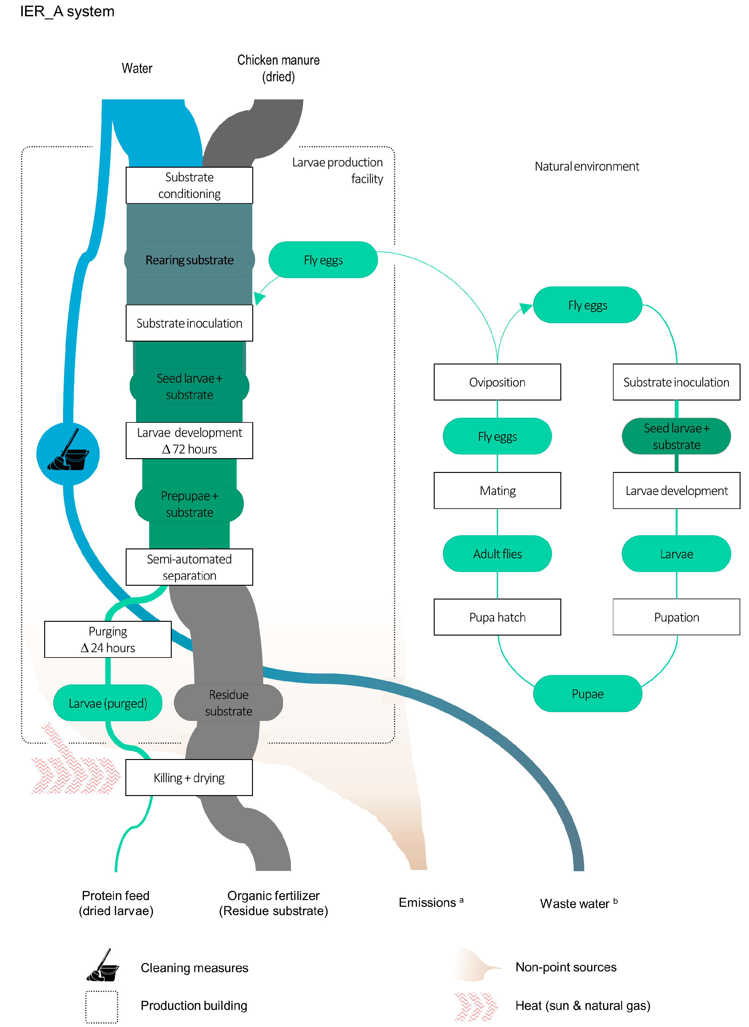Chicken manure, with 13.2 MJ per kg (DM), provided the lowest energy density of the substrate ingredients examined (Table 1). Due to a high dry matter (DM) content of about 90%, the conditioning of chicken manure required larger amounts of water to achieve optimal moisture levels. 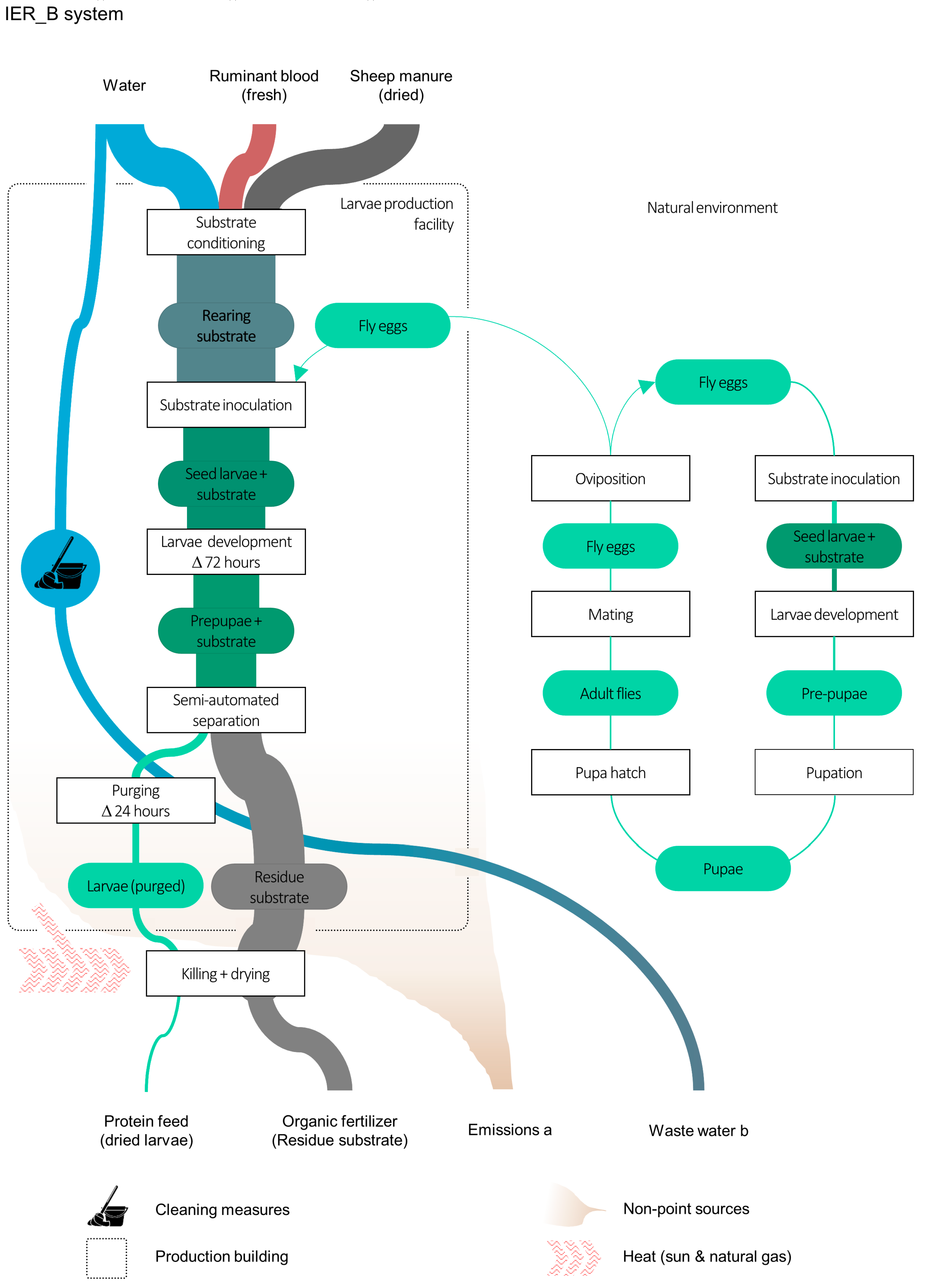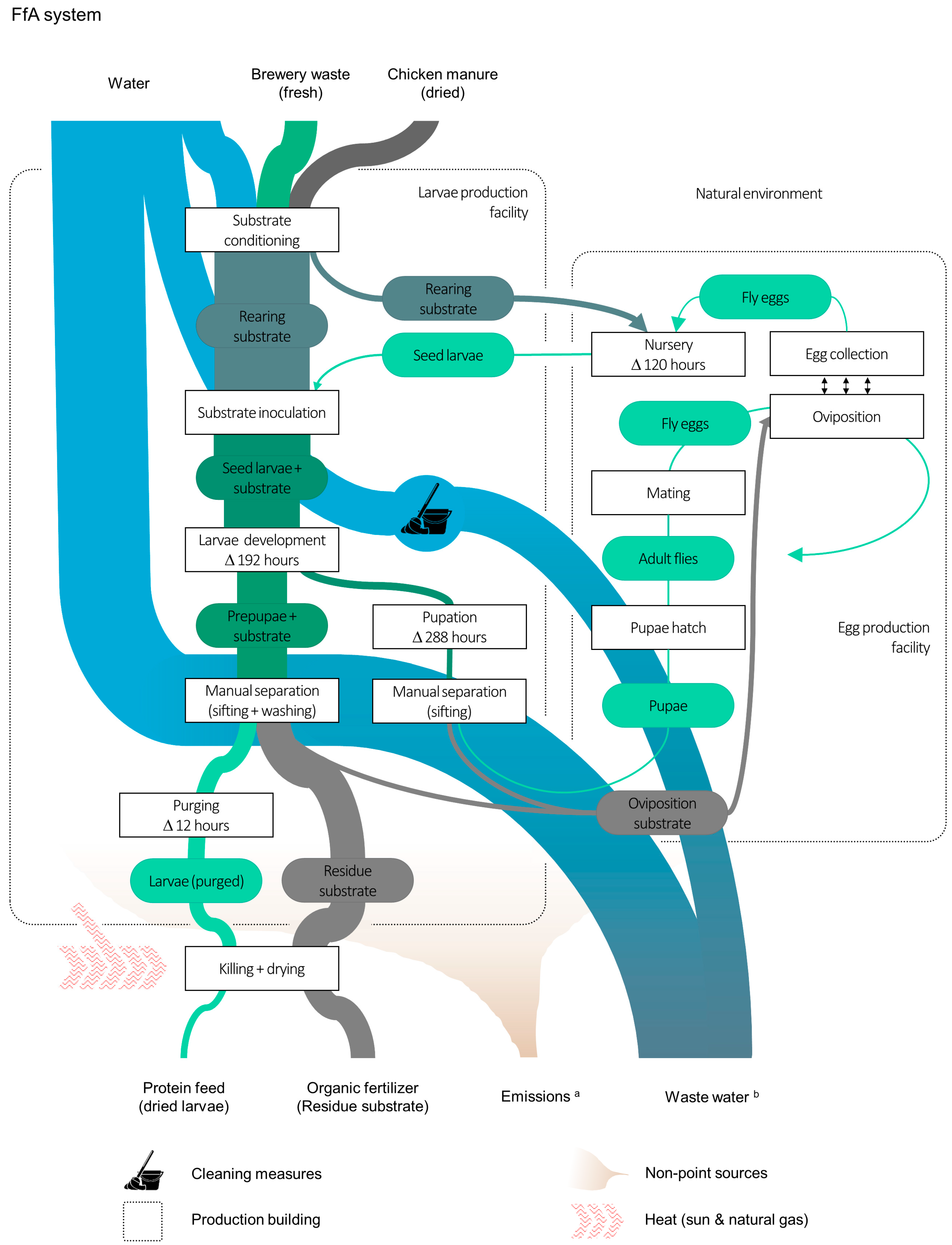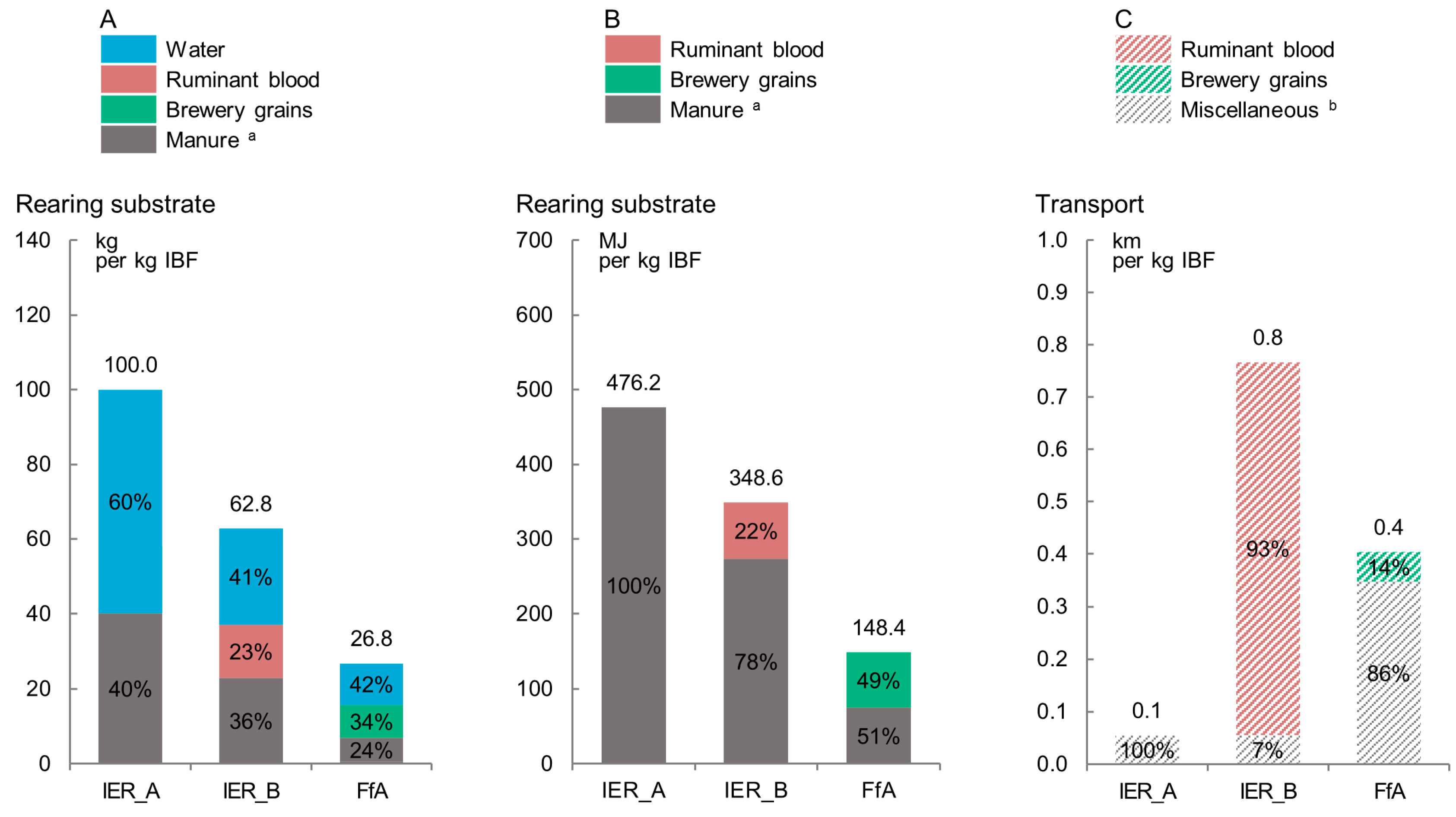The rearing substrate in the IER_A system (mixture of 40.0 kg chicken manure 59.9 L water) is calculated to have the lowest GEC of 4.8 MJ per kg fresh mass (FM) (Table 3). Correspondingly, the IER_A system is assessed with the lowest conversion efficiency (100.0 kg moistened rearing substrate/kg IBF) and the highest co-product output (28.0 kg residue substrate). The mixture of sheep manure, ruminant blood and water (IER_B system) arrives at a higher GEC (5.6 MJ/kg FM), which likewise coincides with a higher conversion efficiency (62.8 kg rearing substrate/kg IBF) and lower unit output of residue substrates (16.0 kg). The highest conversion efficiency and lowest residue substrate output amongst the IBF systems is calculated for the FfA system. To produce 1 kg dried H. illucens larvae and 7.1 kg residue substrate, the FfA system uses 26.8 kg substrate (mixture of dried chicken manure, fresh brewery waste and water) with a GEC of 5.5 MJ per kg FM (Table 3). The mass contribution of different substrate ingredients in each system can be retraced from Figure 1A.

Differences in the conversion efficiencies are not solely due to differing energy densities of the substrate ingredients. Less obvious, but equally important are nutritional properties, such as protein content, and biophysical factors (e.g., porosity and aeration of the rearing medium) that affect the ability of insect larvae to extract nutrients from the substrates provided. The relationship between conversion efficiency and the output of residue substrate becomes clearer when comparing the systems’ conversion efficiencies by measurement of calorie input (Figure 1B).

The IER_A system is the least efficient in terms of calorie utilisation, expending 476.2 MJ caloric energy to produce 1 kg IBF and 28 kg residue substrate. The IER_B and FfA systems follow with 348.6 MJ and 148.4 MJ per kg IBF, respectively (Figure 1B). The specific biophysical cause-effects underlying the differences between the IER systems cannot be clarified from the available data. It can be presumed, however, that advantages of the IER_B system result of the high protein content of ruminant blood [11,30]. The efficient calorie utilisation of the FfA system, on the other hand, is probably cause of two concurrent effects; favourable substrate characteristics (i.e., energy and protein content, porosity, water holding capacity, etc.) and a longer lasting growth phase (see Section 3.2).

Although the use of substrate combinations appears to benefit the conversion efficiency of the systems, it also comes at the cost of increased sourcing efforts, i.e., higher input of transportation and labour (Figure 1C). Although all three systems are assumed to be in close proximity to the manure producing sites, the use of more than one substrate is associated with additional transportation needs. Using only chicken manure from a poultry farm nearby, transportation in the IER_A system is limited to the sourcing of production and ancillary material, as well as the sale of process products (i.e., miscellaneous). Frequent trips using a motorbike to a generic market within 10 km proximity of the insect rearing facility constitutes a unit input of 0.1 km per kg IBF, which represents the lowest input of transportation of the three systems (Table 3 and Figure 1C). As the IER systems basically share the same process setup (see Section 2.1), there are no differences between the IER_A and IER_B system with regard to transportation for the sale of process products or collection of the chicken manure (Figure 1C; miscellaneous). The use of ruminant blood, however, requires sourcing from a slaughterhouse within 10 km proximity. Transport is facilitated by a commercial vehicle (3.5–7.5 t), with the blood transported in 40 L plastic barrels. As blood is highly perishable, it necessitates a steady procurement (every second day), which ultimately increases the unit input of transportation by 0.7 km per kg IBF and the input of labour (trained staff) by 0.1 h per kg IBF (Figure 1C and Table 3). The comparatively high transportation needs in the FfA system (0.4 km/kg IBF) are primarily due to a higher demand for nondurable auxiliary equipment (plastic trays, mosquito mesh, cleaning materials, etc.) and gas bottle exchange (Appendix D, Table A8). Sourcing of brewery waste by truck (7.5–16 t) from a brewery within 20 km proximity added 0.1 km per kg IBF, which represents about 14% of the total input of transportation (Table 3 and Figure 1C).

Whilst the process related gaseous emissions draw on generic emission data, the calculated emission patterns (relation between emitted substances) are the same in all three IBF systems, but are a function of the time that rearing substrates are exposed to open air (see also Section 2.1). With an output of 15.5 g CH₄, 0.3 g N₂O, 2.8 g NH₃ and 2.5 g volatile solids per kg IBF (emitted to air), the IER_A system is calculated to have the highest gaseous emissions. Despite conversion efficiency advantages, the FfA system gave the second highest emissions, due to the longer larval development time. The IER_B system gave the lowest gaseous emissions, with only about 64% the emissions of the IER_A system (Table 3).

3.2. Rearing Technique and Insect Species

Other factors influencing the conversion efficiency for insect larvae are the inoculation method used and the duration of the larval development phase [11,61]. Hermetia illucens has a longer life cycle, and consequently larval development phase, than M. domestica. The longer growth phase of H. illucens and the higher mass of individual larvae fosters the effective penetration and mixing of the rearing substrates and a greater degree of feeding resulting in a more efficient substrate conversion. Inoculation with larvae (i.e., artificial inoculation), improves the manageability of the process and mass flows, as stocking densities can be adjusted according to substrate quality and quantity [11,61].

Although an artificial substrate inoculation and longer larval development period appear to benefit the system’s conversion efficiency, this results in adverse effects on the input efficiency of space, labour and water (Figure 2).

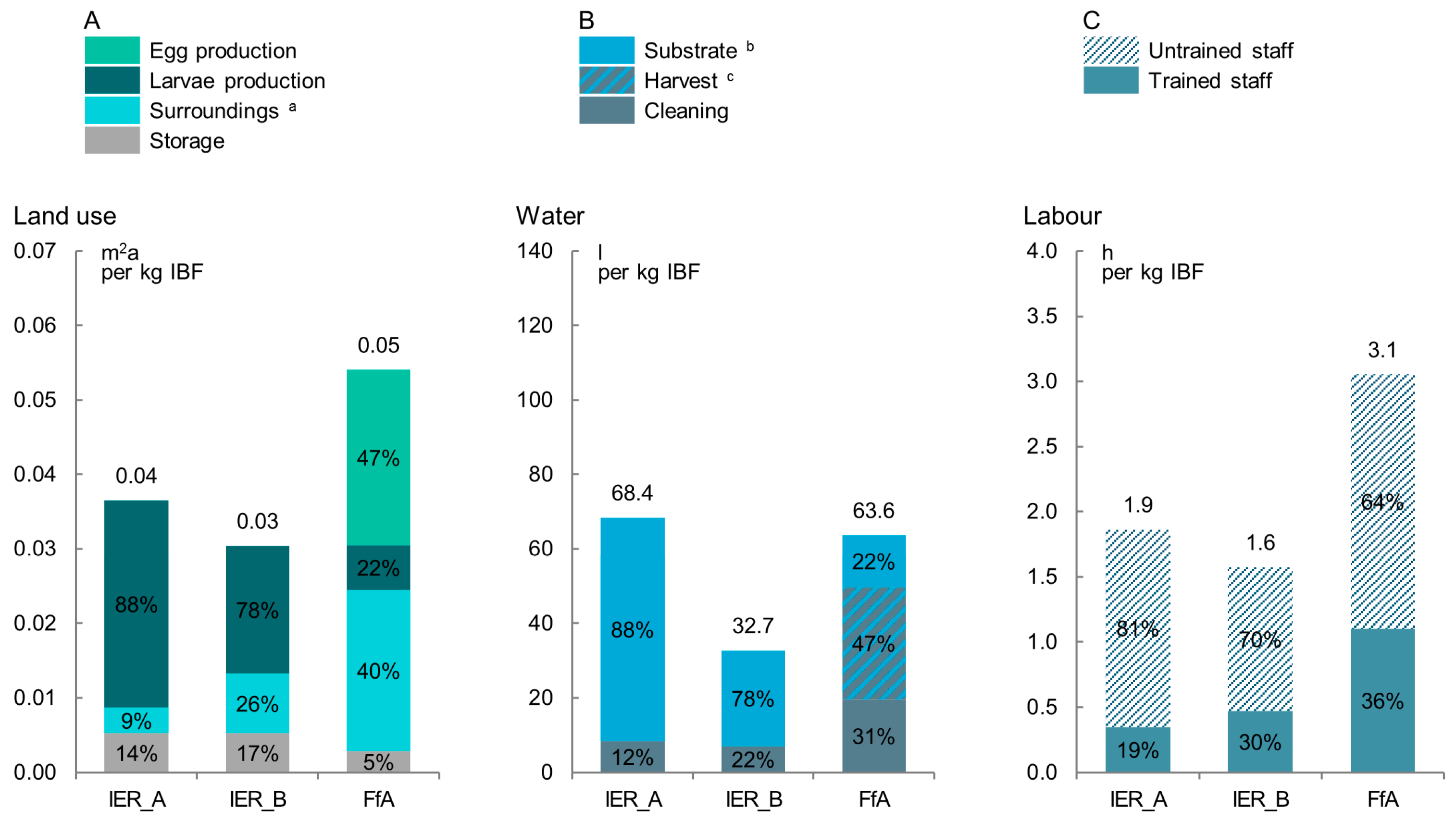
Disadvantages of artificial inoculation are particularly apparent in the relative input of land (Figure 2A). Like all land based animal production systems, the rearing of insect larvae involves the occupation of space over time. The unit input of land and built infrastructure are therefore a function of a system’s conversion efficiency, the species-specific life cycle and rearing technique. The effects of variable conversion efficiencies are best exemplified in the comparison of the IER_A and IER_B system (Figure 2A). Both systems share a similar production setup and advantages in conversion efficiencies translate directly into lower input of land. With 0.02 m²a per kg IBF (78% of total unit input) production of larvae in the IER_B system is more space efficient than larvae production in the IER_A system (0.03 m²a/kg IBF).

Favourable conversion efficiency and the use of artificial inoculation lower the relative input of land in the larvae production. With 0.01 m²a per kg IBF (22% of total land input), the rearing space in the FfA system is used most efficiently (Figure 2A). However, space use advantages in the larvae production unit are offset through additional space claims associated with the employed inoculation method and rearing of H. illucens adults for egg production. The maintenance of an egg production unit increases the space demand in the FfA system by 0.02 m²a per kg IBF (Figure 2A). Adding to this is a more intense use of the surrounding areas outside of the production facilities (0.02 m²a per kg IBF) for harvesting and drying of larvae, and for exposure to the sun of adult cages to promote mating and oviposition.

Further disadvantages of H. illucens and the artificial inoculation system arise from a more elaborate system design. The interplay between egg and larval production is organized through a sequence of complex operation steps that involve the use of additional production equipment, auxiliary materials, as well as consumables and supplies (Appendix A). Adding to this are materials and equipment necessary to prevent parasitoids attacking the H. illucens pupae before hatching [20]. The segmented process organisation and a larger number of tools and equipment not only increase the transportation needs (see Section 3.1), but also increase cleaning demands (Figure 2B). With 19.6 L water per kg IBF, the production in the FfA system is associated with the highest cleaning efforts. The IER_A and IER_B system follow with 7.1 and 8.4 L per kg IBF, respectively (Table 3). The breakdown of water input by activities further reveals that large amounts of water input in the FfA system are due to harvesting measures. To efficiently free the coarsely separated H. illucens larvae of substrate remnants, separated larvae are washed in water (see Section 2.1). The washing of larvae reduces the risk of a pathogen contamination of IBF, but eventually increases the water inputs in the FfA system to a total of 30.2 L per kg IBF (Figure 2B).

The more complex process organisation in the FfA system further translates into lower efficiency of labour inputs (Figure 2C). With a total of 3.1 h per kg IBF, the FfA system operates with the highest labour input of all the IBF systems. The operation of two interlinked production units requires additional monitoring and management needs resulting in relatively high employment of trained staff (l.2 h/kg IBF). 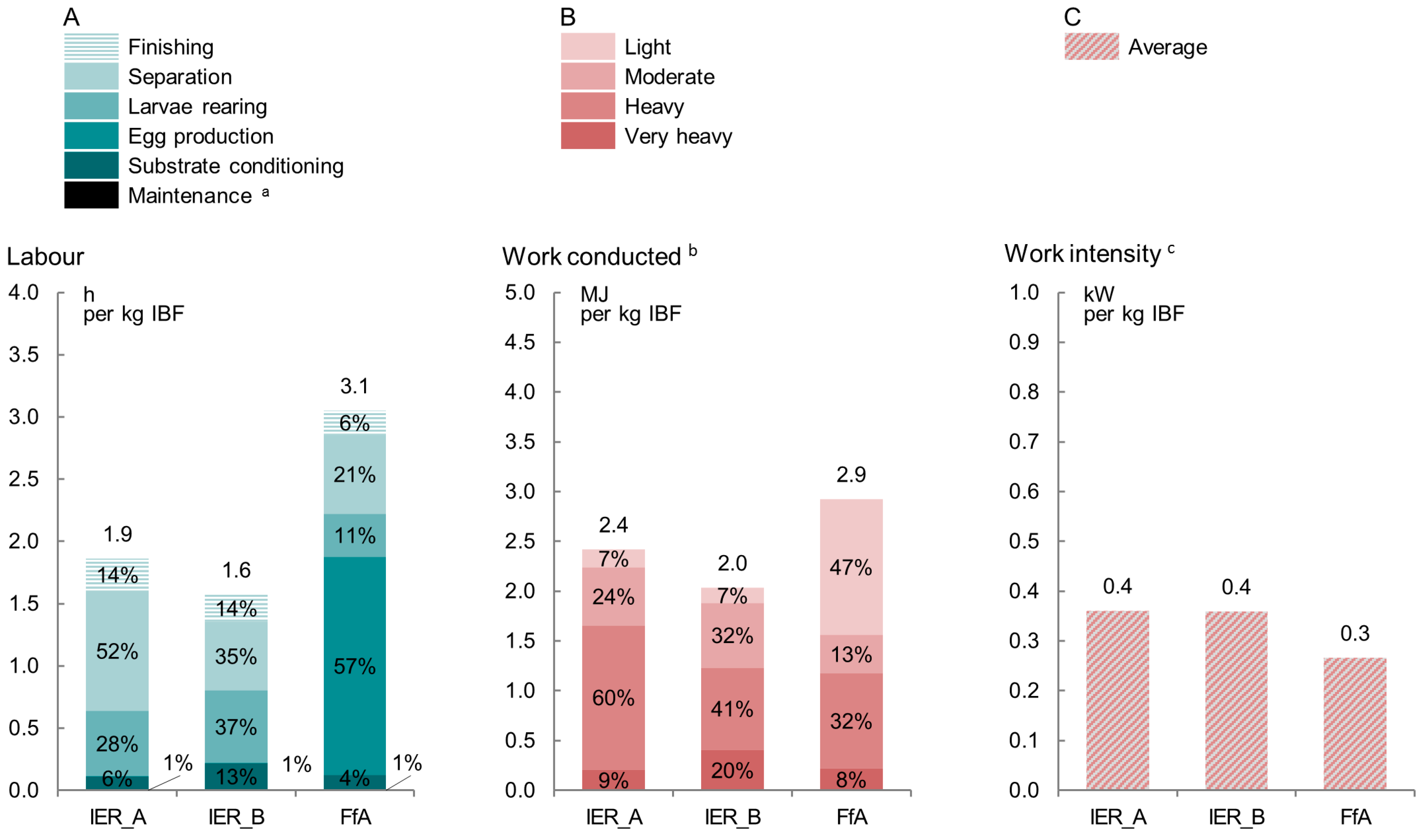The high labour input by untrained staff (1.9 h/kg IBF) is largely due to the more elaborate process organisation and longer process chain (see also Section 2.1). A breakdown of labour inputs by operational activities provides more detailed insights in Figure 3A.

In general, the IER systems operate with a lower unit input of labour (Figure 2C and Table 3). By using natural oviposition (omission of a separate egg production unit), unit inputs of labour in the IER_A and IER_B system are considerably lower than the FfA system (Figure 3A). The differences between the IER_A and IER_B system are due to differences in conversion efficiency. The higher unit output of residue substrate (28.0 kg/kg IBF) in the IER_A system increases the labour demand in the harvesting process (i.e., separation) up to 0.9 h per kg IBF (52% of total unit input). The IER_B system, on the other hand, shows higher labour demand in the substrate conditioning step (Figure 3A) as mixing of two substrate ingredients amounts to a unit input labour of 0.2 h per kg IBF (13% of total unit input).

The comparison of the IBF systems by work input (i.e., energy or physical human work conducted) is in line with prior observations, but arrives at more balanced results (Figure 3B). As labour inputs for egg production (1.8 h/kg IBF) are of “light work intensity” (0.7 MJ/h), the FfA system (2.6 MJ per kg IBF) shows comparable results to the IER_A (2.4 MJ/kg IBF) and the IER_B system (2.1 MJ/kg IBF). The differences in work input between the IER systems are due to the differing labour inputs in the separation step (heavy work intensity) and substrate conditioning step (very heavy work intensity). The IER_A system has the highest input of work with “heavy work intensity” (separation step), where a labour input of 1.0 h per kg IBF equals a work input of 1.4 MJ per kg IBF (60% of the total unit input). The IER_B system, on the other hand, has the highest share of work inputs of “very heavy work intensity” (substrate conditioning step), which accounts for about 20% (0.4 MJ per kg IBF) of the overall unit input of work (Figure 3B).

The differences between the IBF systems are less pronounced when labour inputs are characterised by average work intensity (input of energy consumed per hour). Despite the differing labour and work inputs, the IER systems involve similar work intensities (0.4 kW). The FfA system, ranking highest in unit input of labour and work, has the lowest work intensity (0.3 kW) (Figure 3C).

3.3. Climatic Conditions

The LCI results are also characterised by variation in climatic conditions, although this is a more indirect effect. While the warm and humid climate in tropical West Africa aids the rearing of the naturally occurring H. illucens, it causes increases in the unit input of fossil energy. Frequent precipitation and the high air humidity do not allow for sun drying of larvae. Instead, the drying of larvae was facilitated through a gas oven with 8 kWh power. To produce 1 kg of dried larvae (≤10% water) the gas oven burned natural gas with an energy equivalent of 3.3 MJ (Table 3). The IER systems, which only burn natural gas to support the killing of larvae in moments when exposure to sun is not possible (e.g., precipitation, cloud coverage), have a considerably lower unit input of fossil energy (0.7 MJ per kg IBF) (Table 3). However, it ought to be noted here that energy inputs in the killing and drying process are also subject to the specific surface/volume ratio of larvae. If larvae of both species would be killed and dried under the same conditions, advantages would still be given to M. domestica, as larvae are comparably smaller and of lower individual mass as the one of H. illucens.

Climatic conditions also influence the unit input of the production infrastructure. The service life of the machinery and construction materials (i.e., depreciation) is calculated as a function of the varying climatic conditions in the IER systems (semi-arid climate) and FfA system (tropic climate). Due to accelerated wear and tear in the humid conditions of tropical West Africa, the expected service life of production equipment in the FfA system was shorter than that for the IER systems (see also Appendix A). The effects are illustrated in the unit input of built infrastructure. With an expected service life of 15 years, the unit input of built infrastructure in the FfA system is about 3.3 times higher than the associated unit input of land (0.03 m²a) (Table 3). The built infrastructure in the IER systems is expected to last for 25 years, which results in lower unit inputs of 0.07 m²a (IER_A system) and 0.04 m²a (IER_B system) (Table 3).

3.4. Scale of Production

The differences in scale of production (i.e., daily IBF output) between the IBF systems are due to capacity constraints set in the modelling of the systems (see Section 2.2). The IER_A and IER_B system are modelled with a maximum daily output of 12 kg dried insect larvae (i.e., ≤10% water), which equates to production facilities with a surface area of 133.2 m² and 160.0 m², respectively (including storage facilities and surrounding outside areas). With the adult population restricted to the maintenance of 20,000 individuals (constant number), the FfA production system facilitates a maximum daily output of 9.6 kg dried insect larvae (i.e., IBF) and occupies a total surface area of about 189.0 m² (Table 3).

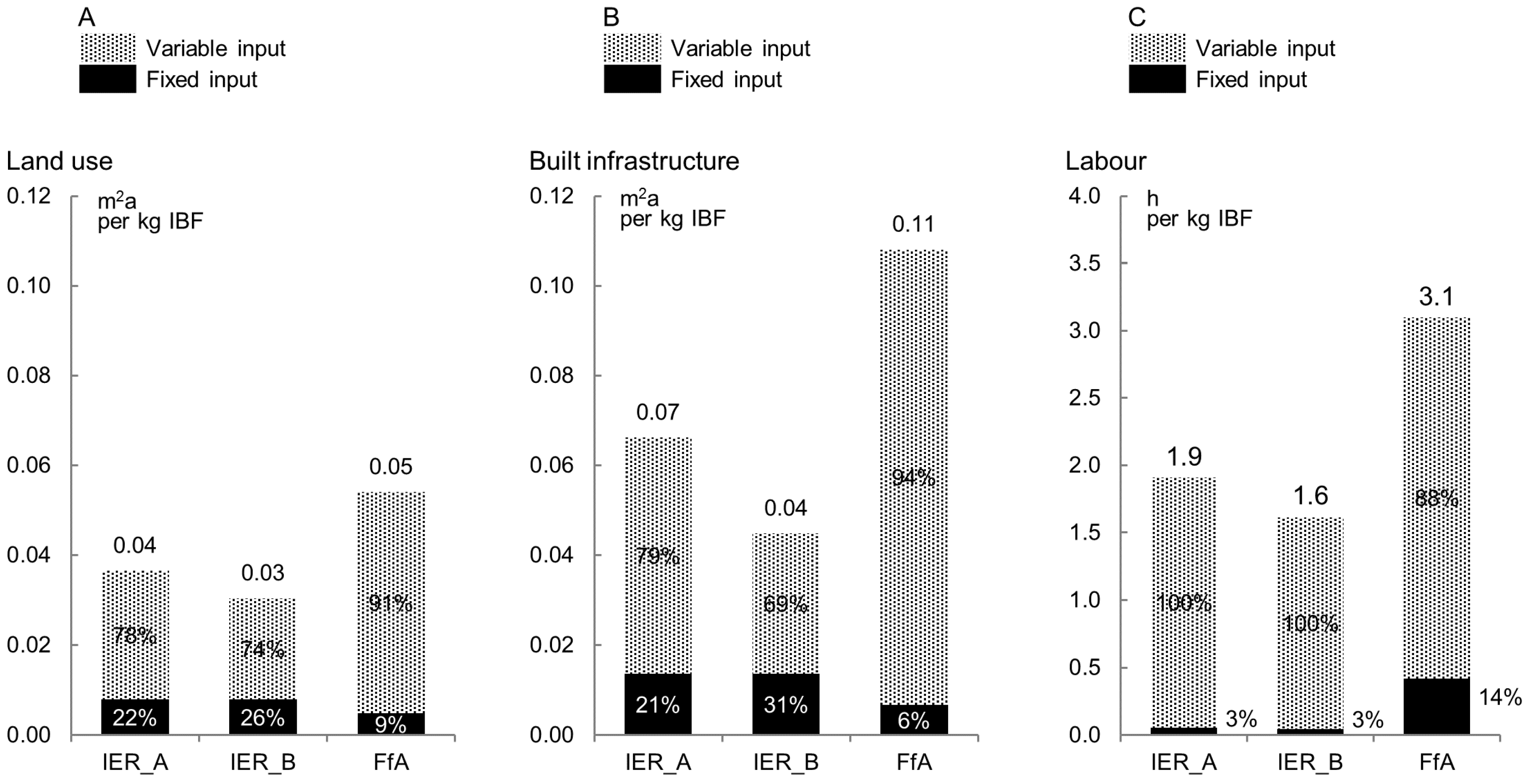
The effects of scale of production on the inventory results can be seen in the inputs of primary factors of production and their composition of scale dependent (variable) and scale independent (fixed, on short run) model parameters (Figure 4).

The generally low share of fixed inputs reflects the low level of automation and simplistic process setups of the IBF systems (Figure 4). The input of land (and built infrastructure) and labour are to a greater extent scale dependent, i.e., input changes are proportional to changes in output. The potential for efficiency gains through upscaling measures are therefore rather low. Economies of scale in the IER systems would primarily improve the input efficiencies of land and built infrastructure (Figure 4A,B). A further upscaling of the FfA system, on the other hand, would show notable effects in a relative decrease of unit labour inputs (Figure 4C).

Given the generally low conversion efficiencies, benefits of further upscaling would also depend on the availability of rearing substrates. Co-products, such as manure, blood and fresh brewery waste, are often already valorized in the form of fertilizers, food or feedstuff and thus an integrated part of agricultural value chains. Adding demand through IBF production would increase demand and prices of these co-products and in turn, may create shortages at other ends of the agricultural value chain (e.g., fertilizer, food or energy feeds). However, the output value of the co-product residue from IBF production, which is typically applied as a fertilizer to land, should also be considered. Whilst such reallocation effects seem feasible in the context of subsistence agriculture, it could potentially constrain a large-scale implementation of IBF in commercial operations.

4. Conclusions

The study has shown marked differences in the input efficiency of three modelled IBF systems. The most distinguishing factors are differences in conversion efficiencies (conversion of rearing substrate into IBF), which are mainly the result of a complex interaction of key determinants such as insect species, nutritional properties of the rearing substrate, rearing techniques and climatic conditions.

In general, substrate combinations with a high energy and protein content (e.g., fresh brewery waste and ruminant blood) enhanced the system’s conversion efficiency. The same applies to a longer growth phase of the larvae (promotes a greater degree of feeding) and use of artificial substrate inoculation (i.e., inoculation with nurtured larvae from a captive adult colony). However, as trade-offs exist between conversion efficiency and input efficiency of dependent input variables (e.g., space, built infrastructure, labour, water and transport), advantages in conversion efficiency lack comparability and permit no direct conclusions on the system’s overall performance.

The LCI analysis also showed that further upscaling would benefit the system’s input efficiencies. Though dependent on (and potentially constrained by) the availability of rearing substrates, a further upscaling would lower the unit input of labour, land and built infrastructure. However, to better leverage economy of scale effects, system designs should implement measures of automation and more specialised rearing equipment (e.g., improvement of harvesting techniques).

The study shows that a sustainable implementation of IBF production in West Africa requires further research and development. As input factors are strongly interrelated, statements on how to improve the system’s performances can currently only be made for each input factor individually (i.e., labour, water, space, etc.). To assess the application potential and examine conjectured sustainability advantages, it requires an environmental and economic characterization of the LCI models.

The simulation of up-scaled production versions required assumptions and approximations in both foreground and background inventory data. Given these multiple sources of model uncertainty, the predictive value of the presented analysis may vary according to the quality and extent of assumptions employed. Therefore, presented IBF systems have to be understood as hypothetical and derived findings and recommendations have to be interpreted and communicated with care. The presented datasets provide a basis for an environmental and economic life cycle assessment of IBF and shall serve as a reference point for scientific discussions and as an inspiration for future research in the domain of Eco-design and life cycle management.

References

1. Food & Agriculture Organization (FAO); International Fund for Agricultural Development (IFAD); World Food Programme (WFP). The State of Food Insecurity in the World: Meeting the 2015 International Hunger Targets: Taking Stock of Uneven Progress; Food & Agriculture Organization of the United Nations: Rome, Italy, 2015; ISBN 978-92-5-108785-5. [Google Scholar]
2. Haddad, L.; Hawkes, C.; Webb, P.; Thomas, S.; Beddington, J.; Waage, J.; Flynn, D. A new global research agenda for food. Nature 2016, 540, 30–32. [Google Scholar] [CrossRef] [PubMed]
3. United Nations Sustainable Development Knowledge Platform—SDGs. Available online: https://sustainabledevelopment.un.org/sdgs (accessed on 7 April 2017).
4. Marc, A.; Verjee, N.; Mogaka, S. The Challenge of Stability and Security in West Africa; World Bank Publications: Washington, DC, USA, 2015; ISBN 1464804656. [Google Scholar]
5. Hollinger, F.; Staatz, J.M. Agricultural Growth in West Africa Market and Policy Drivers; Food and Agriculture Organization of the United Nations (FAO): Rome, Italy, 2015. [Google Scholar]
6. Palazzo, A.; Rutting, L.; Zougmoré, R.; Vervoort, J.M.; Havlik, P.; Jalloh, A.; Aubee, E.; Helfgott, A.E.S.; Mason-D’Croz, D.; Islam, S. The Future of Food Security, Environments and Livelihoods in Western Africa: Four Socio-Economic Scenarios; CGIAR Research Program on Climate Change, Agriculture and Food Security (CCAFS): Copenhagen, Denmark, 2016. [Google Scholar]
7. Van Ittersum, M.K.; van Bussel, L.G.J.; Wolf, J.; Grassini, P.; van Wart, J.; Guilpart, N.; Claessens, L.; Groot, H.; Wiebe, K.; Mason-D’Croz, D.; et al. Can sub-Saharan Africa feed itself? Proc. Natl. Acad. Sci. USA Early Ed. 2016, 113, 14964–14969. [Google Scholar] [CrossRef] [PubMed]
8. Herrero, M.; Thornton, P.K. Livestock and global change: Emerging issues for sustainable food systems. Proc. Natl. Acad. Sci. USA 2013, 110, 20876–20881. [Google Scholar] [CrossRef] [PubMed]
9. Liu, J.; Mooney, H.; Hull, V.; Davis, S.J.; Gaskell, J.; Hertel, T.; Lubchenco, J.; Seto, K.C.; Gleick, P.; Kremen, C.; et al. Systems integration for global sustainability. Science 2015, 347. [Google Scholar] [CrossRef] [PubMed]
10. Maur, J.-C.; Shepherd, B. Connecting Food Staples and Input Markets in West Africa: A Regional Trade Agenda for ECOWAS Countries; World Bank: Washington, DC, USA, 2015. [Google Scholar]
11. Kenis, M.; Koné, N.; Chrysostome, C.A.A.M.; Devic, E.; Koko, G.K.D.; Clottey, V.A.; Nacambo, S.; Mensah, G.A. Insects used for animal feed in West Africa. Entomologia 2014, 2, 107–114. [Google Scholar] [CrossRef]
12. Adegoke, A.T.; Abioye, A.A. Improving livestock productivity: Assessment of feed resources and livestock management practices in Sudan-Savanna zones of West Africa. Afr. J. Agric. Res. 2016, 11, 422–440. [Google Scholar] [CrossRef]
13. United Nations. Harnessing Agricultural Potential for Growth and Development in West Africa; United Nations Economic Commission for Africa, Sub-Regional Office for West Africa: Niamey, Niger, 2012. [Google Scholar]
14. Jalloh, A.; Nelson, G.C.; Thomas, T.S.; Zougmoré, R.; Roy-Macauley, H. West African Agriculture and Climate Change: A Comprehensive Analysis; International Food Policy Research Institute (IFPRI): Washington, DC, USA, 2013; ISBN 9780896292048. [Google Scholar]
15. Zhou, Y.; Staatz, J. Projected demand and supply for various foods in West Africa: Implications for investments and food policy. Food Policy 2016, 61, 198–212. [Google Scholar] [CrossRef]
16. Organisation for Economic Co-operation and Development (OECD). Aquaculture in West Africa: A Sustainable Source of Food and Income? Organisation for Economic Co-operation and Development: Paris, France, 2006. [Google Scholar]
17. Kperegbeyi, J.I.; Meye, J.A.; Ogboi, E. Local chicken production: Strategy of household poultry development in coastal regions of Niger Delta, Nigeria. Afr. J. Gen. Agric. 2009, 5, 17–20. [Google Scholar]
18. Barroso, F.G.; de Haro, C.; Sánchez-Muros, M.J.; Venegas, E.; Martínez-Sánchez, A.; Pérez-Bañón, C. The potential of various insect species for use as food for fish. Aquaculture 2014, 422–423, 193–201. [Google Scholar] [CrossRef]
19. Bosch, G.; Vervoort, J.J.M.; Hendriks, W.H. In vitro digestibility and fermentability of selected insects for dog foods. Anim. Feed Sci. Technol. 2016, 221 Pt A, 174–184. [Google Scholar] [CrossRef]
20. Devic, E.; Leschen, W.; Murray, F.; Little, D.C. Growth performance, feed utilization and body composition of advanced nursing Nile tilapia (Oreochromis niloticus ) fed diets containing Black Soldier Fly (Hermetia illucens) larvae meal. Aquac. Nutr. 2017. [Google Scholar] [CrossRef]
21. Fanimo, A.O.; Susenbeth, A.; Südekum, K.H. Protein utilisation, lysine bioavailability and nutrient digestibility of shrimp meal in growing pigs. Anim. Feed Sci. Technol. 2006, 129, 196–209. [Google Scholar] [CrossRef]
22. Henry, M.; Gasco, L.; Piccolo, G.; Fountoulaki, E. Review on the use of insects in the diet of farmed fish: Past and future. Anim. Feed Sci. Technol. 2015, 203, 1–22. [Google Scholar] [CrossRef]
23. Van Huis, A.; Van Itterbeeck, J.; Klunder, H.; Mertens, E.; Halloran, A.; Muir, G.; Vantomme, P. Edible Insects: Future Prospects for Food and Feed Security; Food & Agriculrure Organisation of the United Nations (FAO): Rome, Italy, 2014; ISBN 9251075951. [Google Scholar]
24. Hwangbo, J.; Hong, E.C.; Jang, A.; Kang, H.K.; Oh, J.S.; Kim, B.W.; Park, B.S. Utilization of house fly-maggots, a feed supplement in the production of broiler chickens. J. Environ. Biol. 2009, 30, 609–614. [Google Scholar] [PubMed]
25. Kant, S.; Nautiyal, J.C. Sustainable joint forest management through bargaining: A bilateral monopoly gaming approach. For. Ecol. Manag. 1994, 65, 251–264. [Google Scholar] [CrossRef]
26. Makkar, H.P.S.; Ankers, P. Towards sustainable animal diets: A survey-based study. Anim. Feed Sci. Technol. 2014, 198, 309–322. [Google Scholar] [CrossRef]
27. Riddick, E.W. Chapter 16—Insect Protein as a Partial Replacement for Fishmeal in the Diets of Juvenile Fish and Crustaceans. In Mass Production of Beneficial Organisms; Morales-Ramos, J.A., Rojas, M.G., Shapiro-Ilan, D.I., Eds.; Academic Press: San Diego, CA, USA, 2014; pp. 565–582. ISBN 978-0-12-391453-8. [Google Scholar]
28. Sánchez-Muros, M.J.; Barroso, F.G.; de Haro, C. Chapter 10—Brief Summary of Insect Usage as an Industrial Animal Feed/Feed. In Insects as Sustainable Food Ingredients; Dossey, A.T., Morales-Ramos, J.A., Rojas, M.G., Eds.; Academic Press: San Diego, CA, USA, 2016; pp. 273–309. ISBN 978-0-12-802856-8. [Google Scholar]
29. Van Zanten, H.H.E.; Oonincx, D.G.A.B.; Mollenhorst, H.; Bikker, P.; Meerburg, B.G.; de Boer, I.J.M. Can the environmental impact of livestock feed be reduced by using waste-fed housefly larvae? In Proceedings of the 9th International Conference LCA of Food, San Francisco, CA, USA, 8–10 October 2014; pp. 8–10. [Google Scholar]
30. Koné, N.; Sylla, M.; Nacambo, S.; Kenis, M. Production of house fly larvae for animal feed through natural oviposition. J. Insects Food Feed 2017, 1–10. [Google Scholar] [CrossRef]
31. Pomalégni, S.C.B.; Gbemavo, D.S.J.C.; Kpadé, C.P.; Kenis, M.; Mensah, G.A. Traditional use of fly larvae by small poultry farmers in Benin. J. Insects Food Feed 2017, 1–6. [Google Scholar] [CrossRef]
32. Sánchez-Muros, M.J.; Barroso, F.G.; Manzano-Agugliaro, F. Insect meal as renewable source of food for animal feeding: A review. J. Clean. Prod. 2014, 65, 16–27. [Google Scholar] [CrossRef]
33. Halloran, A.; Roos, N.; Eilenberg, J.; Cerutti, A.; Bruun, S. Life cycle assessment of edible insects for food protein: A review. Agron. Sustain. Dev. 2016, 36, 1–13. [Google Scholar] [CrossRef]
34. Roffeis, M.; Muys, B.; Almeida, J.; Mathijs, E.; Achten, W.M.J.; Pastor, B.; Velásquez, Y.; Martinez-Sanchez, A.I.; Rojo, S. Pig manure treatment with housefly (Musca domestica) rearing—An environmental life cycle assessment. J. Insects Food Feed 2015, 1, 195–214. [Google Scholar] [CrossRef]
35. Smetana, S.; Palanisamy, M.; Mathys, A.; Heinz, V. Sustainability of insect use for feed and food: Life Cycle Assessment perspective. J. Clean. Prod. 2016, 137, 741–751. [Google Scholar] [CrossRef]
36. Salomone, R.; Saija, G.; Mondello, G.; Giannetto, A.; Fasulo, S.; Savastano, D. Environmental impact of food waste bioconversion by insects: Application of Life Cycle Assessment to process using Hermetia illucens. J. Clean. Prod. 2017, 140 Pt 2, 890–905. [Google Scholar] [CrossRef]
37. Prandini, A.; Paolo, D.P.; Francesca, T.; Giuliana, P.; Giovanni, P.; Paolo, B.; Antonella, D.Z.; Genciana, T.; Anna, D.-A.; Riccardo, F. Environmental impact of insect rearing for food and feed: State of the art and perspectives. Ital. J. Anim. Sci. 2015, 14, 132. [Google Scholar]
38. International Organization for Standardization (ISO). ISO 14040—Environmental Management—Life Cycle Assessment—Principles and Framework; ISO: Genève, Switzerland, 2006; Volume 14. [Google Scholar]
39. Institut National de la Statistiqu (INSTAT). 4ème Recensement Général de la Population et de l’Habitat du Mali—RGPH 2009 Résultats Provisoires; Institut National de la Statistiqu: Bamako, Mali, 2009. [Google Scholar]
40. Peel, M.C.; Finlayson, B.L.; McMahon, T.A. Updated world map of the Köppen-Geiger climate classification. Hydrol. Earth Syst. Sci. Discuss. 2007, 4, 439–473. [Google Scholar] [CrossRef]
41. United Nations Development Programme (UNDP). Human Development Report 2015; UNDP, Ed.; United Nations Development Programme: New York, NY, USA, 2015. [Google Scholar]
42. Nyantakyi-Frimpong, H.; Arku, G.; Inkoom, D.K.B. Urban agriculture and political ecology of health in municipal Ashaiman, Ghana. Geoforum 2016, 72, 38–48. [Google Scholar] [CrossRef]
43. GSS Ghana Statistical Service. Available online: http://www.statsghana.gov.gh/ (accessed on 5 March 2017).
44. Devic, E. Assessing Insect-Based Products as Feed Ingredients for Aquaculture; University of Stirling: Scotland, UK, 2016. [Google Scholar]
45. Devic, E.; Maquart, P.-O. Dirhinus giffardii (Hymenoptera: Chalcididae), parasitoid affecting Black Soldier Fly production systems in West Africa. Entomologia 2015, 3, 25–27. [Google Scholar] [CrossRef]
46. Weidema, B.P.; Bauer, C.; Hischier, R.; Mutel, C.; Nemecek, T.; Reinhard, J.; Vadenbo, C.O.; Wernet, G. The ecoinvent database 3.0. In Overview and Methodology Data Quality Guideline for the Ecoinventdatabase Version 3; Ecoinvent v2; Swiss Centre for Life Cycle Inventories: St. Gallen, Switzerland, 2013. [Google Scholar]
47. Association for Technology and Structures in Agriculture (KTBL). Emissionen der Tierhaltung. Grundlagen, Wirkungen, Minderungsmaßnahmen [Emissions from Animal Husbandry. Basic Principles, Effect Mechanisms, Mitigation Measures]; Association for Technology and Structures in Agriculture (KTBL): Darmstadt, Germany, 2002; ISBN 9783784321431. [Google Scholar]
48. Association for Technology and Structures in Agriculture (KTBL). Festmistaußenlagerung [External Storage of Solid Manure]; Association for Technology and Structures in Agriculture (KTBL): Darmstadt, Germany, 2011. [Google Scholar]
49. Association for Technology and Structures in Agriculture (KTBL). Betriebsplanung Landwirtschaft 2012/13 [Operational Planning Agriculture 2012/13]; Association for Technology and Structures in Agriculture (KTBL): Darmstadt, Germany, 2012; Volume 23, ISBN 978-3-941583-64-1. [Google Scholar]
50. Howley, E.T. Type of activity: Resistance, aerobic and leisure versus occupational physical activity. Med. Sci. Sports Exerc. 2001, 33, 364–369. [Google Scholar] [CrossRef]
51. Peregrina, C.A.; Lecomte, D.; Arlabosse, P.; Rudolph, V. Life Cycle Assessment (LCA) Applied to the Design of an Innovative Drying Process for Sewage Sludge. Process Saf. Environ. Prot. 2006, 84, 270–279. [Google Scholar] [CrossRef]
52. Aziz, N.A.; Wahab, D.A.; Ramli, R.; Azhari, C.H. Modelling and optimisation of upgradability in the design of multiple life cycle products: A critical review. J. Clean. Prod. 2016, 112, 282–290. [Google Scholar] [CrossRef]
53. Basbagill, J.; Flager, F.; Lepech, M.; Fischer, M. Application of life-cycle assessment to early stage building design for reduced embodied environmental impacts. Build. Environ. 2013, 60, 81–92. [Google Scholar] [CrossRef]
54. Eastwood, M.D.; Haapala, K.R. A unit process model based methodology to assist product sustainability assessment during design for manufacturing. J. Clean. Prod. 2015, 108, 54–64. [Google Scholar] [CrossRef]
55. Johnson, R.C.; Noguera, G. Accounting for intermediates: Production sharing and trade in value added. J. Int. Econ. 2012, 86, 224–236. [Google Scholar] [CrossRef]
56. Association for Technology and Structures in Agriculture (KTBL). Faustzahlen für die Landwirtschaft [Reference Figures in Agriculture]; Association for Technology and Structures in Agriculture (KTBL): Darmstadt, Germany, 2009; Volume 14, ISBN 978-3-939371-91-5. [Google Scholar]
57. Association for Technology and Structures in Agriculture (KTBL). Handhabung der TA Luft bei Tierhaltungsanlagen—Ein Wegweiser fuer die Praxis [Handling the TA Luft in Animal Husbandry—A Guide for the Practice]; Association for Technology and Structures in Agriculture (KTBL): Darmstadt, Germany, 2006; ISBN 978-3-939371-19-9. [Google Scholar]
58. CR Drying Chamber Heratherm, General Protoco—OGS400—Product Spezification. Available online: http://www.carlroth.com/catalogue/ (accessed on 14 March 2016).
59. Teravaninthorn, S. Transport Prices and Costs in Africa: A Review of the Main International Corridors/Supee Teravaninthorn, Gaël Raballand; Raballand, G., World, B., Eds.; World Bank: Washington, DC, USA, 2009; ISBN 9780821376508 0821376500. [Google Scholar]
60. Moore, J.C.; Berlow, E.L.; Coleman, D.C.; de Ruiter, P.C.; Dong, Q.; Hastings, A.; Johnson, N.C.; McCann, K.S.; Melville, K.; Morin, P.J.; et al. Detritus, trophic dynamics and biodiversity. Ecol. Lett. 2004, 7, 584–600. [Google Scholar] [CrossRef]
61. Čičková, H.; Kozanek, M.; Takac, P. Improvement of survival of the house fly (Musca domestica L.) larvae under mass-rearing conditions. Bull. Entomol. Res. 2013, 103, 119–125. [Google Scholar] [CrossRef] [PubMed]
62. Pawelzik, P.; Carus, M.; Hotchkiss, J.; Narayan, R.; Selke, S.; Wellisch, M.; Weiss, M.; Wicke, B.; Patel, M.K. Critical aspects in the life cycle assessment (LCA) of bio-based materials—Reviewing methodologies and deriving recommendations. Resour. Conserv. Recycl. 2013, 73, 211–228. [Google Scholar] [CrossRef]
63. Shibasaki, M.; Warburg, N.; Eyerer, P. Upscaling effect and Life Cycle Assessment. In Proceedings of the 13th CIRP International Conference of Life Cycle Engineering, Leuven, Belgium, 31 May–2 June 2006; pp. 61–64. [Google Scholar]
64. Gilgen, P.W.; Ackermann, R.; Fleischer, G. Stoff- und Energieflußanalyse für die 0.33l-Aluminium-Getraenkedose. In Produktionsintegrierter Umweltschutz; EF-Verlag für Energie- und Umwelttechnik: Berlin, Germany, 1994; pp. 467–474. [Google Scholar]
65. Ng, W.C.; You, S.; Ling, R.; Gin, K.Y.-H.; Dai, Y.; Wang, C.-H. Co-gasification of woody biomass and chicken manure: Syngas production, biochar reutilization, and cost-benefit analysis. Energy 2017, 139, 732–742. [Google Scholar] [CrossRef]
66. Ahmad, M.A.A. Production of Biogas From Poultry Manure. Bachelor Chem. Eng. 2015, 1, 1505–1510. [Google Scholar]
67. Barnett, G.M. Phosphorus forms in animal manure. Bioresour. Technol. 1994, 49, 139–147. [Google Scholar] [CrossRef]
68. Sorensen, P.; Jensen, E.S. Mineralization of carbon and nitrogen from fresh and anaerobically stored sheep manure in soils of different texture. Biol. Fertil. Soils 1995, 19, 29–35. [Google Scholar] [CrossRef]
69. Fasae, O.A.; Emiola, O.S.; Adu, I.F. Production of manure from West African Dwarf Sheep. Arch. Zootec. (España) 2009, 58 (Suppl. 1), 601–604. [Google Scholar]
70. Miller, S.F.; Miller, B.G. The occurrence of inorganic elements in various biofuels and its effect on ash chemistry and behavior and use in combustion products. Fuel Process. Technol. 2007, 88, 1155–1164. [Google Scholar] [CrossRef]
71. Heuzé, V.; Tran, G. Blood Meal—Tables of Chemical Composition and Nutritional Value—Feedipedia, a Programme by INRA, CIRAD, AFZ and FAO. Available online: https://www.feedipedia.org/node/221 (accessed on 9 September 2017).
72. Heuzé, V.; Tran, G.; Sauvant, D.; Lebas, F. Brewers Grains—Tables of Chemical Composition and Nutritional Value. Feedipedia, a Programme by INRA, CIRAD, AFZ and FAO. Available online: http://www.feedipedia.org/node/74 (accessed on 15 May 2017).
73. Reiling, B.A.; Extension Youth Livestock Specialis. Feed Dry Matter Conversions; University of Nebraska–Lincoln Extension, Institute of Agriculture and Natural Resources: Lincoln, NE, USA, 2011; pp. 1–4. [Google Scholar]
74. Shen, X.; Huang, G.; Yang, Z.; Han, L. Compositional characteristics and energy potential of Chinese animal manure by type and as a whole. Appl. Energy 2015, 160, 108–119. [Google Scholar] [CrossRef]
75. Bouchard, C.; Shephard, R.J.; Stephens, T. (Eds.) Physical Activity, Fitness, and Health: International Proceedings and Consensus Statement; Human Kinetics Publishers: Champaign, IL, USA, 1994. [Google Scholar]
76. Brown, J.R.; Crowden, G.P. Energy Expenditure Ranges and Muscular Work Grades. Occup. Environ. Med. 1963, 20, 277–283. [Google Scholar] [CrossRef]
77. Werner, F.; Scholz, R.M. Ambiguities in Decision-Oriented Life Cycle Inventories—The Role of Mental Models and Values, 1st ed.; Springer: Dordrecht, The Netherlands, 2005; ISBN 978-1-4020-3253-0. [Google Scholar]
Scheme 1. Schematic presentation of the unit processes and fundamental material and energy flows in the generic IER_A system, i.e., M. domestica reared on a substrate mixture of dried chicken manure and water (natural oviposition) in semi-arid West Africa. The width of arrows approximates flow quantities in the production process of the IER_A system. Associated numerical data on flow quantities are detailed in Section 3.1. a Process emission (non-point source), i.e., CH4, N2O, NH3, H2O and volatile solids (<10 μm). b Waste water from cleaning measures.
Sustainability 09 01697 sch001
Scheme 2. Schematic presentation of the unit processes and fundamental material and energy flows in the generic IER_B system, i.e., M. domestica reared on a substrate mixture of sheep manure, ruminant blood and water (natural oviposition) in semi-arid West Africa. The width of arrows approximates flow quantities in the production process of the IER_B system. Associated numerical data on flow quantities are detailed in Section 3.1. a Process emission (non-point source), i.e., CH4, N2O, NH3, H2O and volatile solids (< 10 μm). b Waste water from cleaning measures.
Sustainability 09 01697 sch002
Scheme 3. Schematic presentation of the unit processes and fundamental material and energy flows in the generic FfA system, i.e., H. illucens reared on a substrate mixture of fresh brewery waste, dried chicken manure and water (separate egg production unit) in tropical West Africa. The width of arrows approximates flow quantities in the production process of the FfA system. Associated numerical data on flow quantities are detailed in Section 3.1. a Process emission (non-point source), i.e., CH4, N2O, NH3, H2O and volatile solids (< 10 μm). b Waste water produced, e.g., due to cleaning measures, washing of larvae.
Sustainability 09 01697 sch003
Figure 1. Input efficiency of intermediate production factors in different insect based feed (IBF) production systems. Comparison of the IER_A, IER_B and FfA systems by: (A) mass input of substrate ingredients; (B) substrate specific calorie input; and (C) transport, associated with the provision of 1 kg IBF (≤10% water) to a generic market in West Africa. Contribution analysis of inventory items and activities illustrated as a proportion to the overall input. a Dried chicken manure (IER_A) and dried sheep manure (IER_B). b Provision and replacement of production and ancillary material, trade of IBF and residue substrate.
Sustainability 09 01697 g001
Figure 2. Input efficiency of intermediate production factors in different insect based feed (IBF) production systems. Comparison of the IER_A, IER_B and FfA system by: land use activities (A); causes of water consumption (B); and labour inputs of trained and untrained employees (C) associated with the provision of 1 kg IBF (≤10% water) to a generic market in West Africa. Contribution analysis of inventory items and activities illustrated as a proportion to the overall input. a Dried chicken manure (IER_A) and dried sheep manure (IER_B). b Conditioning of rearing substrates up to optimal moisture levels. c Water used in the separation and cleaning of H. illucens larvae (FfA system).
Sustainability 09 01697 g002
Figure 3. Characterization of labour input in different insect based feed (IBF) production systems. Characterization of labour inputs in the IER_A, IER_B and FfA system by contribution of operational activities (A); and breakdown of work inputs (energy) by: work intensity levels (B); and average work intensity (energy consumed per h) (C). Contribution analysis of operational activities and intensity levels are illustrated as a proportion to the overall unit input, associated with the provision of 1 kg IBF (≤10% water) to a generic market in West Africa. a Labour inputs relating to administrative tasks, maintenance and repair measures. b Work input (energy) calculated based on task-specific labour input and intensity levels (see Table 2). c Work intensity (i.e., power, or rate of work) calculated as energy consumed per unit time (h).
Sustainability 09 01697 g003
Figure 4. Input efficiency of primary production factors in different insect based feed (IBF) production systems. Comparison of the IER_A, IER_B and FfA system by unit inputs of: land (A); built infrastructure (B); and labour (C) associated with the provision of 1 kg IBF (≤10% water) to a generic market in West Africa. Contribution analysis of fixed and variable model parameters illustrated as a proportion to the overall input.
Sustainability 09 01697 g004